1. Electric fields yield chaos in microflows
Jonathan D. Posnera,b
, Carlos L. Pérezc
, and Juan G. Santiagod,1
a
Department of Mechanical Engineering, University of Washington, Seattle, WA 98195; b
Department of Chemical Engineering, University of Washington,
Seattle, WA 98195; c
Department of Mechanical Engineering, Arizona State University, Tempe, AZ 85287; and d
Department of Mechanical Engineering,
Stanford University, Stanford, CA 94305
Edited by* Parviz Moin, Stanford University, Stanford, CA, and approved July 30, 2012 (received for review April 23, 2012)
We present an investigation of chaotic dynamics of a low Reynolds
number electrokinetic flow. Electrokinetic flows arise due to cou-
plings of electric fields and electric double layers. In these flows,
applied (steady) electric fields can couple with ionic conductivity
gradients outside electric double layers to produce flow instabil-
ities. The threshold of these instabilities is controlled by an electric
Rayleigh number, Rae. As Rae increases monotonically, we show
here flow dynamics can transition from steady state to a time-
dependent periodic state and then to an aperiodic, chaotic state.
Interestingly, further monotonic increase of Rae shows a transition
back to a well-ordered state, followed by a second transition to a
chaotic state. Temporal power spectra and time-delay phase maps
of low dimensional attractors graphically depict the sequence
between periodic and chaotic states. To our knowledge, this is a
unique report of a low Reynolds number flow with such a sequence
of periodic-to-aperiodic transitions. Also unique is a report of
strange attractors triggered and sustained through electric fluid
body forces.
fluid mechanics ∣ electrohydrodynamics ∣ electrokinetic instability
Chaos in scalar fields driven by deterministic, low Reynolds
number (Re) flows was first described by H. Aref in the early
1980s (1); and chaotic advection was first leveraged to achieve
fast mixing in microchannel flows by Liu et al. (2). Indeed, deter-
ministic chaos has been studied in a wide variety of experimental
systems including turbulent flows (3), chemical reactions (4),
biological systems (4), and atomic force microscopy (5). Here,
we report evidence demonstrating the existence of dynamic
transitions from periodicity to aperiodicity and chaos in low Re
electrokinetic micron-scale flows. Microfluidic devices often use
liquid-phase electrokinetic phenomena to transport, concentrate,
and separate samples (6). Electrokinetics is the branch of elec-
trohydrodynamics that describes the coupling of ion transport,
liquid flow, and electric fields, and it is characterized by the
importance of electric double layers (7).
Typical electrokinetic flows, in order of 10 micron channels,
have low Reynolds numbers and are often stable as inertial forces
are strongly damped by viscous forces. However, applied electric
fields can couple with heterogeneous electric properties, in par-
ticular gradients of ionic conductivity, to generate electric body
forces in the bulk liquid (outside electric double layers). These
body forces can drive instability of bulk liquid flow fields. This
phenomena was first reported by Oddy et al. and termed electro-
kinetic instabilities (EKIs, see ref. 8). These electrokinetic flow
instabilities are driven by electric body forces, ρeE (where ρe is
the net free charge density and E is the electric field vector), in
these heterogeneous regions (8, 9). These body forces can be
distributed over relatively large flow regions and can exist outside
of electric double layers (10, 11).
In this paper, we present compelling evidence that an unstable,
low Reynolds number electrokinetic flow can become chaotic in
regimes characterized by the relative importance of electrical and
viscous forces. Temporal power spectra and time-delay phase-
maps distinguish between periodic and chaotic regimes. We be-
lieve this is the first demonstration of a strange attractor triggered
and sustained through electric fluid body forces in a low Reynolds
number flow. We show that the flow exhibits at least two periodic-
to-aperiodic (chaotic) transitions as the electric Rayleigh number
control parameter is monotonically increased. Although such
transitions are well known in the nonlinear dynamics field
(12–15) and occur in Taylor-Couette flows (16) (where fluid in-
ertia is important), we know of no reported microflow system with
such a sequence of transitions.
Results and Discussion
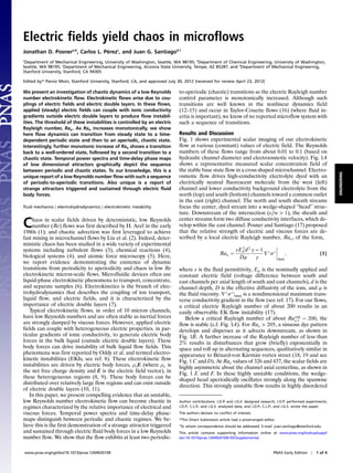
Fig. 1 shows experimental scalar imaging of our electrokinetic
flow at various (constant) values of electric field. The Reynolds
numbers of these flows range from about 0.01 to 0.1 (based on
hydraulic channel diameter and electroosmotic velocity). Fig. 1A
shows a representative measured scalar concentration field of
the stable base state flow in a cross shaped microchannel. Electro-
osmotic flow drives high-conductivity electrolyte dyed with an
electrically neutral fluorescent molecule from the west (left)
channel and lower conductivity background electrolyte from the
north (top) and south (bottom) channels toward a common outlet
in the east (right) channel. The north and south sheath streams
focus the center, dyed stream into a wedge-shaped “head” struc-
ture. Downstream of the intersection (x∕w > 1), the sheath and
center streams form two diffuse conductivity interfaces, which de-
velop within the east channel. Posner and Santiago (17) proposed
that the relative strength of electric and viscous forces are de-
scribed by a local electric Rayleigh number, Rae, of the form,
Rae ¼
εE2
a d2
Dμ
γ − 1
γ
∇Ã
σÃ

5. max
; [1]
where ε is the fluid permittivity, Ea is the nominally applied and
constant electric field (voltage difference between south and
east channels per axial length of south and east channels), d is the
channel depth, D is the effective diffusivity of the ions, and μ is
the fluid viscosity. ∇ÃσÃjmax is a nondimensional maximum trans-
verse conductivity gradient in the flow (see ref. 17). For our flows,
a critical electric Rayleigh number of about 200 results in an
easily observable EK flow instability (17).
Below a critical Rayleigh number of about Racrit
e;l ¼ 200, the
flow is stable (c.f. Fig. 1A). For Rae > 205, a sinuous dye pattern
develops and disperses as it advects downstream, as shown in
Fig. 1B. A further increase of the Rayleigh number of less than
2% results in disturbances that grow (briefly) exponentially in
space and roll up in alternating sequences, qualitatively similar in
appearance to Bénard-von Kàrmàn vortex street (18, 19 and see
Fig. 1 C and D). At Rae values of 326 and 437, the scalar fields are
highly asymmetric about the channel axial centerline, as shown in
Fig. 1 E and F. In these highly unstable conditions, the wedge-
shaped head aperiodically oscillates strongly along the spanwise
direction. This strongly unstable flow results in highly disordered
Author contributions: J.D.P. and J.G.S. designed research; J.D.P. performed experiments;
J.D.P., C.L.P., and J.G.S. analyzed data; and J.D.P., C.L.P., and J.G.S. wrote the paper.
The authors declare no conflict of interest.
*This Direct Submission article had a prearranged editor.
1
To whom correspondence should be addressed. E-mail: juan.santiago@stanford.edu.
This article contains supporting information online at www.pnas.org/lookup/suppl/
doi:10.1073/pnas.1204920109/-/DCSupplemental.
www.pnas.org/cgi/doi/10.1073/pnas.1204920109 PNAS Early Edition ∣ 1 of 4
ENGINEERING

6. scalar patterns and a well-mixed fluid a few channel widths down-
stream.
Fig. 2A shows a map of the temporal spectral intensity as a
function of the electric Rayleigh number (abscissa) and temporal
frequency (ordinate). Spectral density was calculated using a nor-
malized fluorescence intensity of the form,
I 0ðtÞ ¼
ðIðtÞ − hIitÞ
hIit
; [2]
where I 0ðtÞ is the fluorescence intensity taken at a point on the
channel centerline and x∕w ¼ 2 and the angle brackets and sub-
script t denote a temporal average. For Rae less than about 200,
the flow is stable and the power spectrum only shows power near
DC and low-amplitude image noise. Starting near Rae ¼ 205,
we observe periodic motion with at fundamental frequency of
f1 ¼ 42 Hz (at Rae ¼ 205) and weak harmonics at 2f1 and 3f1,
consistent with the periodic dye pattern of Fig. 1B. In the range
230 < Rae < 325, the frequency of the fundamental and harmo-
nic peaks slowly decrease, which coincides with an increase in
the disturbance wavelength, perhaps due to increasing electro-
osmotic flow (17). Subharmonic intensity peaks associated with
period doubling bifurcations are evident in the region near
Rae ¼ 290–350 (20). As an example, we labeled the subharmonic
peak at f1∕2, but we also observe peaks at 3f1∕4 and 5f1∕6. As
we discuss below, further increases in Rae result in a transition to
fully chaotic, aperiodic behavior. Such transitions from steady
state to time-dependent solutions, then period doubling, and
eventually fully chaotic behavior are well known in fluid flows.
However, it is most common for complexity in these flows to
increase monotonically with an increase of the controlling para-
A Rae = 100
B Rae = 210
C Rae = 214
D Rae = 223
E Rae = 326
-1
0
1
-1
0
1
-1
0
1
-1
0
1
x/w
F Rae = 437
-1
0
1
0 5 10
Fig. 1. Representative instantaneous scalar concentration fields of unstable
electrokinetic flows, each subject to constant electric field. The center-
to-sheath conductivity ratio γ is 100 and the electric Rayleigh number Rae is
indicated above each image. For our parameters, the conversion between
electric field and Rayleigh number is E ¼ 1.78Rae for electric field in V∕cm.
0 40 80 120 160 200
−8
−6
−4
log10
(PS)
Frequency [Hz]
0 40 80 120 160 200
−8
−6
−4
log10
(PS)
Frequency [Hz]
0 40 80 120 160 200
−8
−6
−4
log
10
(PS)
Frequency [Hz]
0 40 80 120 160 200
−8
−6
−4
log10
(PS)
Frequency [Hz]
0 40 80 120 160 200
−8
−6
−4
log
10
(PS)
Frequency [Hz]
Rae
Frequency(Hz)
200 250 300 350 400 450
0
50
100
150
regions of broad-band spectra
A
B Rae = 212
C
II III IV V
subharmonic peaks
I
D
E
F
Rae = 324
Rae = 362
Rae = 399
Rae = 449
Fig. 2. (A) Temporal power spectrum of I 0ðtÞ (in log10) as a function of
electric Rayleigh number and temporal frequency, f. Black and white colors
represent low and high spectral intensity, respectively. For Rae < 200, the
flow is stable (energy concentrated near f ¼ 0). Spectrum contains a funda-
mental frequency and harmonics for 205 < Rae < 325. Subharmonic peaks
appear at Rae ¼ 290–350. Aperiodic regimes are observed for Rae ranges
of 350–390 and 415–490 (labeled with horizontal bands above figure). Aper-
iodic regimes are defined here as those exhibiting a broadband power spec-
trum that is at least one order of magnitude above instrument noise. The
individual power spectra at five representative Rae are shown in (B–F) and
denoted with a roman numeral and vertical dashed line in (A). (B) Power
spectrum (in semilog coordinates) for Rae ¼ 212 shows flow instability with
a single-fundamental frequency at f ¼ 42 Hz and harmonics 2f and 3f. (C)
Spectrum for Rae ¼ 324 shows subharmonic peaks. (D) Aperiodicity with
broadband spectrum above instrumental noise (dashed line). (E) Second
time-periodic state with at least 11 observable harmonics. (F) Final chaotic
state.
2 of 4 ∣ www.pnas.org/cgi/doi/10.1073/pnas.1204920109 Posner et al.

7. meter. For example, increasing Rayleigh number, Ra, in Ray-
leigh-Bernard flows (13) results in transitions from steady flow
to time-dependent flow and, eventually, to fully chaotic, aperiodic
behavior.
The most interesting aspect of the current flow is the fact that,
unlike classic low-Reynolds fluid flows, the relation between
the controlling parameter, Rae, and dynamic complexity of the
system is not monotonic. As we increase Rae we observe steady
behavior (Rae < ∼200) and this is followed by time-periodic dy-
namics including a series of four harmonics (Rae ¼ 200 to 290),
evidence of period doubling (Rae ¼ 290 to 350), transition to a
chaotic state (350 to 390), a second time-periodic state with at
least 11 observable harmonics (390 to 415), and then a second,
final chaotic state (Rae > 415 to 490). That is to say, surprisingly,
the flow transitions sequentially in and out of chaos as Rae
increases so that, as the electric Rayleigh number is increased
from 200 to 490, we observe two sequential aperiodic regimes,
each of which is preceded by time-periodic regimes.
The two aperiodic regimes are labeled as solid horizontal
bands above Fig. 2A. The regimes at Rae ∼ 350–390 and Rae >
415 are strongly aperiodic as evidenced by well-distributed spec-
tral content (greater than 1 order of magnitude above noise,
as shown in Fig. 2 B–F). Other regions show some evidence of
aperiodicity, such as the region near Rae ∼ 320–340, which has
some broadband spectral content, but not as strongly as the latter
two regimes. Note that although the distinction between periodic
and aperiodic dynamics is typically made based on the existence
of broadband spectra, the minimum strength of broadband
spectra that warrants identification as aperiodicity is arbitrary.
Broadband spectra values significantly above 1 order of magni-
tude above instrument noise leaves us reasonably confident that
aperiodic dynamics exist. This definition is supported by the
phase maps presented below. The first and second aperiodic re-
gimes are also separated by a periodic region (Rae ∼ 390–415)
with a fundamental of f2 ¼ 15.8 Hz and harmonics at
2f2; 3f2…11f2 (see dashed line IVat Rae ¼ 399 in Fig. 2A). Per-
iodic windows sandwiched between aperiodic regimes have been
observed experimentally in, for example, the Belousov-Zabotins-
ky reaction (21) and in moderately high Reynolds number Taylor-
Couette flow (3, 16, 22). They are also well known as in mathe-
matical models with one-dimensional mappings such as the
Rössler attractor (4). To our knowledge, the current paper is the
first reported instance of a sequence of alternating periodic-
chaotic dynamical states in a low-Reynolds number flow system.
In this microflow, monotonic increase of the Rae controlling
parameter (proportional to electric field) drives the flow sequen-
tially into and out of chaos.
Example power spectra of the periodic and aperiodic regimes
are shown in Fig. 2 B–F for Rae ¼ 212, 324, 362, 399, and 449,
respectively. These Rae values are highlighted in Fig. 2A using
vertical dashed lines labeled I to V. At Rae ¼ 212, we see distinct
sharp peaks in the power spectra at the fundamental frequency
f1 ¼ 42 Hz and at harmonics 2f1, and 3f1. At Rae ¼ 324, we
observe clear evidence of period doubling and a broadening
of peaks as frequency increases. In the first chaotic region, at
Rae ¼ 362, we observe broadband spectral content tapering off
at higher frequencies and well above background noise. At
Rae ¼ 399, we observe the second periodic region, including a
series of over 11 harmonics. Lastly, at Rae ¼ 449, we observe the
second chaotic regime, which persists until the high-field limita-
tions of our experimental setup.
We constructed multidimensional phase-maps from time series
of normalized fluorescent intensity values, I 0ðtkÞ ðk ¼ 1…2;000Þ,
taken at x∕w ¼ 2 and y∕w ¼ 0 using the method of time delays
(23, 24). Here, time delay τ is used to construct a sequence of m-
dimensional points [I 0ðtkÞ; I 0ðtk þ τÞ; …I 0ðtk þ τðm − 1Þ] result-
ing in an m-dimensional phase-space trajectory. We employed the
method of Fraser and Swinney to obtain an optimum τ defined by
the first minimum of the mutual information function (25). Fig. 3
shows I 0ðt þ τÞ versus I 0ðτÞ phase-maps for Rae ¼ ðaÞ212, (b)
324, (c) 362, (d) 399, and (e) 449 for τ ¼ 2.6 ms. The sequence
−0.5 0 0.5
−0.5
0
0.5
I’(t+τ)
I. Ra
e
=212A
−0.5 0 0.5
−0.5
0
0.5
I’(t+τ)
II. Rae
=324B
−0.5 0 0.5
−0.5
0
0.5
I’(t+τ)
III. Rae
=362C
−0.5 0 0.5 1
−0.5
0
0.5
1
I’(t+τ)
IV.Rae
=399D
I’(t)
−0.5 0 0.5 1
−0.5
0
0.5
1
I’(t+τ)
I’(t)
V.Ra
e
=449E
Fig. 3. Phase-maps (I 0ðτÞ; I 0ðt þ τÞ) for Rae ¼ ðAÞ212, (B) 324, (C) 362, (D) 399,
and (E) 449. Together they illustrate the alternating sequence of periodic-
chaotic dynamical behavior that occurs as Rae is swept from 190 to 490.
The axis limits for D and E are expanded for clarity. The power spectra con-
tours (in the Rae vs. frequency plane) for each Rae number case shown here is
labeled with a roman numeral in Fig. 2A.
Posner et al. PNAS Early Edition ∣ 3 of 4
ENGINEERING

8. of attractors illustrates the sequence of periodic to aperiodic
dynamics transitions observed in the range of Rae of 150–490 with
each map showing between 50–120 orbits. For Rae ¼ 212
(Fig. 3A) the attractor shows an elliptical geometry (with a curve
thickness, which we attribute to experimental image noise) char-
acteristic of periodic dynamics. Well into the first periodic regime
and in the period doubling region, at Rae ¼ 324, the attractor
is multidimensional, as shown in Fig. 3C. Here, more complex
temporal evolution is characterized by weaving of smaller orbits
within larger ones. At Rae ¼ 362, we are within the aperiodic
power spectrum of the first chaotic regime (see Fig. 2 A and D),
and the respective attractor (cf. Fig. 3C) shows a dramatic change
including significant spreading of the orbits throughout the phase
map. Spreading of attractor orbits of chaotic flow has been
observed experimentally in the multiple periodic-to-chaotic re-
gime transitions in Taylor-Couette flows (3, 22). The phenomen-
on is also evident in classical dynamical systems attractors such as
the Rössler attractor and the differential-delay equation (Mack-
ey-Glass (4). Fig. 3D (Rae ¼ 399) shows the transition back to a
more ordered, periodic state as Rae is increased, and the attractor
shows a much tighter set of orbits. Fig. 3E shows the dynamical
structure for Rae ¼ 449 within the second aperiodic regime.
Here, the geometric structure found in previous attractors is lost,
suggesting higher attractor dimensionality and dynamics reminis-
cent of turbulence, but occurring here at Reynolds numbers less
than about 0.1.
The power spectra and phase-maps collectively are strong evi-
dence that the regions of aperiodicity are chaotic. Our data show
compellingly that that low Reynolds number EKI flows exhibit
alternating regimes of periodic motion and low dimensional
chaos. The transitions between periodic and aperiodic dynamics
occur twice (within Rae ranges of 350–390 and Rae > 415) as the
electric Rayleigh number is monotonically varied from 190 to
490. To our knowledge, this is the first report of such a sequence
of order-chaos transitions in low Reynolds number flows.
Materials and Methods
The experiments reported here were performed at the Stanford Microfluidics
Laboratory in Stanford University. We performed experiments in glass, cross-
shaped microchannels isotropically etched (D-shape) to w ¼ 50 μm wide
and 20 μm deep (Micralyne, Alberta, Canada). Direct current (DC) electrical
potentials and current were applied by submerging platinum wire electrodes
in the electrolyte solutions at end-channel reservoirs. We obtained instanta-
neous concentration fields of rhodamine B dye using epifluorescence micro-
scopy, high speed CCD camera imaging (Roper Scientific, Tucson, Arizona).
This dye is electrically net neutral (26) with a molecular weight of 479 g∕mol;
so our images are those of a passive, diffuse scalar and motion perpendicular
to material lines is due to advection of the bulk solvent (water) and not a drift
velocity due to the electric field. Potentials and CCD image acquisitions were
synchronized using a high voltage sequencer (LabSmith, Livermore, CA, USA).
Flows were imaged with a microscope (Nikon, Japan) equipped with a 20X,
NA ¼ 0.45 ELWD objective (Nikon, Japan). More details of the experimental
setup and conditions are given by Posner and Santiago (17) additional details
on the image acquisition and data analysis can be found in the SI Text.
ACKNOWLEDGMENTS. This work was supported by NSF PECASE (J.G.S. award
number CTS-0239080 and CAREER (J.D.P. award number CBET-0747917)
Awards.
1. Aref H (1984) Stirring by chaotic advection. J Fluid Mech 143:1–21.
2. Liu RH, et al. (2000) Passive mixing in a three-dimensional serpentine microchannel.
J Microelectromech Syst 2:190–197.
3. Brandstäter A, Swinney HL (1987) Strange attractors in weakly turbulent Couette-
Taylor flow. Phys Rev A 35:2207–2220.
4. Olsen LF, Degn H (1985) Chaos in biological systems. Q Rev Biophys 18:165–225.
5. Hu S, Raman A (2006) Chaos in atomic force microscopy. Phys Rev Lett 96:036107.
6. Squires TM, Quake SR (2005) Microfluidics: Fluid physics at the nanoliter scale. Rev
Mod Phys 77:977–1026.
7. Saville DA (1997) Electrohydrodynamics: The Taylor-Melcher leaky dielectric model.
Annu Rev Fluid Mech 29:27–64.
8. Oddy MH, Santiago JG, Mikkelsen JC (2001) Electrokinetic instability micromixing.
Anal Chem 73:5822–5832.
9. Lin H (2009) Electrokinetic instability in microchannel flows: A review. Mech Res Com-
mun 36:33–38.
10. Melcher JR, Taylor GI (1969) Electrohydrodynamics: A review of the role of interfacial
shear stresses. Annu Rev Fluid Mech 1:111–146.
11. Hoburg JF, Melcher JR (1979) Internal electrohydrodynamic instability and mixing of
fluids with orthogonal field and conductivity gradients. J Fluid Mech 73:333–351.
12. Feigenbaum MJ (1983) Universal behavior in nonlinear systems. Physica D 7:16–39.
13. Giglio M, Musazzi S, Perini U (1981) Transition to chaotic behavior via a reproducible
sequence of period-doubling bifurcations. Phys Rev Lett 47:243–246.
14. Lauterborn W, Cramer E (1981) Subharmonic route to chaos observed in acoustics. Phys
Rev Lett 47:1445–1448.
15. Simoyi RH, Wolf A, Swinney HL (1982) One-dimensional dynamics in a multicompo-
nent chemical reaction. Phys Rev Lett 49:245–248.
16. Buzug T, von Stamm J, Pfister G (1993) Characterization of period-doubling scenarios
in Taylor-Couette flow. Phys Rev E 47:1054–1065.
17. Posner JD, Santiago JG (2006) Convective instability of electrokinetic flows in a
cross-shaped microchannel. J Fluid Mech 555:1–42.
18. Bénard H (1908) Formation des centres de gyration à l’arrière d’un obstacle en
mouvement. C R Acad Sci Paris 147:839–842.
19. von Kármán T, Rubach H (1912) Über den mechanismus des flüssigkeits- und
luftwiderstandes. Phys Z 13:49–59.
20. Moon FC (1992) Chaotic and Fractal Dynamics (Wiley, New York).
21. Turner JS, Roux J-C, McCormick WD, Swinney HL (1981) Alternating periodic and
chaotic regimes in a chemical reaction—Experiment and theory. Phys Lett A 85:9–12.
22. Brandstäter A, et al. (1983) Low-dimensional chaos in a hydrodynamic system. Phys Rev
Lett 51:1442–1445.
23. Packard NH, Crutchfield JP, Farmer JD, Shaw RS (1980) Geometry from a time series.
Phys Rev Lett 45:712–716.
24. Takens F (1981) Dynamical Systems and Turbulence (Springer, Berlin).
25. Fraser AM, Swinney HL (1986) Independent coordinates for strange attractors from
mutual information. Phys Rev A 33:1134–1140.
26. Schrum KF, Lancaster JM, III, Johnston SE, Gilman SD (2000) Monitoring electro-
osmotic flow by periodic photobleaching of a dilute, neutral fluorphore. Anal Chem
72:4317–4312.
4 of 4 ∣ www.pnas.org/cgi/doi/10.1073/pnas.1204920109 Posner et al.

9. Supporting Information
Posner et al. 10.1073/pnas.1204920109
SI Text
Data Acquisition and Analysis. Summary of data acquisition and in-
stances of data rejection. We here summarize some features of
our scalar image data acquisition. Further details can be found
in ref. 1. The quantitative scalar field data we present in Figs. 2
and 3 are based on image sequences of 45 experiments compris-
ing 45 applied electric fields (nominal electric fields from 333 to
1122 V∕cm). These imaging experiments were strictly limited by
trade-offs between camera sensitivity, frame rate, region of inter-
est analyzed (subset of pixels used in CCD), and the amount of
data that fit in the RAM of our data acquisition computer. We
used a 16-bit, Peltier-cooled Photometrics CCD with on-chip gain
(Tucson, AZ). We chose a frame rate of 390 Hz. The data sets
each consisted of 1620 16-bit images with a CCD region of inter-
est of only 3 × 512 pixels (to reduce required memory and
increase data rate). One exception to this is the data of the lowest
electric field (a stable case) for which we obtained only about
1000 images (and extended these data to match the duration
of the other image series). The data of about half of the 12th
electric field and all of the 13th electric field (at E ¼ 455 and
466 V∕cm) were likely corrupted by severe background illumina-
tion (we attribute this to unshielded lighting from the room).
We therefore replaced the last approximately one-third of data
record 12 with a copy of its first approximate one-third, and re-
placed all of the data record 13 with the new data record 12. In all,
we replaced <3% of the data (about 1.3 of the 45 records) shown
in Fig. 2.
Further details of power spectrum analysis. We performed the KPSS
Test (2) to assess the stationarity of each of the experiments
shown in Fig. 2. We used the kpsstest function in Matlab (Math-
works) and used parameters recommended by Kwiatkowski et al
(2), including a 95% significance (alpha ¼ 0.05) level. In 40 of the
45 experiments, the test showed a failure to reject the null
hypothesis that the time series was trend stationary; suggesting
the data were trend stationary. Four of the remaining data sets
were spread apparently randomly in the low-electric field peri-
odic regimes (at the 3rd, 14th, 16th, and 25th lowest Rae cases
shown in Fig. 2). We attribute this to some slight fluctuation of
the illumination intensity supplied by our microscope’s mercury
bulb. The remaining, single data series, which was suggested by
the test to be nonstationary occurred within the first chaotic re-
gion in Fig. 2. However, the KPSS Test suggested the other six
experiments in this same chaotic region were stationary.
Prior to performing the power spectra, we removed slight lin-
ear trends. These linear trends are common in fluorescence quan-
titation of electrokinetic microflows and attributable to various
effects including variations in light intensity of the illumination
(in our case, the mercury bulb of the microscope), effects of elec-
trochemical reactions (at end channel reservoirs containing elec-
trodes) on the tracer dye, and/or photobleaching of the dye. The
typical linear trend in the data consisted of a variation of less than
about Æ3% of the measured mean value. The linear trend in 42 of
45 cases varied less than Æ7% and all varied less than Æ11%.
Prior to computing power spectra on the data, we used a
symmetric Hann window to minimize frequency leakage. Fig. 2
presents a map of 45 power spectra of the windowed time series
up to the Nyquist folding frequency of 195 Hz.
Lastly, the data shown in Fig. 2 used a virtual point detector
centered at x∕w ¼ 2. We integrated the intensity in a 3 × 3 region
in this subimage as a virtual point detector for our power spectra.
We also analyzed power spectra for temporal fluctuations of the
scalar at following additional downstream locations: x∕w ¼ 3.5,
5.3, and 7.1. These power spectra maps were qualitatively very
similar to those near x∕w ¼ 2, except for an expected attenuation
of the high frequency power due to the dispersion associated with
the combined effects of advection and molecular diffusion. This
similarity included the harmonics of the first (low electric field)
periodic regime, evidence of period doubling, the clear delination
of two chaotic regions, and the harmonics of the second (high
electric field) periodic regime.
1. Posner JD, Santiago JG (2006) Convective instability of electrokinetic flows in a cross-
shaped microchannel. J Fluid Mech 555:1–42.
2. Kwiatkowski D, Phillips PCB, Schmidt P, Shin Y (1992) Testing the null hypothesis of
stationarity against the alternative of a unit root. J Ecol 54:159–178.
Posner et al. www.pnas.org/cgi/doi/10.1073/pnas.1204920109 1 of 1