
Recommended
Recommended
More Related Content
Similar to Excel Practical - Exercise 4 Insert the following tab
Similar to Excel Practical - Exercise 4 Insert the following tab (13)
More from BetseyCalderon89
More from BetseyCalderon89 (20)
Recently uploaded
Recently uploaded (20)
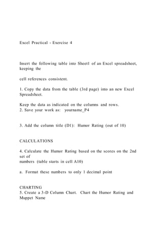
Excel Practical - Exercise 4 Insert the following tab
- 1. Excel Practical - Exercise 4 Insert the following table into Sheet1 of an Excel spreadsheet, keeping the cell references consistent. 1. Copy the data from the table (3rd page) into an new Excel Spreadsheet. Keep the data as indicated on the columns and rows. 2. Save your work as: yourname_P4 3. Add the column title (D1): Humor Rating (out of 10) CALCULATIONS 4. Calculate the Humor Rating based on the scores on the 2nd set of numbers (table starts in cell A10) a. Format these numbers to only 1 decimal point CHARTING 5. Create a 3-D Column Chart. Chart the Humor Rating and Muppet Name
- 2. a. Place the chart in a new worksheet title: Humor Rating b. Color the tab Blue c. Show the Muppets Names and Humor Rating on the chart a. Use data labels FORMATTING 6. Insert 2 rows at the top of the worksheet 7. Add the title (A1): The Muppets - Vital Statistics a. Center the title across the table b. Make it bold and underline it c. Chose the color and size font that is appropriate 8. Color each row with the color indicated in column C for each muppet. 9. Format the rest of the table to your liking. a. Choose appropriate fonts b. Choose appropriate border 10. Format the Humor Rating table to your liking a. Place borders around all of the cells b. Center the Scores 11. Bold the Column title in Row 3 and center them 12. Change the Tab Name and color to: Muppets and color it purple 13. Use Conditional Formatting to color the Humor Rating of 7.3 and higher to Bold White Font with a Dark Blue Background
- 3. 14. Fix the column widths so that you can see all of the data 15. Change the worksheets to Landscape orientation FINISHING TOUCHES 16. Insert a header in the center section. a. Type your name and <enter> b. Type the course ID (CGS1030) 17. Insert an image of the Muppets to the right of the table 18. Change the Document Properties a. Include your name b. Subject c. Tags (minimum of 3 – separate by commas) A B C D E F G H I J K 1 Muppet Name Creature Type Color
- 4. 2 Kermit Frog Green 3 Miss Piggy Swine Pink 4 Waldorf & Statler Grumpy Men Pink 5 Gonzo Unknown Blue/Gray 6 Animal Percussionist Red 7 Swedish Chef Swede Tan 8 Fozzie Bear Brown 9 10 Humor Rating 11 Score 1 Score 2 Score 3 Score 4 Score 5 Score 6 Score 7 Score 8 Score 9 Score 10 12 Kermit 6 5.8 6.3 8.122 8.3 7.55 7.6 8.5 7.1 6.6 13 Miss Piggy 4.3 5.6 3.8 7.53 8.4 6.8 4.9 8.1 9.1 7.7 14 Waldorf & Statler 4.9 4.9 9.2 8.4 7.5 9.64 8.3 4.5 9.64 9.62 15 Gonzo 8.2 5.7 5.79 7.5 8 7.2 9.4 5.9 8.32 8.4
- 5. 16 Animal 7.6 3.9 6.8 9.26 4.68 7.9 7.2 6.1 6.9 5.66 17 Swedish Chef 7.6 4.8 4.82 4.9 6.8 8.22 6.8 7.9 7.28 8.3 18 Fozzie 6.7 8.9 3.2 8.3 8.34 7.5 9.12 8.45 7.88 8.12 Week 6 Assignment Template In the land of free trade, the public does not view all industries as equal. Do you believe that is ethical? Do you believe that some industries are unfairly targeted? Should it be consumers’ choice to partake in products that are not healthy for them, or do those companies have an ethical obligation to protect people? In this assignment, you will choose one of the following industries to frame your paper: · The pharmaceutical industry. · The payday loan industry. · Cloning for medical purposes. Once you’ve gone through the worksheet and answered all the questions you will take that information and write your paper. It will basically be a transfer of information from the worksheet to a paper format. Do not just turn in the worksheet. It will be sent back for a
- 6. rewrite. 1. Choose an industry. 2. Will you be an advocate for the consumer or the industry? 3. Develop 3 reasons why you support the consumer or the industry. · Reason 1. · Supporting evidence for that reason. · Reason 2. · Supporting evidence for that reason. · Reason 3. · Supporting evidence for that reason. 4. Is it possible for a company to cater to both its best interest and that of the consumer simultaneously, or does one always have to prevail? · Reason 1. · Supporting evidence for that reason. · Reason 2. · Supporting evidence for that reason. · Reason 3. · Supporting evidence for that reason. Use at least two quality references. Note: Wikipedia and similar Websites do not qualify as academic resources. Your assignment must follow these formatting requirements: · This course requires use of Strayer Writing Standards (SWS). Please take a moment to review the SWS documentation for details. Introduction to Information Technology CGS1030 – Intro to IT Insert the following table into Sheet1 of an Excel spreadsheet,
- 7. keeping the cell references consistent. 1. Copy the data below into an Excel Spreadsheet. Keep the data as indicated on the columns and rows. 2. Save your work as yourname_P3 CALCULATIONS 3. Calculate the Total Score for the Home and Away Teams a. The Total Score is 4 points for each goal plus the Points b. These are for columns D and I 4. Enter the Row Title: TOTALS in cell A7 5. Calculate the following totals: a. Find the total goals and points b. These are for columns B, C, G and H ONLY FORMATTING 6. Insert 2 lines above the column titles 7. Title the worksheet as “British Football League Round 3 (Soccer)” a. Center the title across the table b. Use the font Algeria size 16 points 8. Center all of the column titles except for column A and F 9. Bold the column titles 10. Use conditional formatting for the TOTAL SCORE for the Home team.
- 8. a. Format the cells that show 20 points and greater to a BOLD white font with a Dark Blue Background i. NOTE: This is only for the specific column, not the entire table. 11. Name the worksheet tab RESULTS. 12. Color the tab Purple 13. Format the rest of the table to your liking a. Add borders around the cells b. Apply different colors, etc… 14. Insert an image appropriate to the data on the worksheet to the right of the table. A B C D E F G H I J 1 Home Team Goals Points Total Score Away Team Goals Points Total Score Winner 2 Liverpool 3 11 vs Wimbledon 4 14 3 Mansfield 2 6 vs Hayes 7 13 4 Stoneham 4 16 vs Sudbury 3 9 5 Darwen 1 11 vs Manchester 2 11 6 Blackpool 2 4 vs Bamsley 4 6
- 9. CHARTING 15. Graph the Home Team and their corresponding Total Score a. Use a 3d Column Cluster Chart b. Move the chart to a new sheet called Home Team c. Make sure you can see the data labels and make sure the title says TOTAL SCORE FINAL TOUCHES 16. Change the page orientation to landscape 17. Change the Document Properties i. Add your name ii. Add the subject iii. Add TAGS (Use a minimum of 3, separated by commas)