This project entails designing a distribution network while considering demand i.e. sales volume as the key demographic, along with population size. The key goal in this case is to design a network model that places distribution centers in the U.S. in such a manner so as to optimize flow for 3 given cases namely: A) 1 DC, B) 2 DC, and C) 3 DC

1. 1
Tableof Contents
OBJECTIVE:...................................................................................................................................... 2
PRODUCT DESCRIPTION:................................................................................................................ 2
METHODOLOGY:............................................................................................................................. 4
STEP 1: SELECTING POTENTIAL MARKETS / TARGET CITIES...............................................................4
STEP 2: CONVERTING THE GEOGRAPHIC COORDINATES INTO X AND Y COORDINATES .....................5
STEP 3: PLOTTING THE X AND Y COORDINATES ON A GRAPH...........................................................7
STEP 4: DEVELOPING THE CENTER OF GRAVITY (COG) MODEL: ........................................................7
STEP 5: DEFINING A NETWORK MODEL WITH 2 DISTRIBUTION CENTERS..........................................9
STEP 6: DEFINING A NETWORK MODEL WITH 3 DISTRIBUTION CENTERS........................................11
COST ANALYSIS:............................................................................................................................ 14
COST FOR 1 DISTRIBUTION CENTER: .............................................................................................14
COST FOR 2 DISTRIBUTION CENTERS:............................................................................................15
COST FOR 3 DISTRIBUTION CENTERS:............................................................................................17
CONCLUSIONS: ............................................................................................................................. 19
CONSIDERATIONS:........................................................................................................................ 19
GRAPHS......................................................................................................................................... 20
TableList
Table 1: Cities with key demographics and geographical locations…………………………………………….4
Table 2: Individual city data……………………………………………………………………………………………………….6
Table 3: Population dependence for quantities………………………………………………………………………...6
Table 4: Group distribution of cities for 2 DC network………………..........……………………………………..9
Table 5: Group distribution of cities for 3 DC network……………………………………………………………..11
Table 6: Cost calculations for 1 DC network…………………………………………………………………………….14
Table 7: Cost calculations for 2 DC network…………………………………………………………………………….15
Table 8: Cost calculations for 2 DC network…………………………………………………………………………….15
Table 9: Cost calculations for 3 DC network…………………………………………………………………………….17
Table 10: Cost calculations for 3 DC network…………………………………………………………………………..17
Table 11: Cost calculations for 3 DC network…………………………………………………………………………..18
FigureList
Figure1: ScrubEasy working prototype..............................................................................................3
Figure2: Selected cities plotted in the US map……………………………………………………….……………………5
Figure3: City map in x-y coordinates……………………………………………………………………………………………7
Figure 4: Selected cities plotted on the U.S. Map with 1st DC located………………………………………. 8
Figure 5: Selected cities plotted on the U.S. Map with 2 DCs located……………………………………….10
Figure 6: Selected cities plotted on the U.S. Map with 3 DCs located……………………………………….13

2. 2
OBJECTIVE:
This project entails designing a distribution network while considering demand i.e. sales volume
as the key demographic, along with population size. The key goal in this case is to design a
network model that places distribution centers in the U.S. in such a manner so as to optimize
flow for 3 given cases namely: A) 1 DC, B) 2 DC, and C) 3 DC
To design this model, we have used the COG (Center-Of-Gravity) model. For this model, the
following are the assumptions that we have based our network modeling on:
 We have selected 20 cities from across the USA from which 10 cities are from the top-20
cities in terms of population and the remaining 10 cities are from cities 21 to 100 in the
rankings
 We have assumed that there is 1 customer in each of these cities.
 The number of products sold per city is directly related to the respective city’s population
 Dividing cities into subgroups for 2 DC and 3 DC modeling, the division has been made
while taking into account the sales volume of the selected cities
 Apart from sales volume, population and distance are considered as secondary
demographics for further refinement
PRODUCT DESCRIPTION:
The product that the company is selling is ScrubEasy. ScrubEasy is a revolutionary scrub for
cleaning utensils. What segregates this scrub from all other scrubs in the market is its Texture
varying technology which allows it to alter its rigidity when brought in contact to cold and hot
water. For normal utensil cleaning, simply immerse the scrub in hot water and clean utensils
normally. For tough stains and/or debris such as rust on utensils,immerse the scrub in cold water.
This makes the scrub hard and thereby makes removing any kind of dirt, stains, rust, etc. from
utensils much simpler than any of its competition in the market.
The average cost that a household spends on scrubs per month is $3.92 per normal usage scrub
and $5.48 per heavy usage scrub.
Our company aims to launch the product at a competitive pricing of $6.99 per unit which is $2.41
per unit cheaper than the average $9.4 per 2 scrubs that an average household would spend on
scrubs.
The Go-to-market strategy of our product would therefore be organic marketing centered around
raising awareness about our product and how it simplifies the entire kitchen cleaning process.

3. 3
To illustrate this, the following is a picture showing the rigidity of the same scrub when immersed
in hot and cold water.
At first, the product may not seemas a significantvalue addition to a normal household, but upon
usage, customers would inevitably understand the value additions associated with the ScrubEasy
in comparison to any other scrubs in the market.
Kitchen application scrubs are inherently inexpensive, and have longer time deliveries simply
because they are not fragile, perishable, or prone to getting damaged or spoiled. The lot size per
consignment of scrubs is large and inventory holding costs are low when segregated for every
individual scrub that is stored at a warehouse. Also, since scrubs are a product that have a
continuous demand all-round the year, having a good inventory and safety stock is essential to
ensure higher customer service levels.
For the scope of this project, we are going to design a network to optimize the warehousing and
distribution of the ScrubEasy product across major cities of the U.S.
ScrubEasy
immersed in
hot water
ScrubEasy
immersed in
Cold water
Figure 1: ScrubEasy working prototype

4. 4
METHODOLOGY:
STEP 1: SELECTING POTENTIAL MARKETS / TARGET CITIES
In this step, we are going to choose cities that according to our research, are the ideal market
audience for our product. These cities have been selected by taking sales volume and population
as the key demographic (per 2010 census). Also, the respective latitude and longitude
coordinates of each of these states have been specified for further calculations as the project
progresses.
POPULATION SALES VOLUME LATITUDE LONGITUDE
NEW YORK 8.538 2,000,000 40.66 -73.93
LA 3.976 2,000,000 34 -118.4
CH 2.705 2,000,000 41.83 -87.68
HO 2.303 2,000,000 29.78 -95.39
PHEONIX 1.615 2,000,000 33.57 -112
PHILADELPHIA 1.568 2,000,000 40 -75.13
SAN ANTONIO 1.493 2,000,000 29.47 -98.52
SAN DIEGO 1.407 2,000,000 32.81 -117.13
DALLAS 1.308 2,000,000 32.79 -96.76
SAN JOSE 1.025 1000000 37.3 -121.81
BOSTON 0.673 1000000 42.33 -71.02
DETROIT 0.672 1000000 42.38 -83.1
ATLANTA 0.472 500000 33.76 -84.42
NASHVILLE 0.684 1000000 36.17 -86.78
ARLINGTON 0.392 500000 32.7 -97.12
DENVER 0.6 1000000 39.73 -104.99
MIAMI 0.453 500000 25.77 -80.2
PITTSBURGH 0.303 500000 40.43 -79.97
CINCINNATI 0.298 500000 39.14 -84.5
OKLAHOMA 0.638 1000000 35.46 -97.51
Table 1: Cities with key demographics and geographical locations
*population in million units

5. 5
When plotting the selected cities on the U.S. Map, the following is the result:
STEP 2: CONVERTING THE GEOGRAPHIC COORDINATES INTO X AND Y COORDINATES
For the scope of this project, we are implementing the center of gravity model (COG) due to
which the geographical coordinates of the cities cannot be used as an effective metric for
calculations. Therefore, the latitudes and longitudes of the cities need to be converted into their
respective x and y coordinates. To do this, we first select Houston as our point of origin i.e. (0.0)
simply because a majority of our selected cities are towards the east coast and mid-west which
makes San Diego an ideal point of origin for further calculations.
The new coordinates of the cities with San Diego as origin (0,0) is as follows:
Figure 2: Selected cities plotted on the U.S. Map

6. 6
CITIES POPULATION DEMAND LAT LONG Y-LAT X-LONG
NEW YORK 8.538 2,000,000 40.66 -73.93 7.85 43.2
LA 3.976 2,000,000 34 -118.4 1.19 -1.27
CH 2.705 2,000,000 41.83 -87.68 9.02 29.45
HO 2.303 2,000,000 29.78 -95.39 -3.03 21.74
PHEONIX 1.615 2,000,000 33.57 -112 0.76 5.13
PHILLI 1.568 2,000,000 40 -75.13 7.19 42
SAN
ANTONIO 1.493 2,000,000 29.47 -98.52 -3.34 18.61
SAN DIEGO 1.407 2,000,000 32.81 -117.13 0 0
DALLAS 1.308 2,000,000 32.79 -96.76 -0.02 20.37
SAN JOSE 0.945 1000000 37.3 -121.81 4.49 -4.68
BOSTON 0.673 1000000 42.33 -71.02 9.52 46.11
DETROIT 0.672 1000000 42.38 -83.1 9.57 34.03
ATLANTA 0.472 500000 33.76 -84.42 0.95 32.71
NASHVILLE 0.684 1000000 36.17 -86.78 3.36 30.35
ARLINGTON 0.392 500000 32.7 -97.12 -0.11 20.01
DENVER 0.6 1000000 39.73 -104.99 6.92 12.14
MIAMI 0.453 500000 25.77 -80.2 -7.04 36.93
PITTSBURGH 0.303 500000 40.43 -79.97 7.62 37.16
CINCINNATI 0.298 500000 39.14 -84.5 6.33 32.63
OKLAHOMA 0.638 1000000 35.46 -97.51 2.65 19.62
In table 1 and 2, the sales volume has been calculated by using the given data correlation
between population and demand i.e.
Population Range (1000s of people) # of Units Purchased Per Year (in 1000s)
0 to 500 500 units
500 to 1000 1000 units
>1000 2000 units
Table 3: Population dependence for quantities
Table 2: Individual city data

7. 7
STEP 3: PLOTTING THE X AND Y COORDINATES ON A GRAPH
STEP 4: DEVELOPING THE CENTER OF GRAVITY (COG) MODEL:
To develop the center of gravity model, the following is the equation that will be used to find the
x and y coordinates of the COG;
Where:
d – Total Demand
x, y – coordinates for individual customer
Solving for X and Y, we get:
X,Y coordinates with
reference to San Diego
21.726 3.01
Figure 3: City Map in x-y coordinates

8. 8
Then to find the actual location, we need to convert from reference to Houston to the original
one:
Latitude and Longitude
Coordinates for CG
35.814 -95.403
The latitude and longitude for CG i.e. 35.45 and 95.018 is located in Oklahoma. However, the
exact location is an agricultural field with minimal population. So, adjusting the CG location to
the nearest major city, we shortlisted Tulsa as our first Distribution Center (DC).
In figure 4, marks the 1st DC at Tulsa, Oklahoma. Tulsa’s population is 403,090.
This solves the first part of the project which is designing a distribution network centered around
a single Distribution center.
Figure 4: Selected cities plotted on the U.S. Map with 1st DC located

9. 9
STEP 5: DEFINING A NETWORK MODEL WITH 2 DISTRIBUTION CENTERS
In order to define a model with 2 distribution centers that will eventually serveallof the 20 stated
cities, we first need to divide the 20 cities into 2 groups based on geographical location as stated
in the question. The following is a table showing the two groups that the cities have been divided
into.
CITIES DEMAND X Y
LA 2000000 -1.27 1.19
HO 2000000 21.74 -3.03
PHEONIX 2000000 5.13 0.76
SA' 2000000 18.61 -3.34
SD 2000000 0 0
DALLAS 2000000 20.37 -0.02
SJ 1000000 -4.68 4.49
ARL 500000 20.01 -0.11
OC 1000000 19.62 2.65
DENVER 1000000 22.58 6.31
CITIES DEMAND X Y
BOSTON 1000000 46.11 9.52
DETROIY 1000000 34.03 9.57
ATL 500000 32.71 0.95
NASHVILLE 1000000 30.35 3.36
MIAMI 500000 36.93 -7.04
PITT 500000 37.16 7.62
CINN 500000 32.63 6.33
PHILL 2000000 42 7.19
NY 2000000 43.2 7.85
CHICAGO 2000000 29.45 9.02
Table 4: Group distribution of cities for 2 DC network

10. 10
For the first case, by applying the same calculations as in case 1, we will now find the location of
for the 1nd warehouse. The following are the resulting values:
X,Y coordinates with
reference to San Diego
11.39 0.29
Latitude and Longitude 33.101 -105.73
After mapping the latitude and longitude positions, the closest major city corresponding to the
calculated coordinates is Las Cruces, New Mexico. Memphis has a population of 101729 people
and a geographic location of 32.31°N, 106.76°W
Similarly, we will now apply the same calculations for the second group of cities so as to locate
the 2rd warehouse. The following are the resulting values:
X,Y coordinates with
reference to San Diego
6.772 37.227
Latitude and Longitude 39.58 -79.90
After mapping the latitude and longitude positions, the closest major city corresponding to the
calculated coordinates is Allentown, Pennsylvania. Allentown has a population of 120,443
people and a geographic location of 40.6°N, 75.49°W.
Figure 5: Selected cities plotted on the U.S. Map with 2 DCs located
Allentown, Pennsylvania DCLas Cruces, New Mexico DC

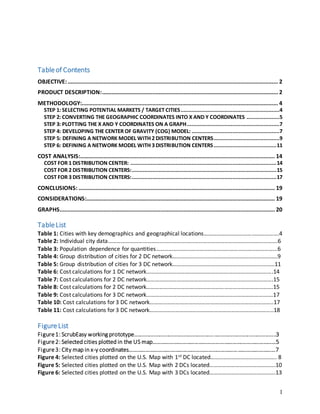
11. 11
STEP 6: DEFINING A NETWORK MODEL WITH 3 DISTRIBUTION CENTERS
In order to define a model with 3 distribution centers that willeventually serveallof the 20 stated
cities, we first need to divide the 20 cities into 3 groups based on sales volume as stated in the
question. The following is a table showing the three groups that the cities have been divided into.
WEST
CITY DEMAND X Y
L.A 2000000 -1.27 1.19
Phoenix 2000000 5.13 0.76
S.D 2000000 0 0
S.J 1000000 -4.68 4.49
Denver 1000000 22.58 6.31
Total Demand 8000000
SOUTH
CITY DEMAND X Y
Houston 2000000 21.74 -3.03
S.A 2000000 18.61 -3.34
Dallas 2000000 20.37 -0.02
Arlington 500000 20.01 -0.11
Miami 500000 36.93 -7.04
Oklahoma 1000000 19.62 2.65
Total Demand 8000000
EAST
CITY DEMAND X Y
New York 2000000 43.2 7.85
Chicago 2000000 29.45 9.02
Philadelphia 2000000 42 7.19
Boston 1000000 46.11 9.52
Detroit 1000000 34.03 9.57
Atlanta 500000 32.71 0.95
Nashville 1000000 30.35 3.36
Pittsburgh 500000 37.16 7.62
Cincinnati 500000 32.63 6.33
Total Demand 10500000
Table 5: Group distribution of cities for 3 DC network

12. 12
First, performing the calculations as done in STEP 5 for the Southern cities from table 5.1 in the
previous page, we get the following results:
X,Y coordinates with
reference to San Diego
21.191 -1.713
Latitude and Longitude 31.09 -95.938
After mapping the latitude and longitude positions, the closest major city corresponding to the
calculated coordinates is Houston, Texas. Houston has a population of 2.303 million people and
a geographic location of 29.76°N, 95.36°W
Second, performing the calculations as done in STEP 5 for the Western cities from table 5.2 in
the previous page, we get the following results:
X,Y coordinates with
reference to San Diego
3.20 1.875
Latitude and Longitude 34.64 -113.92
After mapping the latitude and longitude positions, the closest major city corresponding to the
calculated coordinates is Mesa, Arizona. Houston has a population of 484,587 people and a
geographic location of 33.41°N, 111.83°W.
Third, performing the calculations as done in STEP 5 for the Eastern cities from table 5.3 in the
previous page, we get the following results:
X,Y coordinates with
reference to San Diego
37.24 7.43
Latitude and Longitude 40.24 -79.88
After mapping the latitude and longitude positions, the closest major city corresponding to the
calculated coordinates is Allentown, Pennsylvania. Allentown has a population of 120,443
people and a geographic location of 40.6°N, 75.49°W.

13. 13
Figure 6: Selected cities plotted on the U.S. Map with 3 DCs located
Allentown, Pennsylvania DC
Mesa, Arizona DC

14. 14
COST ANALYSIS:
After calculating and locating the distribution centers for the 20 cities selected, the next step in
the process is to calculate the costs associated with transportation of the products from the
DCs to cities all across the country.
For this, the following are the assumptions that we have taken into account:
 Each individual shipment is of 1000 units load and fits completely in on truck
 The transportation cost per shipment from any DC to any city is $0.50 per mile
 The fixed costs per DC is $10,000,000 per year
 We ignore the additional variable costs like inventory holding costs, facility construction
costs, and start-up costs for simpler calculations
COST FOR 1 DISTRIBUTION CENTER:
DC-CITIES DISTANCE IN MILES PRODUCT SALES TRUCKS COST PER TRIP TOTAL COST
TULSA-NY 1351 2000000 2000 675.5 $1,351,000.00
TULSA-LA 1433.8 2000000 2000 716.9 $1,433,800.00
TULSA-CH 695.2 2000000 2000 347.6 $695,200.00
TULSA-HO 494.2 2000000 2000 247.1 $494,200.00
TULSA-PH 1065.2 2000000 2000 532.6 $1,065,200.00
TULSA-PHIL 1283.9 2000000 2000 641.95 $1,283,900.00
TULSA-SA 531.4 2000000 2000 265.7 $531,400.00
TULSA-SD 1418.2 2000000 2000 709.1 $1,418,200.00
TULSA-DA 257.4 2000000 2000 128.7 $257,400.00
TULSA-SJ 1690.4 2000000 2000 845.2 $1,690,400.00
TULSA-BO 1590.8 1000000 1000 795.4 $795,400.00
TULSA-DET 927.4 1000000 1000 463.7 $463,700.00
TULSA-ATL 784.1 500000 500 392.05 $196,025.00
TULSA-NASH 613.9 1000000 1000 306.95 $306,950.00
TULSA-ARL 275.6 500000 500 137.8 $68,900.00
TULSA-DENVER 693.6 1000000 1000 346.8 $346,800.00
TULSA-MIA 1445.4 500000 500 722.7 $361,350.00
TULSA-PITT 1000.1 500000 500 500.05 $250,025.00
TULSA-CINN 747.8 500000 500 373.9 $186,950.00
TULSA-OKH 106.1 1000000 1000 53.05 $53,050.00
$13,249,850.00
Table 5: Cost calculations for 1 DC network

15. 15
Total transportation costs for a one DC network in Tulsa, Oklahoma, is $12,963,575.
TOTAL COST= TOTAL TRANSPORTATION COST + FIXED COST PER DC
TOTAL COST= $13,249,850 + $10,000,000
TOTAL COST= $23,249,850
COST FOR 2 DISTRIBUTION CENTERS:
First, calculating the cost for the Las Cruces, New Mexico Distribution Center.
TOTAL COST= TOTAL TRANSPORTATION COST + FIXED COST PER DC
TOTAL COST= $5,289,025+ $10,000,000
TOTAL COST= $15,289,025
Second, calculating the cost for the second DC, i.e. Allentown, Pennsylvania.
DC-CITIES DISTANCE IN MILES PRODUCT SALES TRUCKS COST PER TRIP TOTAL COST
Las- LA 760.9 2000000 2000 380.45 $760,900.00
Las-HO 792.1 2000000 2000 396.05 $792,100.00
Las- Phoenix 389 2000000 2000 194.5 $389,000.00
Las- S.A 596.7 2000000 2000 298.35 $596,700.00
Las - S.D 683.2 2000000 2000 341.6 $683,200.00
Las - Dallas 680.6 2000000 2000 340.3 $680,600.00
Las - S.J 1099.8 1000000 1000 549.9 $549,900.00
Las - Arl 663.3 500000 500 331.65 $165,825.00
Las - OC 672 1000000 1000 336 $336,000.00
Las -Denver 669.6 1000000 1000 334.8 $334,800.00
$5,289,025.00
DC-CITIES
DISTANCE IN
MILES PRODUCT SALES TRUCKS COST PER TRIP TOTAL COST
Allentown - Boston 313.4 1000000 1000 156.7 $156,700.00
Allentown - Detroit 553.3 1000000 1000 276.65 $276,650.00
Allentown - Atl 792.5 500000 500 396.25 $198,125.00
Allentown -Nashville 796.5 1000000 1000 398.25 $398,250.00
Allentown - Miami 1245.9 500000 500 622.95 $311,475.00
Allentown - Pitt 281.7 500000 500 140.85 $70,425.00
Allentown - Cinci 549.5 500000 500 274.75 $137,375.00
Allentown - Phill 61.8 2000000 2000 30.9 $61,800.00
Allentown - NY 93.2 2000000 2000 46.6 $93,200.00
Allentown - Chicago 727.9 2000000 2000 363.95 $727,900.00
$2,431,900.00
Table 6: Cost calculations for 2 DC network
Table 7: Cost calculations for 2 DC network

16. 16
TOTAL COST= TOTAL TRANSPORTATION COST + FIXED COST PER DC
TOTAL COST= $2,431,900+ $10,000,000
TOTAL COST= $12,431,900
TOTAL COST FOR 2 DC NETWORK= $15,289,025 + $12,431,900= $27,720,925

17. 17
COST FOR 3 DISTRIBUTION CENTERS:
First, calculating the cost for the Houston, Texas Distribution Center.
DC-CITIES
DISTANCE IN
MILES
PRODUCT
SALES TRUCKS
COST PER
TRIP TOTAL COST
Houston - Houston 0 2000000 2000 0 $-
Houston - S.A 197.1 2000000 2000 98.55 $197,100.00
Houston - Dallas 239.1 2000000 2000 119.55 $239,100.00
Houston - Miami 1187.1 500000 500 593.55 $296,775.00
Houston - Okhlama 444.7 1000000 1000 222.35 $222,350.00
Houston - Arlington 255.6 500000 500 127.8 $63,900.00
$1,019,225.00
TOTAL COST= TOTAL TRANSPORTATION COST + FIXED COST PER DC
TOTAL COST= $1,019,225 + $10,000,000
TOTAL COST= $11,019,225
Second, calculating the cost for the Mesa, Arizona Distribution Center.
DC-CITIES
DISTANCE IN
MILES
PRODUCT
SALES TRUCKS
COST PER
TRIP TOTAL COST
MESA - L.A 388.4 2000000 2000 194.2 $388,400.00
MESA - PHEONIX 18.2 2000000 2000 9.1 $18,200.00
MESA - S.D 362.5 2000000 2000 181.25 $362,500.00
MESA - S.J 727.2 1000000 1000 363.6 $363,600.00
MESA - DENVER 851.2 1000000 1000 425.6 $425,600.00
$1,558,300.00
TOTAL COST= TOTAL TRANSPORTATION COST + FIXED COST PER DC
TOTAL COST= $1,558,300 + $10,000,000
TOTAL COST= $11,558,300
Table 8: Cost calculations for 3 DC network
Table 10: Cost calculations for 3 DC network

18. 18
Third, calculating the cost for the Allentown, Pennsylvania Distribution Center.
DC-CITIES
DISTANCE IN
MILES
PRODUCT
SALES TRUCKS
COST PER
TRIP TOTAL COST
Allentown - NY 93.2 2000000 2000 46.6 $93,200.00
Allentown -
CHICAGO 727.9 2000000 2000 363.95 $727,900.00
Allentown -
PHILADELPHIA 61.8 2000000 2000 30.9 $61,800.00
Allentown
BOSTON 313.4 1000000 1000 156.7 $156,700.00
Allentown -
DETRIOT 553.3 1000000 1000 276.65 $276,650.00
Allentown -
ATLANTA 792.5 500000 500 396.25 $198,125.00
Allentown -
NASHVILLE 796.5 1000000 1000 398.25 $398,250.00
Allentown -
PITTSBURGH 281.7 500000 500 140.85 $70,425.00
Allentown -
CINCINNATI 549.5 500000 500 274.75 $137,375.00
$2,120,425.00
TOTAL COST= TOTAL TRANSPORTATION COST + FIXED COST PER DC
TOTAL COST= $2,120,425+ $10,000,000
TOTAL COST= $12,120,425
TOTAL COST FOR 3 DCs= $11,019,225 + $11,558,300 + $12,120,425
TOTAL COST= $34,697,950
Table 11: Cost calculations for 3 DC network

19. 19
CONCLUSIONS:
The following are the total costs associated with different types of distribution networks as
calculated above.
Considering all the three models of distribution design, the most feasible option is the central
warehousing model for the company as it is the least capital intensive option.
However, while selecting an option, we need to consider other parameters as well apart from
only cost considerations.
Some of the factors that need to be considered alongside costs are:
 Customer satisfaction
 Service levels
 Lead times
 Inventory management
CONSIDERATIONS:
In a practical scenario, the following would be the governing factors and considerations to be
taken into account:
 Increasing the number of distribution centers would result in reducing lead times and
thus, improving customer satisfaction as the product will be more readily available to
the end consumer
 Increasing the number of distribution centers would reduce lead times and increase
product availability whilst increasing overall costs. Thus, a tradeoff between costs and
customer service levels would need to be done in order to select a model for
distribution network
 Furthermore, other pricing parameters such as labor costs, taxes, property costs, energy
costs, etc. need to be considered before setting up any distribution network
 A distribution network should be designed so as to adhere to requirements in terms of
demand variations, cross-docking, additional inventory storage, etc.
 Capability to handle reverse logistics as the distribution network becomes more
complex is essential to ensure a properly managed distribution network
MODEL COST
1 DISTRIBUTION CENTER $23,249,850
2 DISTRIBUTION CENTER $27,720,925
3 DISTRIBUTION CENTER $34,697,950

20. 20
GRAPHS
The succeeding pages show the costs associated for the different types of case scenarios that
we have considered for the scope of this project.
$1,351,000.00
$1,433,800.00
$695,200.00
$494,200.00
$1,065,200.00
$1,283,900.00
$531,400.00
$1,418,200.00
$2,574.00
$1,690,400.00
$795,400.00
$463,700.00
$196,025.00
$306,950.00
$68,900.00
$346,800.00
$361,350.00
$250,025.00
$186,950.00
$53,050.00
$- $200,000.00 $400,000.00 $600,000.00 $800,000.00 $1,000,000.00$1,200,000.00$1,400,000.00$1,600,000.00$1,800,000.00
TULSA-NY
TULSA-LA
TULSA-CH
TULSA-HO
TULSA-PH
TULSA-PHIL
TULSA-SA
TULSA-SD
TULSA-DA
TULSA-SJ
TULSA-BO
TULSA-DET
TULSA-ATL
TULSA-NASH
TULSA-ARL
TULSA-DENVER
TULSA-MIA
TULSA-PITT
TULSA-CINN
TULSA-OKH
TOTAL COSTFOR1 DISTRIBUTIONCENTER

21. 21
$760,900.00
$792,100.00
$389,000.00
$596,700.00
$683,200.00 $680,600.00
$549,900.00
$165,825.00
$336,000.00 $334,800.00
$-
$100,000.00
$200,000.00
$300,000.00
$400,000.00
$500,000.00
$600,000.00
$700,000.00
$800,000.00
$900,000.00
Las- LA Las-HO Las- Pheonix Las- S.A Las - S.D Las - Dallas Las - S.J Las - Arl Las - OC Las -Denver
TOTAL COSTFOR2 DISTRIBUTIONCENTERS (Las Crusis, New Mexico)
$156,700.00
$276,650.00
$198,125.00
$398,250.00
$311,475.00
$70,425.00
$137,375.00
$61,800.00
$93,200.00
$727,900.00
$-
$100,000.00
$200,000.00
$300,000.00
$400,000.00
$500,000.00
$600,000.00
$700,000.00
$800,000.00
Allentown -
Boston
Allentown -
Detriot
Allentown -
Atl
Allentown -
Nashville
Allentown -
Miami
Allentown -
Pitt
Allentown -
Cinci
Allentown -
Phill
Allentown -
NY
Allentown -
Chicago
TOTAL COSTFOR2 DISTRIBUTIONCENTERS (Allentown, Pennsylvania)

22. 22
$388,400.00
$18,200.00
$362,500.00 $363,600.00
$425,600.00
$-
$50,000.00
$100,000.00
$150,000.00
$200,000.00
$250,000.00
$300,000.00
$350,000.00
$400,000.00
$450,000.00
MESA - L.A MESA - PHEONIX MESA - S.D MESA - S.J MESA - DENVER
TOTAL COSTFOR3 DISTRIBUTIONCENTERS (Mesa, Arizona)
$-
$197,100.00
$239,100.00
$296,775.00
$222,350.00
$63,900.00
$-
$50,000.00
$100,000.00
$150,000.00
$200,000.00
$250,000.00
$300,000.00
$350,000.00
Houston - Houston Houston - S.A Hosuton - Dallas Houston - Miami Houston - Okhlama DC-CITIES
TOTAL COSTFOR3 DISTRIBUTIONCENTERS (Houston, Texas)

23. 23
$93,200.00
$727,900.00
$61,800.00
$156,700.00
$276,650.00
$198,125.00
$398,250.00
$70,425.00
$137,375.00
$-
$100,000.00
$200,000.00
$300,000.00
$400,000.00
$500,000.00
$600,000.00
$700,000.00
$800,000.00
Allentown -
NY
Allentown -
CHICAGO
Allentown -
PHILL
Allentown
BOSTON
Allentown -
DETRIOT
Allentown -
ATLANTA
Allentown -
NASHVILLE
Allentown -
PITTS
Allentown -
CINNICATTI
TOTAL COSTFOR3 DISTRIBUTIONCENTERS (Allentown, Pensylvania)