BOOTSTRAPPING TO EVALUATE RESPONSE MODELS: A SAS® MACRO
•
1 like•178 views

A handy SAS macro to produce validation metrics with corresponding confidence interval bands using bootstrapping sampling techniques.
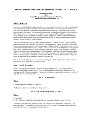
![P=1/(1+ exp(-Logit))
Whereas the Logit can take any value (-∞ ≤ Logit ≤ ∞), the probability (P) is constrained between 0 and 1.
MODEL EVALUATION
Once the model is built on a training sample, we conduct a non-biased assessment of model performance
by scoring the validation sample. In the Direct Marketing industry, gains tables (also called lift charts) are
commonly used to evaluate the effectiveness of the model in rank-ordering prospects. Scoring the
validation sample assigns the predicted probability of response to every individual. The scored data set is
then sorted in descending order by the score and binned into 10 or 20 equal-sized bands (ranks). The 10-
band approach creates equal sized deciles while the 20-band approach creates vigintiles.
The top band (Rank 1) holds prospects that are predicted as most likely to respond while the lowest scoring
prospects are found in the bottom band. Table 1 is an example of a gains table based on 17,964 individuals
in a validation sample.
Table 1
Decile # of
Prospects
Predicted
Probability of
Response
Actual
Response
Rate
Cum.
Response
Rate
Response
Lift
Cum.
Response
Lift
1 1,796 0.58014 0.44766 0.44766 199 199
2 1,796 0.49936 0.33352 0.39059 149 174
3 1,797 0.45296 0.30551 0.36222 136 161
4 1,796 0.41254 0.24388 0.33264 109 148
5 1,797 0.37403 0.21258 0.30862 95 137
6 1,796 0.33670 0.21771 0.29347 97 131
7 1,796 0.29625 0.16537 0.27517 74 123
8 1,797 0.25371 0.13856 0.25809 62 115
9 1,796 0.20685 0.10857 0.24148 48 108
10 1,797 0.14033 0.07234 0.22456 32 100
Total 17,964 0.35528 0.22456 0.22456 100 100
Column Descriptions:
Decile: The rank, based on splitting the sorted data into 10 bands.
# of Prospects : Total number of individuals per band. Each rank contains 10% of the file.
Predicted probability of response: On scoring, each individual is assigned a probability (p) of responding
based on the previously described formula. This column contains the mean value of p for the individuals in
the band. Rank 1 has a mean probability of response=0.58 while Rank 10 is 0.14.
Actual response rate: For each band, we count the number of individuals who actually responded to
the mailing (Response =1). Dividing this number by the total number of prospects in the band gives us the
actual response rate for that band. The response rate for Rank 1 is 44.8% while the response rate for the
overall sample is 22.5%.
Cum. response rate: For a given depth of file, we determine the number of actual number of
responders and divide this by the total depth of file. For example, the response rate for the top 2 bands
(20% of file, 3,592 prospects) is 39%.
Response Lift: Also called the response index, indicates how much better we are doing at each band
compared to the overall sample. The index is calculated as actual response rate at that band divided by the
overall response rate multiplied by 100. Rank 1 index is 199 [=0.44766/0.22456*100]. A response index of
199 indicates that individuals in Rank 1 had a 99% higher response rate compared to the overall rate. We
can also interpret it as 99% higher response rate than a no-model random mailing situation.
2](data:image/gif;base64,R0lGODlhAQABAIAAAAAAAP///yH5BAEAAAAALAAAAAABAAEAAAIBRAA7)
Recommended
Recommended
More Related Content
What's hot
What's hot (17)
Similar to BOOTSTRAPPING TO EVALUATE RESPONSE MODELS: A SAS® MACRO
Similar to BOOTSTRAPPING TO EVALUATE RESPONSE MODELS: A SAS® MACRO (20)
Recently uploaded
Recently uploaded (20)
BOOTSTRAPPING TO EVALUATE RESPONSE MODELS: A SAS® MACRO
- 1. BOOTSTRAPPING TO EVALUATE RESPONSE MODELS: A SAS® MACRO Anthony Kilili, Ph.D. 2006 Senior Manager, Credit Management & Modeling Bertelsmann Direct North America, Inc. BACKGROUND Response models in the direct marketing industry are constructed to rank-order a list of prospects based on their predicted propensity to respond to some mailing. In building the model, statisticians often use data from a previous campaign whereby a list of names was mailed to and their response tracked. For each prospect mailed, the response was either positive (responded, purchased etc) or negative (non-responders). The model is built on a binary response variable (yes or no) to predict the probability of response to a future campaign given a set of predictor attributes (inputs, independent variables). These attributes are a characterization of the prospect at the time of the mailing and may be in form of house-variables and/or appended external variables e.g. demographics. Although several methods exist to perform this modeling task (e.g. Neural networks, Genetic algorithms, Decision trees), the most commonly used approach is to build a Binary Logistic Regression (BLR) model. In doing so, the data are randomly split into training and validation samples. The training sample is used to generate the model while the validation sample is used to evaluate how the model performs when applied to new “unseen” data hence ensuring honest evaluation of the model. A good robust model will score with similar performance on both the training and validation datasets. A model that shows a very good ranking ability on the training data but works poorly on the validation sample is said to be an overfit model. This model has ‘learned’ specific patterns in the training data that are not present in the validation sample and would be expected to perform poorly if rolled out into production. This article provides a brief primer on some theoretical aspects of BLR and introduces a SAS macro that may be used as one of the tools for model evaluation. Binary Logistic Regression Binary Logistic Regression attempts to evaluate the relationship between a set of inputs (predictor, independent variables designated X1, X2, X3 etc.) to a binary response Y (typically labeled as Y=1 for responders and Y=0 for non-responders). The regression produces an equation that estimates the Logit of Y (log odds of response) which is defined as: Logit of Y = log(p/(1-p)) Where: P is the probability of response i.e. Prob(Y=1) The Logit is modeled as a linear function of n predictors as: Logit of Y= bo + b1X1 + b2X2 + b3X3 +…..+bnXn Where: bo = intercept b1---bn = Maximum Likelihood regression coefficients associated with input variables X1…Xn. The ultimate goal of building predictive models is to score new cases or prospects. The Logit of Y can easily be obtained by plugging the values of the inputs X1, X2…Xn into the equation and converted into probability of response by applying the logistic function: 1
- 2. P=1/(1+ exp(-Logit)) Whereas the Logit can take any value (-∞ ≤ Logit ≤ ∞), the probability (P) is constrained between 0 and 1. MODEL EVALUATION Once the model is built on a training sample, we conduct a non-biased assessment of model performance by scoring the validation sample. In the Direct Marketing industry, gains tables (also called lift charts) are commonly used to evaluate the effectiveness of the model in rank-ordering prospects. Scoring the validation sample assigns the predicted probability of response to every individual. The scored data set is then sorted in descending order by the score and binned into 10 or 20 equal-sized bands (ranks). The 10- band approach creates equal sized deciles while the 20-band approach creates vigintiles. The top band (Rank 1) holds prospects that are predicted as most likely to respond while the lowest scoring prospects are found in the bottom band. Table 1 is an example of a gains table based on 17,964 individuals in a validation sample. Table 1 Decile # of Prospects Predicted Probability of Response Actual Response Rate Cum. Response Rate Response Lift Cum. Response Lift 1 1,796 0.58014 0.44766 0.44766 199 199 2 1,796 0.49936 0.33352 0.39059 149 174 3 1,797 0.45296 0.30551 0.36222 136 161 4 1,796 0.41254 0.24388 0.33264 109 148 5 1,797 0.37403 0.21258 0.30862 95 137 6 1,796 0.33670 0.21771 0.29347 97 131 7 1,796 0.29625 0.16537 0.27517 74 123 8 1,797 0.25371 0.13856 0.25809 62 115 9 1,796 0.20685 0.10857 0.24148 48 108 10 1,797 0.14033 0.07234 0.22456 32 100 Total 17,964 0.35528 0.22456 0.22456 100 100 Column Descriptions: Decile: The rank, based on splitting the sorted data into 10 bands. # of Prospects : Total number of individuals per band. Each rank contains 10% of the file. Predicted probability of response: On scoring, each individual is assigned a probability (p) of responding based on the previously described formula. This column contains the mean value of p for the individuals in the band. Rank 1 has a mean probability of response=0.58 while Rank 10 is 0.14. Actual response rate: For each band, we count the number of individuals who actually responded to the mailing (Response =1). Dividing this number by the total number of prospects in the band gives us the actual response rate for that band. The response rate for Rank 1 is 44.8% while the response rate for the overall sample is 22.5%. Cum. response rate: For a given depth of file, we determine the number of actual number of responders and divide this by the total depth of file. For example, the response rate for the top 2 bands (20% of file, 3,592 prospects) is 39%. Response Lift: Also called the response index, indicates how much better we are doing at each band compared to the overall sample. The index is calculated as actual response rate at that band divided by the overall response rate multiplied by 100. Rank 1 index is 199 [=0.44766/0.22456*100]. A response index of 199 indicates that individuals in Rank 1 had a 99% higher response rate compared to the overall rate. We can also interpret it as 99% higher response rate than a no-model random mailing situation. 2
- 3. Cum. Response Lift: The cumulative response index is the lift based on the cumulative response rate. In the above example, if we mailed to the top 2 ranks (20% of file), we would expect the response rate to be 74% higher than that of a random mailing. A good model has a high Cum. Response Lift at the depth of file that we would like to mail. Thus if we have the budget to mail 50% of the file, we would like to maximize the Cum. Lift at Rank 5. The ability of the model to correctly rank-order the prospect is also important. We would like to see monotonically decreasing response index. THE PROBLEM The gains chart provides a reasonably good picture of the quality of the model. However, if we created the table from another randomly selected sample or test data set, we would most likely end up with different values for lift and response rates per rank. There is an element of variability that a one-time gains table does not capture. Essentially, the table shows point estimates of lift and response rates and we cannot make any conclusions regarding the range of values we would expect if we created the table from several samples. It would be more informative if we could report a range of values where we expect the lift to fall as well as a measure of confidence. The question therefore is, how can we build confidence intervals around the response rate and/or the index for each rank? Bootstrapping The use of bootstrapping for model evaluation has been suggested by other authors (Ratner, 2003; Rud, 2001). Bootstrapping is a resampling technique that involves taking numerous simple random samples of a specified size from the validation data set with replacement. This implies that the same individual can be sampled several times into the same bootstrap sample or across samples. For each bootstrap sample, we calculate the index and response rates. The sample-to-sample differences introduce the variability condition required for the calculation of confidence intervals. Confidence intervals are constructed around a bootstrap estimate of the statistic of interest (such as index for each rank). A bootstrap estimate is a bias-corrected value of the statistic of interest (Y) obtained as follows: BSest(Y)=2*Sampleest – Mean (BSi) Where: BSest(Y) is the bootstrap estimate of the desired statistic Y e.g. Response index. Sampleest is the calculated value of Y for the original sample from which bootstrap samples are taken. Mean (BSi) is the mean of the values of the statistic Y for all the bootstrap samples. Once we have obtained the bootstrap estimate for the desired statistic Y, we calculate confidence intervals using well-known statistical formulas. For a 95% confidence interval we use: BSest(Y) ± |Z0.025 |* SEBS(Y) Where: SEBS(Y) is the standard error of Y from the bootstrap samples. The minus sign defines the lower confidence limit and the plus sign defines the upper confidence limit. 3
- 4. THE SAS® MACRO I have developed a handy SAS macro that achieves the following: Creates a specified number of bootstrap samples from the scored data set. The size of each sample can be specified in terms of number of records per sample or as a percentage of the original sample. Develops a gains table with specified number of ranks (deciles, vigintiles etc) showing the bootstrap estimate of the response rate and lift. Calculates the 100(1-α)% confidence intervals (95, 90 or 80%) for the response rate and for the index at each rank. Graphically displays the calculated confidence intervals. MACRO DETAILS For ease of discussion, the macro is split into several sections. PART 1: Input Parameters *REQUIRED INPUTS***********************; %LET NO_OF_SAMPLES=50; *DESIRED # OF BOOTSTRAP SAMPLES*; %LET SAMPLING_RATE=1; *SIZE OF EACH SAMPLE 0-1 (0 TO 100% ORIGINAL SAMPLE)*; *CAN ALSO SPECIFY SAMPLE SIZE FOR EACH BOOTSTRAP SAMPLE BELOW*; %LET SAMPLING_SIZE= ; *PULL SAMPLES OF THIS SIZE INSTEAD OF USING A SAMPLING RATE *LEAVE THIS BLANK IF YOU WANT TO USE SAMPLING RATE***; %LET PREDICTED_PROB=PRED_PROB; *VARIABLE IDENTIFYING THE PREDICTED PROBABILITIES**; %LET RESPOND=RESPONSE; *VARIABLE CONTAINING ACTUAL RESPONSE VARIABLE******; %LET NO_OF_RANKS=10; *DESIRED NUMBER OF EQUAL SIZED RANKS FOR GAINS CHART**; %LET DATA_SET_NAME=ART.SCORED_DATA; *SCORED DATA SET TO BE EVALUATED****; %LET Z=95; *DESIRED CONFIDENCE LEVEL (95, 90, OR 80%)DEFAULT IS 95%**; %LET GRAPH_LIFT=YES; *WOULD YOU LIKE A PLOT OF THE LIFT CONFIDENCE BAND? YES OR NO (DEFAULT IS NO)***; The NO_OF_SAMPLES is a required parameter that specifies the number of bootstrap samples desired. You can specify any number of samples but values above 50 will rarely be necessary. The size of each of the 50 samples may be specified in either of two ways: 1) Using a sampling rate (SAMPLING_RATE) by entering a value between 0 and 1. For example, a value of 0.5 means that each of the samples is 50% the size of the original sample. The recommended sampling rate is 1, to obtain 100% samples. Remember that we are sampling with replacement hence a 100% sample does not mean all the records in the original sample will be picked up within each bootstrap sample, or that the bootstrap samples will be exact duplicates of each other. 2) You can also specify the number of observations (SAMPLING_SIZE) desired per bootstrap sample. This is useful especially when you need to pull samples greater than 100% of the original sample. The macro requires a scored dataset (DATA_SET_NAME) i.e. each observation carries a predicted value (predicted probability that the prospect will respond) and also the actual value of the response variable (1 for responded, 0 for did not respond). The names of these two variables are entered under PREDICTED_PROB and RESPOND macro variables, respectively. NO_OF_RANKS specifies the number of equal-sized bands to be displayed in the gains table. The macro can generate confidence intervals at the 95%, 90% or 80% levels. These are specified under the macro variable Z, the default value is 95%. GRAPH_LIFT macro variable indicates whether or not to produce a graphical display showing the confidence band for response index. If blank, no graph is produced. 4
- 5. PART 2: Creating Bootstrap Samples *-------CREATE BOOTSTRAP SAMPLES-------------------------*; %MACRO SELECT; PROC SURVEYSELECT DATA=&DATA_SET_NAME OUT=BS_ALL METHOD=URS REP=&NO_OF_SAMPLES %IF &SAMPLING_SIZE NE %STR() %THEN %DO; SAMPSIZE=&SAMPLING_SIZE %END; %ELSE %DO; SAMPRATE=&SAMPLING_RATE %END; STATS OUTHITS; RUN; %MEND SELECT; %SELECT; The workhorse of the macro is PROC SURVEYSELECT. This procedure is capable of creating several types of samples (Simple Random Samples, Stratified Samples, Sequential Random Samples etc.). The procedure will pull samples with or without replacement. In our case, we are interested in simple random samples with replacement to create the bootstrap samples. This is achieved by specifying the option METHOD=URS (Unrestricted Random Sampling). The output data set specified by OUT=BS_ALL holds all the bootstrap samples which can be differentiated by a variable called REPLICATE, automatically created by the procedure. The size of each bootstrap sample is specified by the option SAMPSIZE= (number of observations) or the option SAMPRATE= (for percentage). The option OUTHITS specifies that if an observation is selected more than once, then all cases should be returned in the data set BS_ALL as separate observations. If the same observation is selected twice, the procedure will create two records for the observation. Summary output from the Procedure: The SURVEYSELECT Procedure Selection Method Unrestricted Random Sampling Input Data Set SCORED_DATA Random Number Seed 52996 Sampling Rate 1 Sample Size 17964 Expected Number of Hits 1 Sampling Weight 1 Number of Replicates 50 Total Sample Size 898200 Output Data Set BS_ALL The summary describes the sampling METHOD used, the name of the input and output data set, the sampling rate and sample size, sampling weight and number of bootstrap samples (50). The total sample size is the size of the resulting data set (BS_ALL). In this example we have 50 bootstrap samples each with 17,964 observations (898,200 observations total). 5
- 6. PART 3: Create gains table for each bootstrap sample *------MACRO TO CREATE RANKS FOR EACH BOOTSTRAP SAMPLE-----*; %LET N_SAMP=%EVAL(&NO_OF_SAMPLES +1); %MACRO BOOTS; %GLOBAL &ACTUAL_RATE; %DO REP=1 %TO &N_SAMP; DATA BS&REP; %IF &REP NE &N_SAMP %THEN %DO; SET BS_ALL (WHERE=(REPLICATE=&REP)); %END; %ELSE %IF &REP = &N_SAMP %THEN %DO; SET &DATA_SET_NAME NOBS=NOBS; CALL SYMPUT('TOTAL',NOBS); %END; KEEP &PREDICTED_PROB &RESPOND; RUN; DATA _NULL_; %IF &SAMPLING_SIZE NE %STR() %THEN %DO; %IF &REP =&N_SAMP %THEN %DO; %LET ACTUAL = %sysevalf(&sampling_size/&total); CALL SYMPUT("ACTUAL_RATE",LEFT(PUT(&ACTUAL, COMMA8.1))); %END; %END; RUN; PROC SORT DATA=BS&REP; BY DESCENDING &PREDICTED_PROB; RUN; DATA dd; SET BS&REP nobs=nobs; RANK=ceil(_n_*&NO_OF_RANKS/nobs); RUN; PROC DELETE DATA=BS&REP; RUN; PROC MEANS NOPRINT DATA=dd; CLASS RANK; VAR &RESPOND &PREDICTED_PROB ; OUTPUT OUT=MEANS&REP(drop=_type_) MEAN(&RESPOND &PREDICTED_PROB)=ACT_RESP&REP PRED_RESP&REP; RUN; DATA allprop(rename=(ACT_RESP&REP=ALL_RESP&REP)); set MEANS&REP; if RANK=.; KEEP ACT_RESP&REP; RUN; DATA MEANS&REP; SET MEANS&REP; if _n_=1 then set allprop; RESP_LIFT&REP.=round(ACT_RESP&REP/ALL_RESP&REP*100, 1); if RANK=. then RANK=999; KEEP RANK _FREQ_ ACT_RESP&REP RESP_LIFT&REP; RUN; %IF &REP = &N_SAMP %THEN %DO; DATA MEANS&REP; SET MEANS&REP(RENAME=(RESP_LIFT&REP.=&RESPOND._LIFT_ALL ACT_RESP&REP=ACT_&RESPOND._ALL)); RUN; %END; PROC SORT DATA=MEANS&REP; BY RANK; RUN; %END; %MEND BOOTS; %BOOTS; 7 6 5 4 3 2 1 6
- 7. Below is a detailed description of Part 3. The bullet points correspond to the circled numbers shown in the figure above. It is useful but not necessary for the user to know these details. 1. Creates a new macro variable that carries one value higher than the specified number of bootstrap samples. In our example, the macro variable N_SAMP will carry the value 51. The extra dataset is the entire original sample. 2. The do-loop isolates each of the 50 bootstrap samples using the variable REPLICATE created by PROC SURVEYSELECT in the data set BS_ALL. For the 51st run of the loop, the entire scored data set is used and the number of observations is captured by macro variable TOTAL. 3. If we sampled by specifying the number of records desired per sample, this section calculates the actual sampling rate and stores it in the macro variable ACTUAL_RATE. 4. For each bootstrap sample, sorted in descending order by predicted probability, equal-sized ranks are created. PROC MEANS is then used to calculate the actual probability of response for each rank. The overall response rate is held in the dataset ALLPROP. 5. Calculates the lift as actual response rate per rank divided by the overall response rate, multiplied by 100. 6. Renames the lift and response rate for the original sample gains table to be used in subsequent calculations. 7. Each of the bootstrap samples as well as the original sample gains tables are sorted by rank, ready for merging. At the end of this section, we now have 50 gains tables (MEANS1-50) corresponding to the 50 bootstrap samples, as well as the gains table for the entire scored dataset (MEANS51). The lift is identified by variables RESP_LIFT1 through RESP_LIFT50 while response rate is identified as ACT_RESP1 through ACT_RESP50. The index from the original sample is called RESPONSE_LIFT_ALL and the response rate is called ACT_RESPONSE_ALL. PART 4: Merge and calculate intervals *----MERGE ALL THE RANKED SAMPLES AND CALCULATE CONFIDENCE INTERVALS-*; %MACRO MERGEIT; %IF &Z=90 %THEN %DO; %LET ZA=1.64; %END; %ELSE %IF &Z=80 %THEN %DO; %LET ZA=1.28; %END; %ELSE %DO; %LET ZA=1.96; %END; DATA ALL_SAMPLES; MERGE %DO I=1 %TO &N_SAMP; MEANS&I %END; ; BY RANK; &RESPOND._MEANS=MEAN(OF ACT_RESP1-ACT_RESP&NO_OF_SAMPLES); &RESPOND._STD=STD(OF ACT_RESP1-ACT_RESP&NO_OF_SAMPLES); BS_EST_&RESPOND=2*ACT_&RESPOND._ALL - &RESPOND._MEANS; BS_&RESPOND._LOWER = BS_EST_&RESPOND - &ZA*&RESPOND._STD; BS_&RESPOND._UPPER = BS_EST_&RESPOND + &ZA*&RESPOND._STD; LIFT_MEANS=MEAN(OF RESP_LIFT1-RESP_LIFT&NO_OF_SAMPLES); LIFT_STD=STD(OF RESP_LIFT1-RESP_LIFT&NO_OF_SAMPLES); BS_EST_LIFT = 2*&RESPOND._LIFT_ALL - LIFT_MEANS; BS_LIFT_LOWER = BS_EST_LIFT - &ZA*LIFT_STD; BS_LIFT_UPPER = BS_EST_LIFT + &ZA*LIFT_STD; RANKS=PUT(LEFT(RANK), 4.); IF COMPRESS(RANKS)='999' THEN RANKS ='ALL'; KEEP RANK RANKS _FREQ_ ACT_&RESPOND._ALL BS_EST_&RESPOND BS_&RESPOND._LOWER BS_&RESPOND._UPPER &RESPOND._LIFT_ALL BS_EST_LIFT BS_LIFT_LOWER BS_LIFT_UPPER; RUN; PROC DATASETS LIB=WORK; DELETE %DO I=1 %TO &N_SAMP; MEANS&I %END; ; RUN; 9 8 7
- 8. %MEND MERGEIT; %MERGEIT; *---PRINT OUT OF THE GAINS CHART AND CONFIDENCE INTERVALS------*; PROC PRINT DATA=ALL_SAMPLES NOOBS SPLIT='*'; FORMAT &RESPOND._LIFT_ALL BS_EST_LIFT BS_LIFT_LOWER BS_LIFT_UPPER 4.0 10 ACT_&RESPOND._ALL BS_EST_&RESPOND BS_&RESPOND._LOWER BS_&RESPOND._UPPER PERCENT7.1; VAR RANKS _FREQ_ ACT_&RESPOND._ALL BS_EST_&RESPOND BS_&RESPOND._LOWER BS_&RESPOND._UPPER &RESPOND._LIFT_ALL BS_EST_LIFT BS_LIFT_LOWER BS_LIFT_UPPER; LABEL _FREQ_ ='ORIG SAMPLE* TOTAL'; RUN; 8. The appropriate Z α/2 value to use based on the standard normal distribution is assigned to macro variable ZA. Data step to merge all the 51 gain tables by rank and calculate the mean response rate and lift for the 50 bootstrap samples. These are used to calculate the bootstrap estimates of the response and lift. This data step also calculates the standard error of the lift and response rates as well as the upper and lower confidence values. 9. The new overall table is printed. The following output is obtained for our example. RANKS ORIG SAMPLE TOTAL ACT_RESPO NSE_ALL BS_EST_RE SPONSE BS_RESPONSE _LOWER BS_RESPONSE_ UPPER RESPONSE_ LIFT_ALL BS_EST_ LIFT BS_LIFT_ LOWER BS_LIFT_ UPPER 1 1,796 44.80% 44.60% 42.10% 47.10% 199 198 189 207 2 1,796 33.40% 33.20% 30.90% 35.60% 149 149 140 158 3 1,797 30.60% 30.20% 28.20% 32.30% 136 135 126 143 4 1,796 24.40% 24.60% 22.80% 26.50% 109 110 102 119 5 1,797 21.30% 21.20% 19.40% 23.00% 95 95 87 103 6 1,796 21.80% 22.20% 20.50% 24.00% 97 99 92 106 7 1,796 16.50% 16.60% 15.00% 18.20% 74 75 68 81 8 1,797 13.90% 13.70% 12.00% 15.40% 62 62 54 69 9 1,796 10.90% 10.80% 9.30% 12.30% 48 47 41 54 10 1,797 7.20% 7.40% 6.40% 8.40% 32 33 28 37 ALL 17,964 22.50% 22.40% 21.80% 23.10% 100 100 100 100 ORIG SAMPLE TOTAL = Number of observations per rank from the original sample. ACT_RESPONSE_ALL = The response rate per rank from the original data set. BS_EST_RESPONSE = The bootstrap estimate of the response rate per rank. BS_RESPONSE_LOWER= Lower confidence limit of the bootstrap estimated response rate. BS_RESPONSE_UPPER= Upper confidence limit of the bootstrap estimated response rate. RESPONSE_LIFT_ALL = The lift per rank from the original data set. BS_EST_LIFT = The bootstrap estimate of the lift per rank. BS_LIFT_LOWER = Lower confidence limit for the bootstrap estimate of the lift. BS_LIFT_UPPER= Upper confidence limit for the bootstrap estimate of the lift. The confidence intervals are read as follows: The 95% confidence interval for lift at Rank 1 is 189-207 and the 95% confidence interval for response rate at Rank 1 is 42.10% - 47.10%. A good model has a narrow confidence interval and the confidence intervals for the lift from different ranks do not overlap or do so only a few times. 8
- 9. PART 5: Plotting Confidence Bands for Lift *---MACRO TO CREATE GRAPHS OF CONFIDENCE INTERVAL FOR LIFT-----*; %MACRO GRAPH_IT; %IF %UPCASE(&GRAPH_LIFT) = YES %THEN %DO; goptions reset=global gunit=pct border cback=white colors=(black blue green red) ftitle=swissb ftext=swiss htitle=6 htext=3; title1 "Bootstrap &z% Confidence Interval for Lift"; footnote1 j=l "Based on &no_of_samples bootstrap samples"; %IF &SAMPLING_SIZE NE %STR() %THEN %DO; footnote2 j=l " Sampling size = &sampling_size observations"; footnote3 j=l " Actual sampling rate = &ACTUAL_RATE"; %END; %ELSE %DO; footnote2 j=l " Sampling rate = &sampling_rate"; %END; PROC GPLOT data=all_samples(where=(rank ne 999)); symbol1 interpol=SPLINE color=green value=triangle width=2 height=3; symbol2 interpol=SPLINE color=blue value=CIRCLE 11 width=2 height=3; axis1 label=( 'Rank') offset=(2) width=3 ; axis2 label=(a=90 'Lift') width=3; legend1 label=none shape=symbol(4,2) position=(top center inside) mode=share; PLOT bs_lift_upper*rank bs_lift_lower*rank / overlay haxis=axis1 hminor=0 vaxis=axis2 vminor=0 caxis=red legend=legend1; RUN; QUIT; %END; %MEND GRAPH_IT; %GRAPH_IT; *--- ---- --RESET ALL GLOBAL MACRO VARIABLES, TITLES AND FOOTNOTES---*; PROC SQL NOPRINT; SELECT '%LET ' ||NAME||'= ;' INTO :RSET SEPARATED BY ' ' FROM DICTIONARY.MACROS WHERE SCOPE='GLOBAL'; QUIT; 12 &RSET; title1; footnote1; footnote2; 10. PROC GPLOT is used to plot the upper and lower confidence levels and overlay the plots into a single graph. Footnotes indicate the sampling rate and the number of bootstrap samples used. Refer to SAS documentation for details of PROC GPLOT. 9
- 10. 11. PROC SQL makes use of dictionary tables (DICTIONARY.MACROS) to create code that will be used to reset all the macro variables to null. The procedure essentially produces a series of %LET statements such as: %LET SAMPLING_RATE=; Figure 1 is an example of output from the plotting section of the macro: FIGURE 1 Figure 1 shows the confidence band for lift across the ranks. A good model has a narrow band that decreases monotonically. In our example, there appears to be a ‘bump’ between Rank 5 and 6 then continues decreasing. EFFECT OF SAMPLE SIZE Increasing the sample size decreases the width of the confidence band because of a reduced standard error. Fig. 2 (ran on 15,000 records per bootstrap sample) and 3 (35,000 records) illustrate this fact. 10
- 11. FIGURE 2 FIGURE 3 As a rule of thumb, we use sample sizes close to the size of the validation sample. To compare models, always make sure that the sample size and/or sampling rate is the same. 11
- 12. CONCLUSION We have discussed a method by which we introduce variability measures to enable the calculation of confidence bands for lift and response rate. The macro is easy to use, flexible and especially useful for comparing robustness and effectiveness among several models. REFERENCES Rud, O.P. Data Mining Cookbook. Modeling Data for Marketing, Risk and Customer Relationship Management. John Wiley &Sons Inc., NY. 2001. Ratner, B. Statistical Modeling and Analysis for Database Marketing. Chapman and Hall., FL 2003. 12