SlideShare a Scribd company logo
1 of 10
Download to read offline
Control Charts for Process Dispersion
Parameter under Contaminated Normal
Environments
Amjid Ali,*†
Tahir Mahmood, Hafiz Zafar Nazir, Iram Sana, Noureen Akhtar,
Sadia Qamar and Muhammad Iqbal
Control charts are important statistical tool used to monitor fluctuations in the process location and dispersion parameters.
The issues relating to the appropriate choice of control charts for the effective detection of process variability are addressed,
and different control chart structures, such as Shewhart-type, exponentially weighted moving average and cumulative sum
are explored under ideal assumption of normality and contaminated normal environments, and hence, those control charts
structures are identified which are more capable to detect aberrant changes in the process dispersion. Copyright © 2015 John
Wiley & Sons, Ltd.
Keywords: contamination; dispersion; influence function; normality; power curves, robustness; statistical process control;
standardized variance
1. Introduction
Q
uality is one of the most imperative and deciding factors for the success of a company’s product, both in the field of
manufacturing and services. Quality is inversely proportional to its variability (cf. Montgomery1
). Outputs of every process
contain some amount of variation, and this may be the result of common causes and special causes. Variation due to common
causes is natural or random and hence is an inherent part of the process. Common cause variations are small in quantity and cannot
be removed from the process although how carefully the process is designed. Special cause variation occurs due to happening
something wrong in the process. The reasons of special causes can be machine working problem, workers low performance, raw
material problem and environment, and so on. The variability due to special causes is substantial and needs to be removed for the
stability of the process. It is usually assumed that when special causes occur the distribution of the process is changed. Statistical
process control is a collection of different techniques that help differentiating between the common cause and the special cause
variations in the response of a quality characteristic of interest in a process. Out of these techniques, the control chart is the most
important and sophisticated one. (cf. Montgomery).1
Control charts are widely used for the stability and performance of the process
and to monitor and detect adverse changes in the process parameters that is location and dispersion. Control charts generally work in
two phases: a retrospective phase and a follow-up phase. The main purpose for the follow-up phase is the quick detection of the
departures of the process parameters from their targeted values. The structure of control chart consists of three lines named as upper
control limit (UCL), centre line (CL), and lower control limit (LCL). These lines are also called the parameters of control chart, and the
process is declared in-control as long as the plotting statistics remain inside these limits. Once the plotting statistic goes beyond UCL
or LCL, the process is deemed out-of-control. The parameters of the control chart are chosen such that under an in-control situation,
there is very small probability of plotting statistics going beyond the control limits. This probability of acquiring an out of control
signal, when the process is actually working under in-control situation, is called as false alarm rate (FAR) and is customarily denoted
by α. On the other hand, the probability of obtaining an out of control signal when the process is actually out of control is known as
power of the control chart and is denoted by (1 – β), which is one of the performance measures for the control charts. Most of the
control charts perform efficiently under the assumption that observations are from a normal environment but the violation of this
assumption and the presence of outlier badly affect the performance of the said charts. (cf. Burr2
& Braun and Park3
).
For monitoring process dispersion parameter, there exist some studies that are based on robust process dispersion estimates
having performance edge over the classical R or S charts under non-normality and in the presence of contamination in the data.
Department of Statistics, University of Sargodha, Sargodha, Pakistan
*Correspondence to: Amjid Ali, Department of Statistics, University of Sargodha, Sargodha, Pakistan.
†
E-mail: amjidalizafar@gmail.com
Copyright © 2015 John Wiley & Sons, Ltd. Qual. Reliab. Engng. Int. 2015
Research Article
(wileyonlinelibrary.com) DOI: 10.1002/qre.1950 Published online in Wiley Online Library
But the choice of the efficient estimator to be used for the process variability has not received much attention in the literature except
Abbassi and Miller.4
Jensen et al.5
emphasized the concerns for future research that ‘The effect of using robust or other alternative estimators has not
been studied thoroughly. Most evaluations of performance have considered standard estimators based on the sample mean and the
standard deviation and have used the same estimators for both Phase I and Phase II. However, in Phase I applications it seems more
appropriate to use an estimator that will be robust to outliers, step changes and other data anomalies. Examples of robust estimation
methods in Phase I control charts include Rocke,6
Rocke,7
Tatum,8
Vargas9
and Davis and Adams.10
The effect of using these robust
estimators on Phase II performance is not clear, but it is likely to be inferior to the use of standard estimates because robust estimators
are generally not as efficient.’
The motivation and inspiration for this study has been taken from Abbassi and Miller,4
which emphasized for further investigation
on the efficiency and capability of dispersion control charts in the presence of the contaminated environments. The purpose of this
study is to evaluate and compare the performance of various dispersion control charts based on robust estimators in the prospective
phase under normal and contaminated normal environments.
The rest of the study is organized as follows: upcoming section describes the estimators of process dispersion parameter, their
efficiency, and some robustness properties. Section 3 presents a general structure of Shewhart-type dispersion control charts. Then,
the performance of Shewhart-type dispersion control charts is compared exponentially weighted moving average (EWMA) and
cumulative sum (CUSUM) control charts under ideal assumption of normality and contaminated normal environments in Section 4.
Finally, Section 5 ends with concluding remarks.
2. Description of dispersion estimators and their properties
Let Z be the quality characteristic of interest, and let Z1, Z2,…, Zn be a random sample of size n from the in-control process having
location parameter μ and dispersion parameter Tn. Further, let Z(i) be the ith order statistic, Z be the sample mean, eZ be the sample
median, and |Z| be the absolute value of Z. Based on the observed sample, we can define the following estimators of the process
dispersion parameter:
2.1. Sample standard deviation
Frequently used dispersion statistic, sample standard deviation (S) is included for the basis of comparison and is defined as
S ¼
ffiffiffiffiffiffiffiffiffiffiffiffiffiffiffiffiffiffiffiffiffiffiffiPn
i z À zð Þ2
n À 1ð Þ
s
(1)
For normally distributed quality characteristic, S is the most efficient estimator of dispersion parameter. However, studies have
shown that it is affected by the departure from normality and extreme values.
2.2. Average absolute deviation from median
The next dispersion estimator considered is the average absolute deviation from median (AADM) and is evaluated as
AADM ¼ 1:2533
Pn
i zi À ezj j
n
(2)
Average absolute deviation from median is more robust estimator of the process dispersion parameter as compared with R and S
(cf. Riaz and Saghir11
).
2.3. The estimator Bn
Bickel and Lehmann12
obtained this estimator by replacing the pair-wise averages to pair-wise distances which is as
Bn ¼ 1:0483med Zi À Zj


; i  j
À Á
(3)
This estimator has 29% breakdown point (the fraction of outliers that an estimator can handle) with 86% Gaussian efficiency.
2.4. Promising estimator Tn
Rousseeuw and Croux13
suggested a promising estimator, which has 50% breakdown point and has 52% Gaussian efficiency with the
following mathematical form:
Tn ¼ 1:38
1
h
Xh
k¼1
median Zi À Zj


i ≠ j
È É
kð Þ
(4)
The reason of choosing Tn is its low gross error sensitivity (which measures the worst influence on the value of the estimator that a
small amount of contamination of fixed size can have).
A. ALI ET AL.
Copyright © 2015 John Wiley  Sons, Ltd. Qual. Reliab. Engng. Int. 2015
2.5. The Spw estimator
D’Agostino14
used the linear estimate of the standard deviation of normal distribution. Muhammad et al.15
estimated population
standard deviation σ based on probability weighted moments and is given below:
Spw ¼
ffiffiffi
π
p
n2
2j À n À 1ð ÞZ jð Þ (5)
2.6. Efficiency of the estimators
For comparison purposes and to evaluate the accuracy of the dispersion estimators used in this study, standardized variances
suggested by Rousseeuw and Croux16
and relative efficiencies of the estimators as used by Abbasie and Miller4
are evaluated.
Let P be any dispersion estimator mentioned in the preceding text. The standardized variance (SV) of dispersion estimator P
is calculated as
SVp ¼
nÃVar Pð Þ
E Pð Þð Þ2
The denominator of SVp is needed to obtain a natural measure of the accuracy of a scale estimator (cf. Rousseeuw and Croux16
).
The relative efficiency (RE) of the estimator is computed as
REp ¼
min SVPð Þ
SVP
SVP and REP are computed by generating 105
samples of sizes n=3,7, and 15 under the following environments: uncontaminated normal
with mean 0 and variance equal to 1 and contaminated normal environments such that each observation has 100 (1–ε)% probability of being
drawn from N(0,1) distribution and a 100 ε% probability of being drawn from N(0,K). For brevity, we choose ε =0.01, 0.0 5, 0.10, 0.15 and 0.20 and
K=3 and 5. Contaminated normal environments are represented by C1N3, C5N3, C10N3, C15N3, C20N3, C1N5, C5N5, C10N5, C15N5, and C20N5
for corresponding ε and K. Tables I and II provide, respectively, SVP and REP of the estimators under said environments.
A couple of observations has been made under normally distributed environment that S has the lowest SV, whereas Spw and AADM are the
close competitors to S where Tn has the largest SV. Therefore, S and Tn are the most and least efficient estimator of dispersion parameter σ, and
the efficiency of other estimators is within these two extremes. Under different level of normal contamination, S lose the efficacy as it is sensitive
to outliers. Robust estimators like Bn, Tn, and AADM maintain their properties (in terms of efficiency) even in the presence of small (1%) to large
(20%) level of contaminations (cf. Table I).
2.7. Robustness properties
Robust methods are the important statistical measures in evaluating the sensitivity of estimators due to outliers. There are numerous
methods available in literature to evaluate the robustness of the estimator such as influence function, breakdown point, change of
bias, and variance curve (cf. Hampel,17
Huber,18
Hampel et al.19
). Croux20
emphasizes that it is necessary to focus on the limit behavior
in evaluating the robustness of the estimator. Following Croux 20
robustness properties of the dispersion estimators are as follow
Influence function (IF): Influence function is an important tool in measuring the robustness of the estimator. The influence function
of estimator P at a fixed distribution F is then defined as
IF x; P; Fð Þ ¼ lim
ϵ→0
P 1 À ϵð ÞF À ϵΔxð Þ À P Fð Þ
ϵ
where Δx is a point mass function which locates all its mass at point x. A finite sample version of the IF can be obtained by vanishing
the limit, replacing ϵ by 1
1þn and F by Fn where Fn is the empirical distribution function. Hampel et al.19
termed this finite sample
version as sensitivity curve and is often named as empirical influence function (EIF).
Gross error sensitivity (GES): The gross error sensitivity (GES) measures the maximum effect of the single extreme value (outlier) on
the estimator when the good observations are generated from distribution F. GES is defined as
γÃ
P; Fð Þ ¼ Sup
x
IF x; P; Fð Þj j
where IF(x, P; F) is the influence function defined on distribution F. Similarly, sample-based version of the GES is given below
γ P; Fð Þ ¼ Sup
x
EIF x; P; Xð Þj j
where X ~ F is a stochastic variable. The sample based description of the GES can be defined as
SGES ¼ lim
n
Loss γ P; Xð Þð Þ
where the loss function measure the deviation of the random variable γ(P, F) from target zero (cf. Croux20
). Table III compares SGES of the
aforementioned estimators. Expected value, median, and expected square value of the distribution of the γ(P, F) to evaluate the
A. ALI ET AL.
Copyright © 2015 John Wiley  Sons, Ltd. Qual. Reliab. Engng. Int. 2015
robustness of the estimators are found. It is observed that from all the loss functions Tn has smallest SGES than all the competitors
whereas Bn is the close competitor to the Tn.
To have more global view of the robustness of estimators, 5 × 10⁴
samples X are generated from standard normal distribution, and
computed EIF is computed at x = À 4. The boxplots of EIF for n = 3, 7, 15 are given in Figure 1. A couple of observations noted are as
follows:
Table I. Properties of dispersion statistics under normal and contaminated distributions
Distributions n
SV RE
S Spw Bn Tn AADM S Spw Bn Tn AADM
N(0, 1) 3 0.822 0.829 0.910 0.864 0.829 1 1 0.911 0.959 1
7 0.604 0.615 0.789 1.064 0.660 1 1 0.836 0.620 1
15 0.539 0.555 0.675 1.034 0.611 1 1 0.905 0.591 1
C1N3 3 0.931 0.920 1.052 0.953 0.927 0.988 1 0.881 0.973 1
7 0.765 0.712 0.832 1.088 0.729 0.930 1 0.876 0.670 1
15 0.762 0.660 0.714 1.061 0.678 0.867 1 0.949 0.639 1
C5N3 3 1.236 1.198 1.423 1.220 1.204 0.969 1 0.846 0.987 0.805
7 1.201 1.033 0.991 1.163 0.949 0.791 0.919 0.958 0.816 0.833
15 1.308 0.964 0.822 1.120 0.884 0.629 0.853 1 0.789 0.712
C10N3 3 1.437 1.408 1.653 1.404 1.406 0.977 0.997 0.849 1 0.695
7 1.442 1.231 1.186 1.260 1.123 0.779 0.912 0.947 0.891 0.694
15 1.579 1.169 0.953 1.197 1.026 0.603 0.815 1 0.857 0.588
C15N3 3 1.502 1.498 1.716 1.471 1.477 0.979 0.982 0.857 1 0.663
7 1.508 1.323 1.339 1.365 1.207 0.800 0.912 0.901 0.884 0.663
15 1.628 1.273 1.078 1.270 1.108 0.662 0.847 1 0.873 0.597
C20N3 3 1.525 1.493 1.726 1.503 1.501 0.979 1 0.870 0.999 0.652
7 1.503 1.333 1.446 1.448 1.242 0.827 0.932 0.859 0.858 0.666
15 1.565 1.292 1.178 1.339 1.150 0.735 0.890 0.976 0.859 0.639
C1N5 3 1.278 1.261 1.529 1.217 1.238 0.952 0.965 0.796 1 0.769
7 1.307 1.036 0.880 1.105 0.940 0.673 0.849 1 0.851 0.716
15 1.622 0.972 0.731 1.067 0.858 0.451 0.752 1 0.804 0.526
C5N5 3 2.246 2.133 2.735 2.025 2.169 0.902 0.949 0.740 1 0.416
7 2.639 1.947 1.374 1.243 1.647 0.471 0.638 0.904 1 0.286
15 3.252 1.903 0.925 1.160 1.500 0.284 0.486 1 1 0.190
C10N5 3 2.575 2.469 3.053 2.356 2.444 0.915 0.954 0.772 1 0.375
7 2.956 2.322 2.139 1.502 1.992 0.508 0.647 0.702 1 0.255
15 3.369 2.266 1.236 1.293 1.831 0.367 0.546 1 1 0.200
C15N5 3 2.546 2.469 2.951 2.378 2.462 0.934 0.963 0.806 1 0.379
7 2.806 2.356 2.665 1.833 2.071 0.653 0.778 0.688 1 0.315
15 3.029 2.307 1.622 1.446 1.903 0.477 0.627 0.891 1 0.251
C20N5 3 2.428 2.352 2.744 2.327 2.355 0.959 0.989 0.848 1 0.407
7 2.559 2.241 2.849 2.135 2.031 0.794 0.906 0.713 0.951 0.391
15 2.642 2.166 2.015 1.627 1.906 0.616 0.751 0.807 1 0.323
Table II. SGES of various dispersion estimators
n L(Y) S Spw Bn Tn AADM
3 E|Y| 5.087 4.152 5.067 2.969 4.305
7 5.819 4.600 3.163 2.247 4.133
15 6.452 4.840 2.736 1.855 4.068
3 Median|Y| 28.687 18.202 30.388 11.390 19.371
7 35.972 21.732 12.729 6.593 17.482
15 43.242 23.731 8.674 4.101 16.745
3 E(Y2
) 5.086 4.180 5.250 2.756 4.347
7 5.748 4.614 2.897 2.026 4.156
15 6.373 4.847 2.584 1.716 4.080
A. ALI ET AL.
Copyright © 2015 John Wiley  Sons, Ltd. Qual. Reliab. Engng. Int. 2015
• The distribution of EIF of S is much wider than rest of all the estimators. So, S is less resistant to single outlier than all.
• The boxplot of Bn is also much wider than AADM, Spw, and Tn, but its median line always lie down to the line of AADM and Spw.
• The boxplot of AADM and Spw show the same behavior and are not much wider, and they are found to be much away from the
target point zero. So, they are also not much resistant to single outlier.
• The boxplot of Tn is not much wider, and its median line lies near to point zero and hence concluded that it is not much effected
to single outlier.
3. Control chart structure for the process dispersion
This section presents a general framework that helps building dispersion control charts based on various dispersion statistics.
Suppose P be a dispersion statistic (one of the aforementioned dispersion statistics) calculated from a subgroup of size n attained
from an in-control process. Let Y be a pivotal quantity that explains relative dispersion between the statistic P and the process
parameter σ and is evaluated as Y ¼ P
σ (similar to W ¼ R
σ for R chart). The expected value of Y is
E Yð Þ ¼ E
P
σ
 
¼
E Pð Þ
σ
¼ t2
that completely depends on sample size n. For application point of view, E(P) can be replaced by the average of P ’ s, calculated from a
suitable number of random samples generated from an in-control process. An unbiased estimator of σ is thus obtained as σ^¼ P
t2
.
Mahoney21
and Kao and Ho22
used several non-normal distributions and examined their effect on the values of t2 and Shewhart
X and R charts and conclude that the inappropriate use of t2 values increases the FAR of X and R charts. Hence, to avoid such
an increase in the FAR, it is a necessity to compute t2 values for different parent environments.
There exist two different approaches for building control limits of a dispersion control chart: L-sigma limits (usually L is taken to be
3 or it can be adjusted with false alarm rate) approach and probability limits approach. The use of L-sigma limits becomes
inappropriate when the distribution of plotted statistic is not symmetric (cf. Montgomery1
and Ryan23
). This study utilizes the
probability limits approach for the construction of control limits of dispersion charts. Probability limits for the dispersion chart based
on statistic P can be computed by using the quantile points of distribution of Y. Let α be the particular probability of making a type-I
Table III. Quantile points of Y and value of t2 for charts under normality
Y n S Spw Bn Tn AADM
Q0.001 3 0.0300 0.025 0.0423 0.0441 0.0248
7 0.2508 0.2206 0.2171 0.1570 0.2274
15 0.4724 0.442 0.4360 0.3152 0.4360
Q0.999 3 2.6212 2.0246 4.1952 4.1241 2.1320
7 1.9259 1.7353 2.4056 2.6708 1.8402
15 1.5929 1.5233 1.7793 1.9453 1.6125
t2 3 0.8857 0.6651 1.2979 1.3237 0.7084
7 0.9602 0.8586 1.0696 1.0704 0.879
15 0.9833 0.9338 1.0308 1.0134 0.9463
Figure 1. Boxplot of EIF(x, P, X)
A. ALI ET AL.
Copyright © 2015 John Wiley  Sons, Ltd. Qual. Reliab. Engng. Int. 2015
error and Yα be the α-quantile pot of the distribution of Y. When the in-control σ is known, the process dispersion can be monitored by
plotting statistic P on the dispersion control chart with respective lower probability limit and upper probability limit. The probability
limits for the dispersion chart based on statistic P are given in the following:
LCL ¼ Yα
2
σ with Pr Y ≤ Yα
2
 
¼
α
2
UCL ¼ Y 1Àα
2ð Þ σ with Pr Y ≤ Y 1Àα
2ð Þ
 
¼ 1 À
α
2
 
In practice, the in-control process dispersion σ is usually unknown and therefore has to be estimated. Then, the probability control
limits are given below:
LCL ¼ Yα
2
P
t2
with Pr Y ≤ Yα
2
 
¼
α
2
UCL ¼ Y 1Àα
2ð Þ
P
t2
with Pr Y ≤ Y 1Àα
2ð Þ
 
¼ 1 À
α
2
 
Note that the quantile points in aforementioned probability control limits are not necessarily the same and might be different in
previous expressions even when the probability of making a type-I error is the same. For a parent environment, the α
2
À Áth
and 1 À α
2
À Áth
quantile points of the distribution of Y depend completely upon subgroup size n for every choice of P. On the same way, the use of
quantile points that have been calculated under the assumption of normality is unsuitable for adjusting probability limits for
processes following contaminated distributions. Therefore, these quantile points must also be computed by giving proper
consideration to the parent environments. Monte Carlo simulation is used for the computation of t2 and quantile points. The values
of t2 and quantile points for some particular values of n are given in Table III. Any plotting statistic P falling outside its respective
probability control limits indicates that the process is out of control and needs corrective actions that bring it back into in-control
state.
For the rest of the study, we will refer to the control charts based on S, AADM, Spw, Bn and Tn as S chart, AADM chart, Spw chart, Bn
chart and Tn chart, respectively.
4. Performance evaluation of the proposed dispersion control charts
To assess the performance of the proposed dispersion control charts, power (1À β) of the control chart has been used as a performance
measure. Power curves provide useful information on the detection capability of the dispersion control charts.
Performance under normality: The performance is measured under normal and contaminated normal environments. Using
structure given in previous section, probability control limits are computed for varying values of n,
and the power of the proposed dispersion control charts is evaluated under uncontaminated and
contaminated normal environments. For the power computations, shifts in the process dispersion
parameter σ have been considered in terms of δσ. If δ = 1, process dispersion is in-control and if δ
1, the process dispersion is out-of-control. The powers of the dispersion control charts for different
values of sample size (n) and UCL = 0.002 are provided in Table IV.
It can be seen under uncontaminated environment that the dispersion S chart has the largest power among all its competitors, whereas
Spw chart behaves similar to S chart. When n=7, the S chart has 16% chance to detect a shift of 1.947 σ in the process, whereas Bn chart has
12.5% chance which is the smallest among all charts. For the small sample, the performance of Tn is better than Bn vice versa for the large
sample.
Performance under contaminated
environments:
Performance of control charts, in previous section, was assessed under the ideal assumption of
normality. In practice, quality characteristics (e.g., purity of the water, capacitance, insulation
resistance, and surface finish, roundness, mold dimensions, and customer waiting times,
impurity levels in semiconductor process chemicals, and beta particle emissions in nuclear
reaction) from more real-world processes follow non-normal and contaminated distributions
(cf. Hurdey and Hurdey,24
Bissell,25
James26
and Miller and Miller27
). Hence, in these
circumstances (and many others), it is not suitable to employ the control charts depend upon
the assumption of normality, and therefore, there is a necessity to revise the evaluation of
different variability charts for non-normal distributions and contaminated distributions.
The performance of the proposed dispersion charts is investigated for a variety of contaminated distributions by using the limits based on
normality, and results are evaluated in terms of relative change from the nominal value FAR following by the Human et al.28
This will give
departure of the observed FAR from the nominal value. The relative change (RC) can be calculated as
A. ALI ET AL.
Copyright © 2015 John Wiley  Sons, Ltd. Qual. Reliab. Engng. Int. 2015
TableIV.Powersofdispersionscontrolchartsundernormaldistributionwhenα=0.002
δ
n
3715
SSpwBnTnAADMSSpwBnTnAADMSSpwBnTnAADM
10.0020.0020.0020.0020.0020.0020.0020.0020.0020.0020.0020.0020.0020.0020.002
1.3160.0190.0160.0150.0160.0180.0420.0450.0280.0230.0370.1000.1090.0780.0480.078
1.6320.0770.0660.0570.0630.0710.2030.2060.1320.1020.1760.4760.4870.3810.2460.398
1.9470.1640.1480.1250.1370.1540.4260.4290.3010.2310.3810.7910.7960.6940.5010.723
20.1800.1630.1380.1510.1690.4610.4650.3320.2540.4160.8250.8300.7330.5410.761
2.2630.2620.2430.2040.2270.2490.6180.6210.4770.3750.5710.9310.9330.8720.7030.895
2.5790.3560.3340.2890.3150.3430.7560.7560.6230.5060.7140.9790.9790.9490.8320.963
2.8950.4400.4180.3670.3980.4260.8460.8450.7320.6140.8120.9930.9930.9790.9050.987
30.4650.4440.3910.4240.4520.8670.8660.7610.6450.8360.9950.9950.9850.9220.991
3.2110.5120.4910.4390.4730.4990.9010.9010.8100.6990.8760.9980.9980.9920.9460.996
3.5260.5750.5540.5030.5360.5620.9360.9350.8640.7650.9160.9990.9990.9960.9690.998
3.8420.6260.6090.5590.5890.6160.9580.9570.9010.8160.9441.0001.0000.9980.9810.999
40.6500.6320.5850.6140.6400.9660.9640.9160.8350.9531.0001.0000.9990.9850.999
4.1580.6710.6540.6080.6350.6610.9720.9710.9280.8530.9611.0001.0000.9990.9891.000
4.4740.7090.6930.6500.6760.7000.9810.9800.9470.8830.9731.0001.0001.0000.9921.000
4.7890.7410.7260.6850.7100.7320.9860.9860.9610.9040.9811.0001.0001.0000.9951.000
50.7590.7460.7070.7300.7510.9890.9890.9670.9170.9851.0001.0001.0000.9961.000
60.8260.8160.7850.8030.8190.9960.9960.9850.9550.9941.0001.0001.0000.9991.000
A. ALI ET AL.
Copyright © 2015 John Wiley  Sons, Ltd. Qual. Reliab. Engng. Int. 2015
RC ¼
^α À α
α
* 100
where α
is the observed FAR and α is the nominal value for the FAR (cf. Human et al.28
). The results of RC are presented in Table V.
From Table V, it can clearly be shown that there is significant increase in observed FAR according to the nominal value of the FAR and this
tendency depends upon the estimator and this behavior is observed for small and large levels of contamination. All the estimators are badly
affected by the contamination. It can observed that Tn, AADM and Bn shown smaller changes from the nominal value for smaller as well as
large sample sizes. But with the increase in contamination level, the observed FAR of control charts based on S and Spw estimators increase
rapidly from the nominal value of α.
4.1. Comparison of Shewhart-type, cumulative sum, and exponentially weighted moving average charts
Shewhart-type control charts are used to detect large shifts in the process parameter and are less effective for the small shift
detection. CUSUM by Page29
and EWMA by Roberts30
are termed as memory type control charts and are used to detect small and
moderate shifts. For comparisons purposes, the performance of CUSUM and EWMA is also evaluated. Average run length (ARL) is used
as a performance measure.
Assuming that process is in-control state and Pj be the sample dispersion statistic based on jth
sample of size n. CUSUM structure is given as
Cþ
j ¼ max 0; Pj À K1 þ Cþ
jÀ1
h i
and
CÀ
j ¼ max 0; ÀPj À K1 þ CÀ
jÀ1
h i
where j = 1, 2 …. and K1 is the reference value. While initial value is Cþ
o ¼ CÀ
o ¼ σo and σo is target value. If Cþ
j or CÀ
j is greater than h
(decision limit), then CUSUM chart will produce an out of control alarm at first jth
sample. The control limits h of the CUSUM is
determined to fix ARL at some specified value, and performance of this chart totally depends on the value of K1 and h.(cf. Tupra
and Ncube31
and Nazir et al.32
).
Exponentially weighted moving average control chart that allocates exponentially decreasing weights to the observations EWMA
structure can be defined as
zj ¼ λPj þ 1 À λð ÞzjÀ1; j ¼ 1; 2; 3; …:
where λ is the smoothing parameter and zo = σo. The EWMA chart respond out of control if Zj falls above or below the following limits:
UCL=LCL ¼ E Pð Þ ± LσP
ffiffiffiffiffiffiffiffiffiffiffiffiffiffiffiffiffiffiffiffiffiffiffiffiffiffiffiffiffiffiffiffiffiffiffiffiffiffiffiffiffi
λ
λ À 2
1 À 1 À λð Þ2j
h ir
j ¼ 1; 2; 3…:
where L  0 determines the width of limits and is set to satisfy ARL at some specific value. (cf. Lucas and Saccucci33
).
Table V. RC under contaminated environments with α = 0.002 and δ = 0
n ε
K
3 5
S Spw Bn Tn AADM S Spw Bn Tn AADM
3 1 190.5 184 179 135.5 224.5 590 568 551.5 507 554
5 1145 1057 1028 911.5 1066.5 2763.5 2727 2619.5 2421 2724.5
10 2396 2163 2133 1915.5 2196.5 5634.5 5291 5331 4971.5 5385
15 3567.5 3245 3146.5 2859.5 3280.5 8252.5 7802 7723 7347.5 7937.5
20 4705 4340 4126 3846.5 4399.5 10,776 10,339 10,102 9621 10,463
7 1 518.5 328 83 12.5 217 1277 1106 174.5 38 784.5
5 2592 1942 513.5 164 1224.5 6247.5 5275 1201 318.5 4096
10 5297.5 4161 1393.5 485 2806.5 12,141 10,489 3368 1113.5 8345
15 8023 6710 2622 1007 4726.5 17,203 15,616 6223 2349 13,017
20 10,737 8954 4113.5 1739 6753 22,059 19,989 9681 4079 17,231
15 1 878 428 55 45 174 2537 1656 94.5 30 849
5 4651.5 2707 509 174 1234 11,612 8492 1125 294.5 5274.5
10 9661 6600 1709 506 3561.5 21,349 17,216 3842 1009.5 12,031
15 14,969 11,154 3717 1155 6709 29,060 25,049 7918 2326.5 19,370
20 19,949 15,857 6494.5 2201 10,567 35,346 31,715 13,499 4446.5 26,250
A. ALI ET AL.
Copyright © 2015 John Wiley  Sons, Ltd. Qual. Reliab. Engng. Int. 2015
Rest of the study will refer the CUSUM control charts based on S, AADM, Spw, Bn and Tn as SC chart, AADMC chart, SpwC chart, BnC chart and
TnC chart, respectively, as well as for the EWMA control charts as SE, AADME, SpwE, BnE and TnE charts. Table VI presents the control value of
Shewhart, EWMA, and CUSUM charts, which set ARL≅370. For the comparison and to investigate the performance of the said charts, λ =0.2
and n=3 are used in this study.
Under normality; SC, SPwC, SE, and SPwE control charts are sensitive in detecting small shift. But an abrupt change has been observed AADM
chart at δ = 1.5. In the case of 5% level of contamination, SPwE and AADME show inflated ARL at δ =1, and rest of the control charts are badly
affected by the contamination of all levels except AADM chart. (cf. Table VII). For the large sample sizes, the performance of Tn chart,
TnE and TnC, is observed to be satisfactory for the different contaminations, and at some situations, Bn chart, BnE and BnC, is seen to be close
competitors to the Tn chart, TnE and TnC. Likewise to the aforementioned discussion, all AADM chart and AADME shows different behavior for
small shift.
5. Conclusions
The study explores the performance of several dispersion charts under normal and different contaminated normal processes. For normally
distributed quality characteristics, the S chart is superior to the all competitors control charts. It is observed that the Spw chart is similar to that
of the S chart under EWMA and CUSUM structures. For the contaminated cases when there is no prior information related to the distribution
of the process, AADM and Tn charts based on Shewahrt, CUSUM and EWMA are the better choices than the other charts. The performance of
all the control charts based on S control charts is too much affected in the presence of contamination. The use of control charts based on
AADM and Tn estimators is recommended when there is contamination in the output of the process.
References
1. Montgomery DC. Introduction to Statistical Quality Control (6th edn). Wiley: New York, 2009.
2. Burr IW. The effect of non-normality on the constants for Xe and R charts. Industrial Quality Control 1967; 23:566–569.
3. Braun WJ, Park D. Estimation of for individuals charts. Journal of Quality Technology 2008; 40:332–344.
4. Abbasi SA, Miller A. On proper choice of variability control chart for normal and non-normal processes. Quality and Reliability Engineering
International 2012; 28:279–296.
Table VII. ARL of dispersion charts under normal and contaminated distributions
Control
charts σ
N(0, 1) C5N3 C15N3
δ
1 1.5 2.579 1 1.5 2.579 1 1.5 2.579
Shewhart S 371.6 19.2 2.7 36.8 9.8 2.4 13.2 5.1 2.0
Spw 369.3 18.7 2.7 36.9 9.7 2.4 13.3 5.1 2.0
Bn 369.7 23.5 3.2 38.7 11.3 2.8 14.1 5.8 2.6
Tn 370.2 20.5 2.9 42.1 10.5 2.6 14.9 5.4 2.1
AADM 369.3 808.5 41.5 311.8 92.5 14.9 198.2 31.5 6.7
EWMA S 372.0 11.7 2.3 60.8 7.4 2.1 15.9 4.3 1.8
Spw 369.8 240.6 4.7 544.0 34.2 3.8 119.8 10.9 2.8
Bn 370.4 10.5 2.6 41.1 7.3 2.3 13.2 4.6 2.0
Tn 370.0 10.2 2.5 45.9 7.2 2.3 14.2 4.5 1.9
AADM 371.8 100.6 3.9 387.4 23.9 3.3 73.2 8.9 2.5
CUSUM S 370.2 10.9 3.5 30.7 10.1 3.4 11.0 6.3 2.9
Spw 370.0 11.1 3.6 49.0 8.3 3.2 15.9 5.6 2.7
Bn 369.7 12.1 3.8 48.6 13.0 3.4 16.2 6.0 2.8
Tn 371.8 11.5 3.7 53.1 8.6 3.3 17.0 5.8 2.7
AADM 369.6 11.0 3.5 48.8 8.2 3.1 15.7 5.5 2.6
EWMA, exponentially weighted moving average; CUSUM, cumulative sum.
Table VI. Control limits and parameter values for various dispersion charts
Estimator
Shewhart EWMA; λ = 0.2 CUSUM
LCL UCL L K1 h
S 0.038 2.584 7.38 0.996 3.440
Spw 0.0265 1.938 8.9 0.748 2.640
Bn 0.0482 4.06 13.22 1.457 5.6227
Tn 0.05 3.97 11.12 1.487 5.44
AADM 0.0415 4 8.16 0.797 2.73
A. ALI ET AL.
Copyright © 2015 John Wiley  Sons, Ltd. Qual. Reliab. Engng. Int. 2015
5. Jensen WA, Jones-Farmer LA, Champ CW, Woodall WH. Effects of parameter estimation on control chart properties: a literature review. Journal of
Quality Technology 2006; 38:349–364.
6. Rocke DM. Robust control charts. Technometrics 1989; 31:173–184.
7. Rocke DM. Xe Q and RQ charts: robust control charts. The Statistician 1992; 41:97–104.
8. Tatum GL. Robust estimation of the process standard deviation for the control charts. Technometrics 1997; 39:127–141.
9. Vargas JA. Robust estimation in multivariate control charts for individual observations. Journal of Quality Technology 2003; 35:367–376.
10. Davis CM, Adams BM. Robust monitoring of contaminate data. Journal of Quality Technology 2005; 37:163–174.
11. Riaz M, Saghir A. A mean deviation-based approach to monitor process variability. Journal of Statistical Computation and Simulation 2008; 79:1173–1193.
12. Bickel PJ, Lehmann EL. Descriptive statistics for non-parametric models III: dispersion. The Annals of Statistics 1976; 4:1139–1158.
13. Croux C, Rousseeuw PJ. Time efficient algorithms for Two highly robust estimators of scale. Computational Statistics; 1, Y. Dodge; J. Whittaker,
Physika-Verlag: Heidelberg, 411–428.
14. D’Agostino RB. Linear estimates of the normal distribution standard deviation. American Statistician 1970; 23:14–15.
15. Muhammad F, Ahmad S, Abiodullah M. Use of probability weighted moments in the analysis of means. Biometrical Journal 1993; 35:371–378.
16. Rousseeuw PJ, Croux C. Alternatives to the median absolute deviation. Journal of the American Statistical Association 1993; 88:1273–1283.
17. Hampel FR. The influence curve and its role in robust estimation. American Statistical Association 1974; 69(346):383–393.
18. Huber PJ. Robust Statistics. Jhon wiley: New York, 1981.
19. Hampel FR, Ronchetti EM, Rousseeuw PJ, Stahel WA. Robust Statistics: The Approach Based on Influence Functions (Vol. 114). John Wiley  Sons:
New York, 2011.
20. Croux C. Limit behavior of the empirical influence function of the median. Statistics  probability letters 1998; 37(4):331–340.
21. Mahoney JF. The influence of parent population distribution on d2 values. IIE Transactions (Institute of Industrial Engineers) 1998; 30:563–569.
22. Kao SC, Ho C. Robustness of R-chart to non-normality. Communications in Statistics, Simulation and Computation; 36 pp:1089–1098.
23. Ryan TP. Statistical Methods for Quality Improvement (2nd edn). Wiley: New York, 2000.
24. Hrudey SE, Hrudey EJ. Safe Drinking-water. Lessons from Recent Outbreaks in Affluent Nations. IWA Publishing: London, UK, 2004.
25. Bissell D. Statistical methods for SPC and TQM (1st edn). Chapman  Hall: New York, 1994.
26. James PC. CPK equivalencies. Quality 1989; 28:75.
27. Miller I, Miller M. Statistical Methods for Quality with Applications to Engineering and Management. Prentice-Hall, Inc.: Englewood Cliffs, NJ, 1995.
28. Human SW, Kritzinger P, Chakraborti S. Robustness of the EWMA control chart for individual observations. Journal of Applied Statistics 2011;
38:2071–2087.
29. Page ES. Cumulative Sum charts. Technometrics 1951; 3(1):1–9.
30. Roberts SW. Control chart tests based on geometric moving averages. Technometrics 1959; 1(3):239–250.
31. Tuprah K, Ncube M. A comparison of dispersion quality control charts. Sequential Analysis 1987; 6(2):155–163.
32. Nazir HZ, Riaz M, Does RJ. Robust CUSUM control charting for process dispersion. Quality and Reliability Engineering International 2015; 31(3):369–379.
33. Lucas JM, Saccucci MS. Exponentially weighted moving average control schemes: properties and enhancements. Technometrics 1990; 32(1):1–12.
Authors' biographies
Amjid Ali completed his BS (Hons) Statistics with distinction (Silver Medalist) from the Department of Statistics, University of
Sargodha (UoS), Sargodha, Pakistan. After completion of BS (Hons) Statistics, he served the Department of Statistics, UoS, as a
teaching Assistant for 3 years. Currently, he is pursuing his MPhil from the Department of Statistics, University of Sargodha, Sargodha,
Pakistan. His research interests are statistical process control, nonparametric techniques, and robust methods. He may be contacted at
amjidalizafar@gmail.com.
Tahir Mahmood obtained his BS (Hons) Statistics with distinction (Gold Medalist) from the Department of Statistics, University of
Sargodha (UoS), Sargodha, Pakistan. He served the Department of Statistics, UoS, as a teaching Assistant for 2 years. Currently, he
is pursuing his M.Phil from the Department of Mathematics and Statistics, King Fahd University of Minerals and Petroleum, Dhahran,
Saudi Arabia. His research interests are statistical process control and nonparametric techniques. His email address is rana.
tm.19@gmail.com.
Hafiz Zafar Nazir obtained his MS in statistics from the Department of Statistics, Quaid-i-Azam University (QAU), Islamabad,
Pakistan, in 2006, and MPhil in statistics from the Department of Statistics, Quaid-i-Azam University, Islamabad, Pakistan, in
2008. He received his PhD in statistics from the Institute for Business and Industrial Statistics (IBIS), University of Amsterdam,
The Netherlands, in September, 2014. He is serving as assistant professor in the Department of Statistics, University of Sargodha
(UoS), Pakistan. His current research interests include statistical process control, nonparametric techniques, and robust methods.
His e-mail address is hafizzafarnazir@yahoo.com.
Iram Sana is currently serving as Lecturer in the Department of Statistics, University of Sargodha, Sargodha (UoS), Pakistan. She is
currently completing her MPhil in statistics from the Department of Statistics, University of Sargodha, Sargodha, Pakistan. Her research
interests are applications of statistical methods.
Noureen Akhtar is serving as Assistant Professor in the Department of Statistics, University of Sargodha, Sargodha (UoS), Pakistan.
She completed her MPhil in statistics from the Department of Statistics, Bahauddin Zakariya University, Multan, Pakistan. Her research
interest is econometric modeling.
Sadia Qamar is serving as Lecturer in the Department of Statistics, University of Sargodha (UoS), Sargodha, Pakistan. She completed
her MPhil in statistics from the Department of Statistics, Quaid-i-Azam University (QAU), Islamabad, Pakistan. Her research interests are
Bayesian analysis and time series modeling.
Muhammad Iqbal is serving as Professor and Chairman in the Department of Statistics, University of Sargodha (UoS), Sargodha,
Pakistan. He completed his PhD in statistics from the Government College University Faisalabad, Faisalabad, Pakistan. His research
interest is econometric modeling.
A. ALI ET AL.
Copyright © 2015 John Wiley  Sons, Ltd. Qual. Reliab. Engng. Int. 2015

More Related Content

What's hot

IE-002 Control Chart For Variables
IE-002 Control Chart For VariablesIE-002 Control Chart For Variables
IE-002 Control Chart For Variableshandbook
 
OpEx SPC Training Module
OpEx SPC Training ModuleOpEx SPC Training Module
OpEx SPC Training Moduleguestad37e2f
 
Control Charts28 Modified
Control Charts28 ModifiedControl Charts28 Modified
Control Charts28 Modifiedvaliamoley
 
Control Charts in Lab and Trend Analysis
Control Charts in Lab and Trend AnalysisControl Charts in Lab and Trend Analysis
Control Charts in Lab and Trend Analysissigmatest2011
 
Undergraduate Project written by EBERE on ANALYSIS OF VARIATION IN GSK
Undergraduate Project written by EBERE on ANALYSIS OF VARIATION IN GSKUndergraduate Project written by EBERE on ANALYSIS OF VARIATION IN GSK
Undergraduate Project written by EBERE on ANALYSIS OF VARIATION IN GSKEbere Uzowuru
 
process monitoring (statistical process control)
process monitoring (statistical process control)process monitoring (statistical process control)
process monitoring (statistical process control)Bindutesh Saner
 
Quality management system consultants
Quality management system consultantsQuality management system consultants
Quality management system consultantsselinasimpson2001
 
Meaning &significance of spc
Meaning &significance of spcMeaning &significance of spc
Meaning &significance of spcSaravanan Murugan
 
Data Charts: Histogram, Pareto Chart, Control Chart
Data Charts: Histogram, Pareto Chart, Control ChartData Charts: Histogram, Pareto Chart, Control Chart
Data Charts: Histogram, Pareto Chart, Control ChartGoLeanSixSigma.com
 
Chapter 20 Lecture Notes
Chapter 20 Lecture NotesChapter 20 Lecture Notes
Chapter 20 Lecture NotesMatthew L Levy
 
Statistical quality control presentation
Statistical quality control presentationStatistical quality control presentation
Statistical quality control presentationSuchitra Sahu
 

What's hot (20)

IE-002 Control Chart For Variables
IE-002 Control Chart For VariablesIE-002 Control Chart For Variables
IE-002 Control Chart For Variables
 
5. spc control charts
5. spc   control charts5. spc   control charts
5. spc control charts
 
Spc la
Spc laSpc la
Spc la
 
OpEx SPC Training Module
OpEx SPC Training ModuleOpEx SPC Training Module
OpEx SPC Training Module
 
Control Charts28 Modified
Control Charts28 ModifiedControl Charts28 Modified
Control Charts28 Modified
 
Control Charts in Lab and Trend Analysis
Control Charts in Lab and Trend AnalysisControl Charts in Lab and Trend Analysis
Control Charts in Lab and Trend Analysis
 
Undergraduate Project written by EBERE on ANALYSIS OF VARIATION IN GSK
Undergraduate Project written by EBERE on ANALYSIS OF VARIATION IN GSKUndergraduate Project written by EBERE on ANALYSIS OF VARIATION IN GSK
Undergraduate Project written by EBERE on ANALYSIS OF VARIATION IN GSK
 
process monitoring (statistical process control)
process monitoring (statistical process control)process monitoring (statistical process control)
process monitoring (statistical process control)
 
Spc
SpcSpc
Spc
 
STATISTICAL QUALITY CONTROL
STATISTICAL QUALITY CONTROLSTATISTICAL QUALITY CONTROL
STATISTICAL QUALITY CONTROL
 
Qa.spc
Qa.spcQa.spc
Qa.spc
 
Quality management system consultants
Quality management system consultantsQuality management system consultants
Quality management system consultants
 
Control chart
Control chartControl chart
Control chart
 
Sqc-charts
Sqc-chartsSqc-charts
Sqc-charts
 
Meaning &significance of spc
Meaning &significance of spcMeaning &significance of spc
Meaning &significance of spc
 
Data Charts: Histogram, Pareto Chart, Control Chart
Data Charts: Histogram, Pareto Chart, Control ChartData Charts: Histogram, Pareto Chart, Control Chart
Data Charts: Histogram, Pareto Chart, Control Chart
 
5 s in quality management
5 s in quality management5 s in quality management
5 s in quality management
 
Chapter 20 Lecture Notes
Chapter 20 Lecture NotesChapter 20 Lecture Notes
Chapter 20 Lecture Notes
 
SPC and Control Charts
SPC and Control ChartsSPC and Control Charts
SPC and Control Charts
 
Statistical quality control presentation
Statistical quality control presentationStatistical quality control presentation
Statistical quality control presentation
 

Viewers also liked

abdullah ayub 965 z (1) (1)
abdullah ayub 965 z (1) (1)abdullah ayub 965 z (1) (1)
abdullah ayub 965 z (1) (1)Abdullah Ayub
 
18 rural poverty in pakistan
18 rural poverty in pakistan18 rural poverty in pakistan
18 rural poverty in pakistanidspak
 
EC4417 Econometrics Project
EC4417 Econometrics ProjectEC4417 Econometrics Project
EC4417 Econometrics ProjectGearóid Dowling
 
Applied econometrics
Applied econometricsApplied econometrics
Applied econometricsWaqas Malik
 
29785143 mba-annual-2009-sargodha-university-syllabus (1)
29785143 mba-annual-2009-sargodha-university-syllabus (1)29785143 mba-annual-2009-sargodha-university-syllabus (1)
29785143 mba-annual-2009-sargodha-university-syllabus (1)ahsen_khan
 

Viewers also liked (6)

abdullah ayub 965 z (1) (1)
abdullah ayub 965 z (1) (1)abdullah ayub 965 z (1) (1)
abdullah ayub 965 z (1) (1)
 
18 rural poverty in pakistan
18 rural poverty in pakistan18 rural poverty in pakistan
18 rural poverty in pakistan
 
EC4417 Econometrics Project
EC4417 Econometrics ProjectEC4417 Econometrics Project
EC4417 Econometrics Project
 
Applied econometrics
Applied econometricsApplied econometrics
Applied econometrics
 
29785143 mba-annual-2009-sargodha-university-syllabus (1)
29785143 mba-annual-2009-sargodha-university-syllabus (1)29785143 mba-annual-2009-sargodha-university-syllabus (1)
29785143 mba-annual-2009-sargodha-university-syllabus (1)
 
Qasim cv 18-08-15
Qasim cv 18-08-15Qasim cv 18-08-15
Qasim cv 18-08-15
 

Similar to 10.1002_qre.1950

H041214146
H041214146H041214146
H041214146IOSR-JEN
 
Statistical Process Control,Control Chart and Process Capability
Statistical Process Control,Control Chart and Process CapabilityStatistical Process Control,Control Chart and Process Capability
Statistical Process Control,Control Chart and Process Capabilityvaidehishah25
 
Statistical Process Control
Statistical Process ControlStatistical Process Control
Statistical Process ControlTushar Naik
 
Statistical Process Control Part 1
Statistical Process Control Part 1Statistical Process Control Part 1
Statistical Process Control Part 1Malay Pandya
 
Statistical Process control
Statistical Process controlStatistical Process control
Statistical Process controlPrashant Tomar
 
Statistical Process Control in Operation Mnagement
Statistical Process Control in Operation MnagementStatistical Process Control in Operation Mnagement
Statistical Process Control in Operation MnagementTARUNKUMAR554626
 
Risk based quality management
Risk based quality managementRisk based quality management
Risk based quality managementselinasimpson2301
 
R3 ITEA Journal Jun15
R3 ITEA Journal Jun15R3 ITEA Journal Jun15
R3 ITEA Journal Jun15Rick Kass PhD
 
Iso 9001 14001
Iso 9001 14001Iso 9001 14001
Iso 9001 14001jomharipe
 
On Confidence Intervals Construction for Measurement System Capability Indica...
On Confidence Intervals Construction for Measurement System Capability Indica...On Confidence Intervals Construction for Measurement System Capability Indica...
On Confidence Intervals Construction for Measurement System Capability Indica...IRJESJOURNAL
 
What is the meaning of iso 9001
What is the meaning of iso 9001What is the meaning of iso 9001
What is the meaning of iso 9001pogerita
 
Iso 9001 registrar
Iso 9001 registrarIso 9001 registrar
Iso 9001 registrarporikgefus
 
Tuv iso 9001
Tuv iso 9001Tuv iso 9001
Tuv iso 9001karedutip
 
Assessing Software Reliability Using SPC – An Order Statistics Approach
Assessing Software Reliability Using SPC – An Order Statistics ApproachAssessing Software Reliability Using SPC – An Order Statistics Approach
Assessing Software Reliability Using SPC – An Order Statistics ApproachIJCSEA Journal
 
Assessing Software Reliability Using SPC – An Order Statistics Approach
Assessing Software Reliability Using SPC – An Order Statistics Approach Assessing Software Reliability Using SPC – An Order Statistics Approach
Assessing Software Reliability Using SPC – An Order Statistics Approach IJCSEA Journal
 

Similar to 10.1002_qre.1950 (20)

H041214146
H041214146H041214146
H041214146
 
Statistical Process Control,Control Chart and Process Capability
Statistical Process Control,Control Chart and Process CapabilityStatistical Process Control,Control Chart and Process Capability
Statistical Process Control,Control Chart and Process Capability
 
Statistical Process Control
Statistical Process ControlStatistical Process Control
Statistical Process Control
 
Statistical Process Control Part 1
Statistical Process Control Part 1Statistical Process Control Part 1
Statistical Process Control Part 1
 
Report
ReportReport
Report
 
Statistical Process control
Statistical Process controlStatistical Process control
Statistical Process control
 
Statistical Process Control in Operation Mnagement
Statistical Process Control in Operation MnagementStatistical Process Control in Operation Mnagement
Statistical Process Control in Operation Mnagement
 
Risk based quality management
Risk based quality managementRisk based quality management
Risk based quality management
 
Methods and Philosophy of SPC
Methods and Philosophy of SPCMethods and Philosophy of SPC
Methods and Philosophy of SPC
 
R3 ITEA Journal Jun15
R3 ITEA Journal Jun15R3 ITEA Journal Jun15
R3 ITEA Journal Jun15
 
Iso 9001 14001
Iso 9001 14001Iso 9001 14001
Iso 9001 14001
 
On Confidence Intervals Construction for Measurement System Capability Indica...
On Confidence Intervals Construction for Measurement System Capability Indica...On Confidence Intervals Construction for Measurement System Capability Indica...
On Confidence Intervals Construction for Measurement System Capability Indica...
 
De33635641
De33635641De33635641
De33635641
 
De33635641
De33635641De33635641
De33635641
 
What is the meaning of iso 9001
What is the meaning of iso 9001What is the meaning of iso 9001
What is the meaning of iso 9001
 
Iso 9001 registrar
Iso 9001 registrarIso 9001 registrar
Iso 9001 registrar
 
Tuv iso 9001
Tuv iso 9001Tuv iso 9001
Tuv iso 9001
 
Assessing Software Reliability Using SPC – An Order Statistics Approach
Assessing Software Reliability Using SPC – An Order Statistics ApproachAssessing Software Reliability Using SPC – An Order Statistics Approach
Assessing Software Reliability Using SPC – An Order Statistics Approach
 
Assessing Software Reliability Using SPC – An Order Statistics Approach
Assessing Software Reliability Using SPC – An Order Statistics Approach Assessing Software Reliability Using SPC – An Order Statistics Approach
Assessing Software Reliability Using SPC – An Order Statistics Approach
 
1970
19701970
1970
 

10.1002_qre.1950

  • 1. Control Charts for Process Dispersion Parameter under Contaminated Normal Environments Amjid Ali,*† Tahir Mahmood, Hafiz Zafar Nazir, Iram Sana, Noureen Akhtar, Sadia Qamar and Muhammad Iqbal Control charts are important statistical tool used to monitor fluctuations in the process location and dispersion parameters. The issues relating to the appropriate choice of control charts for the effective detection of process variability are addressed, and different control chart structures, such as Shewhart-type, exponentially weighted moving average and cumulative sum are explored under ideal assumption of normality and contaminated normal environments, and hence, those control charts structures are identified which are more capable to detect aberrant changes in the process dispersion. Copyright © 2015 John Wiley & Sons, Ltd. Keywords: contamination; dispersion; influence function; normality; power curves, robustness; statistical process control; standardized variance 1. Introduction Q uality is one of the most imperative and deciding factors for the success of a company’s product, both in the field of manufacturing and services. Quality is inversely proportional to its variability (cf. Montgomery1 ). Outputs of every process contain some amount of variation, and this may be the result of common causes and special causes. Variation due to common causes is natural or random and hence is an inherent part of the process. Common cause variations are small in quantity and cannot be removed from the process although how carefully the process is designed. Special cause variation occurs due to happening something wrong in the process. The reasons of special causes can be machine working problem, workers low performance, raw material problem and environment, and so on. The variability due to special causes is substantial and needs to be removed for the stability of the process. It is usually assumed that when special causes occur the distribution of the process is changed. Statistical process control is a collection of different techniques that help differentiating between the common cause and the special cause variations in the response of a quality characteristic of interest in a process. Out of these techniques, the control chart is the most important and sophisticated one. (cf. Montgomery).1 Control charts are widely used for the stability and performance of the process and to monitor and detect adverse changes in the process parameters that is location and dispersion. Control charts generally work in two phases: a retrospective phase and a follow-up phase. The main purpose for the follow-up phase is the quick detection of the departures of the process parameters from their targeted values. The structure of control chart consists of three lines named as upper control limit (UCL), centre line (CL), and lower control limit (LCL). These lines are also called the parameters of control chart, and the process is declared in-control as long as the plotting statistics remain inside these limits. Once the plotting statistic goes beyond UCL or LCL, the process is deemed out-of-control. The parameters of the control chart are chosen such that under an in-control situation, there is very small probability of plotting statistics going beyond the control limits. This probability of acquiring an out of control signal, when the process is actually working under in-control situation, is called as false alarm rate (FAR) and is customarily denoted by α. On the other hand, the probability of obtaining an out of control signal when the process is actually out of control is known as power of the control chart and is denoted by (1 – β), which is one of the performance measures for the control charts. Most of the control charts perform efficiently under the assumption that observations are from a normal environment but the violation of this assumption and the presence of outlier badly affect the performance of the said charts. (cf. Burr2 & Braun and Park3 ). For monitoring process dispersion parameter, there exist some studies that are based on robust process dispersion estimates having performance edge over the classical R or S charts under non-normality and in the presence of contamination in the data. Department of Statistics, University of Sargodha, Sargodha, Pakistan *Correspondence to: Amjid Ali, Department of Statistics, University of Sargodha, Sargodha, Pakistan. † E-mail: amjidalizafar@gmail.com Copyright © 2015 John Wiley & Sons, Ltd. Qual. Reliab. Engng. Int. 2015 Research Article (wileyonlinelibrary.com) DOI: 10.1002/qre.1950 Published online in Wiley Online Library
  • 2. But the choice of the efficient estimator to be used for the process variability has not received much attention in the literature except Abbassi and Miller.4 Jensen et al.5 emphasized the concerns for future research that ‘The effect of using robust or other alternative estimators has not been studied thoroughly. Most evaluations of performance have considered standard estimators based on the sample mean and the standard deviation and have used the same estimators for both Phase I and Phase II. However, in Phase I applications it seems more appropriate to use an estimator that will be robust to outliers, step changes and other data anomalies. Examples of robust estimation methods in Phase I control charts include Rocke,6 Rocke,7 Tatum,8 Vargas9 and Davis and Adams.10 The effect of using these robust estimators on Phase II performance is not clear, but it is likely to be inferior to the use of standard estimates because robust estimators are generally not as efficient.’ The motivation and inspiration for this study has been taken from Abbassi and Miller,4 which emphasized for further investigation on the efficiency and capability of dispersion control charts in the presence of the contaminated environments. The purpose of this study is to evaluate and compare the performance of various dispersion control charts based on robust estimators in the prospective phase under normal and contaminated normal environments. The rest of the study is organized as follows: upcoming section describes the estimators of process dispersion parameter, their efficiency, and some robustness properties. Section 3 presents a general structure of Shewhart-type dispersion control charts. Then, the performance of Shewhart-type dispersion control charts is compared exponentially weighted moving average (EWMA) and cumulative sum (CUSUM) control charts under ideal assumption of normality and contaminated normal environments in Section 4. Finally, Section 5 ends with concluding remarks. 2. Description of dispersion estimators and their properties Let Z be the quality characteristic of interest, and let Z1, Z2,…, Zn be a random sample of size n from the in-control process having location parameter μ and dispersion parameter Tn. Further, let Z(i) be the ith order statistic, Z be the sample mean, eZ be the sample median, and |Z| be the absolute value of Z. Based on the observed sample, we can define the following estimators of the process dispersion parameter: 2.1. Sample standard deviation Frequently used dispersion statistic, sample standard deviation (S) is included for the basis of comparison and is defined as S ¼ ffiffiffiffiffiffiffiffiffiffiffiffiffiffiffiffiffiffiffiffiffiffiffiPn i z À zð Þ2 n À 1ð Þ s (1) For normally distributed quality characteristic, S is the most efficient estimator of dispersion parameter. However, studies have shown that it is affected by the departure from normality and extreme values. 2.2. Average absolute deviation from median The next dispersion estimator considered is the average absolute deviation from median (AADM) and is evaluated as AADM ¼ 1:2533 Pn i zi À ezj j n (2) Average absolute deviation from median is more robust estimator of the process dispersion parameter as compared with R and S (cf. Riaz and Saghir11 ). 2.3. The estimator Bn Bickel and Lehmann12 obtained this estimator by replacing the pair-wise averages to pair-wise distances which is as Bn ¼ 1:0483med Zi À Zj ; i j À Á (3) This estimator has 29% breakdown point (the fraction of outliers that an estimator can handle) with 86% Gaussian efficiency. 2.4. Promising estimator Tn Rousseeuw and Croux13 suggested a promising estimator, which has 50% breakdown point and has 52% Gaussian efficiency with the following mathematical form: Tn ¼ 1:38 1 h Xh k¼1 median Zi À Zj i ≠ j È É kð Þ (4) The reason of choosing Tn is its low gross error sensitivity (which measures the worst influence on the value of the estimator that a small amount of contamination of fixed size can have). A. ALI ET AL. Copyright © 2015 John Wiley Sons, Ltd. Qual. Reliab. Engng. Int. 2015
  • 3. 2.5. The Spw estimator D’Agostino14 used the linear estimate of the standard deviation of normal distribution. Muhammad et al.15 estimated population standard deviation σ based on probability weighted moments and is given below: Spw ¼ ffiffiffi π p n2 2j À n À 1ð ÞZ jð Þ (5) 2.6. Efficiency of the estimators For comparison purposes and to evaluate the accuracy of the dispersion estimators used in this study, standardized variances suggested by Rousseeuw and Croux16 and relative efficiencies of the estimators as used by Abbasie and Miller4 are evaluated. Let P be any dispersion estimator mentioned in the preceding text. The standardized variance (SV) of dispersion estimator P is calculated as SVp ¼ nÃVar Pð Þ E Pð Þð Þ2 The denominator of SVp is needed to obtain a natural measure of the accuracy of a scale estimator (cf. Rousseeuw and Croux16 ). The relative efficiency (RE) of the estimator is computed as REp ¼ min SVPð Þ SVP SVP and REP are computed by generating 105 samples of sizes n=3,7, and 15 under the following environments: uncontaminated normal with mean 0 and variance equal to 1 and contaminated normal environments such that each observation has 100 (1–ε)% probability of being drawn from N(0,1) distribution and a 100 ε% probability of being drawn from N(0,K). For brevity, we choose ε =0.01, 0.0 5, 0.10, 0.15 and 0.20 and K=3 and 5. Contaminated normal environments are represented by C1N3, C5N3, C10N3, C15N3, C20N3, C1N5, C5N5, C10N5, C15N5, and C20N5 for corresponding ε and K. Tables I and II provide, respectively, SVP and REP of the estimators under said environments. A couple of observations has been made under normally distributed environment that S has the lowest SV, whereas Spw and AADM are the close competitors to S where Tn has the largest SV. Therefore, S and Tn are the most and least efficient estimator of dispersion parameter σ, and the efficiency of other estimators is within these two extremes. Under different level of normal contamination, S lose the efficacy as it is sensitive to outliers. Robust estimators like Bn, Tn, and AADM maintain their properties (in terms of efficiency) even in the presence of small (1%) to large (20%) level of contaminations (cf. Table I). 2.7. Robustness properties Robust methods are the important statistical measures in evaluating the sensitivity of estimators due to outliers. There are numerous methods available in literature to evaluate the robustness of the estimator such as influence function, breakdown point, change of bias, and variance curve (cf. Hampel,17 Huber,18 Hampel et al.19 ). Croux20 emphasizes that it is necessary to focus on the limit behavior in evaluating the robustness of the estimator. Following Croux 20 robustness properties of the dispersion estimators are as follow Influence function (IF): Influence function is an important tool in measuring the robustness of the estimator. The influence function of estimator P at a fixed distribution F is then defined as IF x; P; Fð Þ ¼ lim ϵ→0 P 1 À ϵð ÞF À ϵΔxð Þ À P Fð Þ ϵ where Δx is a point mass function which locates all its mass at point x. A finite sample version of the IF can be obtained by vanishing the limit, replacing ϵ by 1 1þn and F by Fn where Fn is the empirical distribution function. Hampel et al.19 termed this finite sample version as sensitivity curve and is often named as empirical influence function (EIF). Gross error sensitivity (GES): The gross error sensitivity (GES) measures the maximum effect of the single extreme value (outlier) on the estimator when the good observations are generated from distribution F. GES is defined as γà P; Fð Þ ¼ Sup x IF x; P; Fð Þj j where IF(x, P; F) is the influence function defined on distribution F. Similarly, sample-based version of the GES is given below γ P; Fð Þ ¼ Sup x EIF x; P; Xð Þj j where X ~ F is a stochastic variable. The sample based description of the GES can be defined as SGES ¼ lim n Loss γ P; Xð Þð Þ where the loss function measure the deviation of the random variable γ(P, F) from target zero (cf. Croux20 ). Table III compares SGES of the aforementioned estimators. Expected value, median, and expected square value of the distribution of the γ(P, F) to evaluate the A. ALI ET AL. Copyright © 2015 John Wiley Sons, Ltd. Qual. Reliab. Engng. Int. 2015
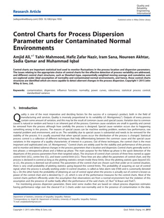
  • 4. robustness of the estimators are found. It is observed that from all the loss functions Tn has smallest SGES than all the competitors whereas Bn is the close competitor to the Tn. To have more global view of the robustness of estimators, 5 × 10⁴ samples X are generated from standard normal distribution, and computed EIF is computed at x = À 4. The boxplots of EIF for n = 3, 7, 15 are given in Figure 1. A couple of observations noted are as follows: Table I. Properties of dispersion statistics under normal and contaminated distributions Distributions n SV RE S Spw Bn Tn AADM S Spw Bn Tn AADM N(0, 1) 3 0.822 0.829 0.910 0.864 0.829 1 1 0.911 0.959 1 7 0.604 0.615 0.789 1.064 0.660 1 1 0.836 0.620 1 15 0.539 0.555 0.675 1.034 0.611 1 1 0.905 0.591 1 C1N3 3 0.931 0.920 1.052 0.953 0.927 0.988 1 0.881 0.973 1 7 0.765 0.712 0.832 1.088 0.729 0.930 1 0.876 0.670 1 15 0.762 0.660 0.714 1.061 0.678 0.867 1 0.949 0.639 1 C5N3 3 1.236 1.198 1.423 1.220 1.204 0.969 1 0.846 0.987 0.805 7 1.201 1.033 0.991 1.163 0.949 0.791 0.919 0.958 0.816 0.833 15 1.308 0.964 0.822 1.120 0.884 0.629 0.853 1 0.789 0.712 C10N3 3 1.437 1.408 1.653 1.404 1.406 0.977 0.997 0.849 1 0.695 7 1.442 1.231 1.186 1.260 1.123 0.779 0.912 0.947 0.891 0.694 15 1.579 1.169 0.953 1.197 1.026 0.603 0.815 1 0.857 0.588 C15N3 3 1.502 1.498 1.716 1.471 1.477 0.979 0.982 0.857 1 0.663 7 1.508 1.323 1.339 1.365 1.207 0.800 0.912 0.901 0.884 0.663 15 1.628 1.273 1.078 1.270 1.108 0.662 0.847 1 0.873 0.597 C20N3 3 1.525 1.493 1.726 1.503 1.501 0.979 1 0.870 0.999 0.652 7 1.503 1.333 1.446 1.448 1.242 0.827 0.932 0.859 0.858 0.666 15 1.565 1.292 1.178 1.339 1.150 0.735 0.890 0.976 0.859 0.639 C1N5 3 1.278 1.261 1.529 1.217 1.238 0.952 0.965 0.796 1 0.769 7 1.307 1.036 0.880 1.105 0.940 0.673 0.849 1 0.851 0.716 15 1.622 0.972 0.731 1.067 0.858 0.451 0.752 1 0.804 0.526 C5N5 3 2.246 2.133 2.735 2.025 2.169 0.902 0.949 0.740 1 0.416 7 2.639 1.947 1.374 1.243 1.647 0.471 0.638 0.904 1 0.286 15 3.252 1.903 0.925 1.160 1.500 0.284 0.486 1 1 0.190 C10N5 3 2.575 2.469 3.053 2.356 2.444 0.915 0.954 0.772 1 0.375 7 2.956 2.322 2.139 1.502 1.992 0.508 0.647 0.702 1 0.255 15 3.369 2.266 1.236 1.293 1.831 0.367 0.546 1 1 0.200 C15N5 3 2.546 2.469 2.951 2.378 2.462 0.934 0.963 0.806 1 0.379 7 2.806 2.356 2.665 1.833 2.071 0.653 0.778 0.688 1 0.315 15 3.029 2.307 1.622 1.446 1.903 0.477 0.627 0.891 1 0.251 C20N5 3 2.428 2.352 2.744 2.327 2.355 0.959 0.989 0.848 1 0.407 7 2.559 2.241 2.849 2.135 2.031 0.794 0.906 0.713 0.951 0.391 15 2.642 2.166 2.015 1.627 1.906 0.616 0.751 0.807 1 0.323 Table II. SGES of various dispersion estimators n L(Y) S Spw Bn Tn AADM 3 E|Y| 5.087 4.152 5.067 2.969 4.305 7 5.819 4.600 3.163 2.247 4.133 15 6.452 4.840 2.736 1.855 4.068 3 Median|Y| 28.687 18.202 30.388 11.390 19.371 7 35.972 21.732 12.729 6.593 17.482 15 43.242 23.731 8.674 4.101 16.745 3 E(Y2 ) 5.086 4.180 5.250 2.756 4.347 7 5.748 4.614 2.897 2.026 4.156 15 6.373 4.847 2.584 1.716 4.080 A. ALI ET AL. Copyright © 2015 John Wiley Sons, Ltd. Qual. Reliab. Engng. Int. 2015
  • 5. • The distribution of EIF of S is much wider than rest of all the estimators. So, S is less resistant to single outlier than all. • The boxplot of Bn is also much wider than AADM, Spw, and Tn, but its median line always lie down to the line of AADM and Spw. • The boxplot of AADM and Spw show the same behavior and are not much wider, and they are found to be much away from the target point zero. So, they are also not much resistant to single outlier. • The boxplot of Tn is not much wider, and its median line lies near to point zero and hence concluded that it is not much effected to single outlier. 3. Control chart structure for the process dispersion This section presents a general framework that helps building dispersion control charts based on various dispersion statistics. Suppose P be a dispersion statistic (one of the aforementioned dispersion statistics) calculated from a subgroup of size n attained from an in-control process. Let Y be a pivotal quantity that explains relative dispersion between the statistic P and the process parameter σ and is evaluated as Y ¼ P σ (similar to W ¼ R σ for R chart). The expected value of Y is E Yð Þ ¼ E P σ ¼ E Pð Þ σ ¼ t2 that completely depends on sample size n. For application point of view, E(P) can be replaced by the average of P ’ s, calculated from a suitable number of random samples generated from an in-control process. An unbiased estimator of σ is thus obtained as σ^¼ P t2 . Mahoney21 and Kao and Ho22 used several non-normal distributions and examined their effect on the values of t2 and Shewhart X and R charts and conclude that the inappropriate use of t2 values increases the FAR of X and R charts. Hence, to avoid such an increase in the FAR, it is a necessity to compute t2 values for different parent environments. There exist two different approaches for building control limits of a dispersion control chart: L-sigma limits (usually L is taken to be 3 or it can be adjusted with false alarm rate) approach and probability limits approach. The use of L-sigma limits becomes inappropriate when the distribution of plotted statistic is not symmetric (cf. Montgomery1 and Ryan23 ). This study utilizes the probability limits approach for the construction of control limits of dispersion charts. Probability limits for the dispersion chart based on statistic P can be computed by using the quantile points of distribution of Y. Let α be the particular probability of making a type-I Table III. Quantile points of Y and value of t2 for charts under normality Y n S Spw Bn Tn AADM Q0.001 3 0.0300 0.025 0.0423 0.0441 0.0248 7 0.2508 0.2206 0.2171 0.1570 0.2274 15 0.4724 0.442 0.4360 0.3152 0.4360 Q0.999 3 2.6212 2.0246 4.1952 4.1241 2.1320 7 1.9259 1.7353 2.4056 2.6708 1.8402 15 1.5929 1.5233 1.7793 1.9453 1.6125 t2 3 0.8857 0.6651 1.2979 1.3237 0.7084 7 0.9602 0.8586 1.0696 1.0704 0.879 15 0.9833 0.9338 1.0308 1.0134 0.9463 Figure 1. Boxplot of EIF(x, P, X) A. ALI ET AL. Copyright © 2015 John Wiley Sons, Ltd. Qual. Reliab. Engng. Int. 2015
  • 6. error and Yα be the α-quantile pot of the distribution of Y. When the in-control σ is known, the process dispersion can be monitored by plotting statistic P on the dispersion control chart with respective lower probability limit and upper probability limit. The probability limits for the dispersion chart based on statistic P are given in the following: LCL ¼ Yα 2 σ with Pr Y ≤ Yα 2 ¼ α 2 UCL ¼ Y 1Àα 2ð Þ σ with Pr Y ≤ Y 1Àα 2ð Þ ¼ 1 À α 2 In practice, the in-control process dispersion σ is usually unknown and therefore has to be estimated. Then, the probability control limits are given below: LCL ¼ Yα 2 P t2 with Pr Y ≤ Yα 2 ¼ α 2 UCL ¼ Y 1Àα 2ð Þ P t2 with Pr Y ≤ Y 1Àα 2ð Þ ¼ 1 À α 2 Note that the quantile points in aforementioned probability control limits are not necessarily the same and might be different in previous expressions even when the probability of making a type-I error is the same. For a parent environment, the α 2 À Áth and 1 À α 2 À Áth quantile points of the distribution of Y depend completely upon subgroup size n for every choice of P. On the same way, the use of quantile points that have been calculated under the assumption of normality is unsuitable for adjusting probability limits for processes following contaminated distributions. Therefore, these quantile points must also be computed by giving proper consideration to the parent environments. Monte Carlo simulation is used for the computation of t2 and quantile points. The values of t2 and quantile points for some particular values of n are given in Table III. Any plotting statistic P falling outside its respective probability control limits indicates that the process is out of control and needs corrective actions that bring it back into in-control state. For the rest of the study, we will refer to the control charts based on S, AADM, Spw, Bn and Tn as S chart, AADM chart, Spw chart, Bn chart and Tn chart, respectively. 4. Performance evaluation of the proposed dispersion control charts To assess the performance of the proposed dispersion control charts, power (1À β) of the control chart has been used as a performance measure. Power curves provide useful information on the detection capability of the dispersion control charts. Performance under normality: The performance is measured under normal and contaminated normal environments. Using structure given in previous section, probability control limits are computed for varying values of n, and the power of the proposed dispersion control charts is evaluated under uncontaminated and contaminated normal environments. For the power computations, shifts in the process dispersion parameter σ have been considered in terms of δσ. If δ = 1, process dispersion is in-control and if δ 1, the process dispersion is out-of-control. The powers of the dispersion control charts for different values of sample size (n) and UCL = 0.002 are provided in Table IV. It can be seen under uncontaminated environment that the dispersion S chart has the largest power among all its competitors, whereas Spw chart behaves similar to S chart. When n=7, the S chart has 16% chance to detect a shift of 1.947 σ in the process, whereas Bn chart has 12.5% chance which is the smallest among all charts. For the small sample, the performance of Tn is better than Bn vice versa for the large sample. Performance under contaminated environments: Performance of control charts, in previous section, was assessed under the ideal assumption of normality. In practice, quality characteristics (e.g., purity of the water, capacitance, insulation resistance, and surface finish, roundness, mold dimensions, and customer waiting times, impurity levels in semiconductor process chemicals, and beta particle emissions in nuclear reaction) from more real-world processes follow non-normal and contaminated distributions (cf. Hurdey and Hurdey,24 Bissell,25 James26 and Miller and Miller27 ). Hence, in these circumstances (and many others), it is not suitable to employ the control charts depend upon the assumption of normality, and therefore, there is a necessity to revise the evaluation of different variability charts for non-normal distributions and contaminated distributions. The performance of the proposed dispersion charts is investigated for a variety of contaminated distributions by using the limits based on normality, and results are evaluated in terms of relative change from the nominal value FAR following by the Human et al.28 This will give departure of the observed FAR from the nominal value. The relative change (RC) can be calculated as A. ALI ET AL. Copyright © 2015 John Wiley Sons, Ltd. Qual. Reliab. Engng. Int. 2015
  • 7. TableIV.Powersofdispersionscontrolchartsundernormaldistributionwhenα=0.002 δ n 3715 SSpwBnTnAADMSSpwBnTnAADMSSpwBnTnAADM 10.0020.0020.0020.0020.0020.0020.0020.0020.0020.0020.0020.0020.0020.0020.002 1.3160.0190.0160.0150.0160.0180.0420.0450.0280.0230.0370.1000.1090.0780.0480.078 1.6320.0770.0660.0570.0630.0710.2030.2060.1320.1020.1760.4760.4870.3810.2460.398 1.9470.1640.1480.1250.1370.1540.4260.4290.3010.2310.3810.7910.7960.6940.5010.723 20.1800.1630.1380.1510.1690.4610.4650.3320.2540.4160.8250.8300.7330.5410.761 2.2630.2620.2430.2040.2270.2490.6180.6210.4770.3750.5710.9310.9330.8720.7030.895 2.5790.3560.3340.2890.3150.3430.7560.7560.6230.5060.7140.9790.9790.9490.8320.963 2.8950.4400.4180.3670.3980.4260.8460.8450.7320.6140.8120.9930.9930.9790.9050.987 30.4650.4440.3910.4240.4520.8670.8660.7610.6450.8360.9950.9950.9850.9220.991 3.2110.5120.4910.4390.4730.4990.9010.9010.8100.6990.8760.9980.9980.9920.9460.996 3.5260.5750.5540.5030.5360.5620.9360.9350.8640.7650.9160.9990.9990.9960.9690.998 3.8420.6260.6090.5590.5890.6160.9580.9570.9010.8160.9441.0001.0000.9980.9810.999 40.6500.6320.5850.6140.6400.9660.9640.9160.8350.9531.0001.0000.9990.9850.999 4.1580.6710.6540.6080.6350.6610.9720.9710.9280.8530.9611.0001.0000.9990.9891.000 4.4740.7090.6930.6500.6760.7000.9810.9800.9470.8830.9731.0001.0001.0000.9921.000 4.7890.7410.7260.6850.7100.7320.9860.9860.9610.9040.9811.0001.0001.0000.9951.000 50.7590.7460.7070.7300.7510.9890.9890.9670.9170.9851.0001.0001.0000.9961.000 60.8260.8160.7850.8030.8190.9960.9960.9850.9550.9941.0001.0001.0000.9991.000 A. ALI ET AL. Copyright © 2015 John Wiley Sons, Ltd. Qual. Reliab. Engng. Int. 2015
  • 8. RC ¼ ^α À α α * 100 where α is the observed FAR and α is the nominal value for the FAR (cf. Human et al.28 ). The results of RC are presented in Table V. From Table V, it can clearly be shown that there is significant increase in observed FAR according to the nominal value of the FAR and this tendency depends upon the estimator and this behavior is observed for small and large levels of contamination. All the estimators are badly affected by the contamination. It can observed that Tn, AADM and Bn shown smaller changes from the nominal value for smaller as well as large sample sizes. But with the increase in contamination level, the observed FAR of control charts based on S and Spw estimators increase rapidly from the nominal value of α. 4.1. Comparison of Shewhart-type, cumulative sum, and exponentially weighted moving average charts Shewhart-type control charts are used to detect large shifts in the process parameter and are less effective for the small shift detection. CUSUM by Page29 and EWMA by Roberts30 are termed as memory type control charts and are used to detect small and moderate shifts. For comparisons purposes, the performance of CUSUM and EWMA is also evaluated. Average run length (ARL) is used as a performance measure. Assuming that process is in-control state and Pj be the sample dispersion statistic based on jth sample of size n. CUSUM structure is given as Cþ j ¼ max 0; Pj À K1 þ Cþ jÀ1 h i and CÀ j ¼ max 0; ÀPj À K1 þ CÀ jÀ1 h i where j = 1, 2 …. and K1 is the reference value. While initial value is Cþ o ¼ CÀ o ¼ σo and σo is target value. If Cþ j or CÀ j is greater than h (decision limit), then CUSUM chart will produce an out of control alarm at first jth sample. The control limits h of the CUSUM is determined to fix ARL at some specified value, and performance of this chart totally depends on the value of K1 and h.(cf. Tupra and Ncube31 and Nazir et al.32 ). Exponentially weighted moving average control chart that allocates exponentially decreasing weights to the observations EWMA structure can be defined as zj ¼ λPj þ 1 À λð ÞzjÀ1; j ¼ 1; 2; 3; …: where λ is the smoothing parameter and zo = σo. The EWMA chart respond out of control if Zj falls above or below the following limits: UCL=LCL ¼ E Pð Þ ± LσP ffiffiffiffiffiffiffiffiffiffiffiffiffiffiffiffiffiffiffiffiffiffiffiffiffiffiffiffiffiffiffiffiffiffiffiffiffiffiffiffiffi λ λ À 2 1 À 1 À λð Þ2j h ir j ¼ 1; 2; 3…: where L 0 determines the width of limits and is set to satisfy ARL at some specific value. (cf. Lucas and Saccucci33 ). Table V. RC under contaminated environments with α = 0.002 and δ = 0 n ε K 3 5 S Spw Bn Tn AADM S Spw Bn Tn AADM 3 1 190.5 184 179 135.5 224.5 590 568 551.5 507 554 5 1145 1057 1028 911.5 1066.5 2763.5 2727 2619.5 2421 2724.5 10 2396 2163 2133 1915.5 2196.5 5634.5 5291 5331 4971.5 5385 15 3567.5 3245 3146.5 2859.5 3280.5 8252.5 7802 7723 7347.5 7937.5 20 4705 4340 4126 3846.5 4399.5 10,776 10,339 10,102 9621 10,463 7 1 518.5 328 83 12.5 217 1277 1106 174.5 38 784.5 5 2592 1942 513.5 164 1224.5 6247.5 5275 1201 318.5 4096 10 5297.5 4161 1393.5 485 2806.5 12,141 10,489 3368 1113.5 8345 15 8023 6710 2622 1007 4726.5 17,203 15,616 6223 2349 13,017 20 10,737 8954 4113.5 1739 6753 22,059 19,989 9681 4079 17,231 15 1 878 428 55 45 174 2537 1656 94.5 30 849 5 4651.5 2707 509 174 1234 11,612 8492 1125 294.5 5274.5 10 9661 6600 1709 506 3561.5 21,349 17,216 3842 1009.5 12,031 15 14,969 11,154 3717 1155 6709 29,060 25,049 7918 2326.5 19,370 20 19,949 15,857 6494.5 2201 10,567 35,346 31,715 13,499 4446.5 26,250 A. ALI ET AL. Copyright © 2015 John Wiley Sons, Ltd. Qual. Reliab. Engng. Int. 2015
  • 9. Rest of the study will refer the CUSUM control charts based on S, AADM, Spw, Bn and Tn as SC chart, AADMC chart, SpwC chart, BnC chart and TnC chart, respectively, as well as for the EWMA control charts as SE, AADME, SpwE, BnE and TnE charts. Table VI presents the control value of Shewhart, EWMA, and CUSUM charts, which set ARL≅370. For the comparison and to investigate the performance of the said charts, λ =0.2 and n=3 are used in this study. Under normality; SC, SPwC, SE, and SPwE control charts are sensitive in detecting small shift. But an abrupt change has been observed AADM chart at δ = 1.5. In the case of 5% level of contamination, SPwE and AADME show inflated ARL at δ =1, and rest of the control charts are badly affected by the contamination of all levels except AADM chart. (cf. Table VII). For the large sample sizes, the performance of Tn chart, TnE and TnC, is observed to be satisfactory for the different contaminations, and at some situations, Bn chart, BnE and BnC, is seen to be close competitors to the Tn chart, TnE and TnC. Likewise to the aforementioned discussion, all AADM chart and AADME shows different behavior for small shift. 5. Conclusions The study explores the performance of several dispersion charts under normal and different contaminated normal processes. For normally distributed quality characteristics, the S chart is superior to the all competitors control charts. It is observed that the Spw chart is similar to that of the S chart under EWMA and CUSUM structures. For the contaminated cases when there is no prior information related to the distribution of the process, AADM and Tn charts based on Shewahrt, CUSUM and EWMA are the better choices than the other charts. The performance of all the control charts based on S control charts is too much affected in the presence of contamination. The use of control charts based on AADM and Tn estimators is recommended when there is contamination in the output of the process. References 1. Montgomery DC. Introduction to Statistical Quality Control (6th edn). Wiley: New York, 2009. 2. Burr IW. The effect of non-normality on the constants for Xe and R charts. Industrial Quality Control 1967; 23:566–569. 3. Braun WJ, Park D. Estimation of for individuals charts. Journal of Quality Technology 2008; 40:332–344. 4. Abbasi SA, Miller A. On proper choice of variability control chart for normal and non-normal processes. Quality and Reliability Engineering International 2012; 28:279–296. Table VII. ARL of dispersion charts under normal and contaminated distributions Control charts σ N(0, 1) C5N3 C15N3 δ 1 1.5 2.579 1 1.5 2.579 1 1.5 2.579 Shewhart S 371.6 19.2 2.7 36.8 9.8 2.4 13.2 5.1 2.0 Spw 369.3 18.7 2.7 36.9 9.7 2.4 13.3 5.1 2.0 Bn 369.7 23.5 3.2 38.7 11.3 2.8 14.1 5.8 2.6 Tn 370.2 20.5 2.9 42.1 10.5 2.6 14.9 5.4 2.1 AADM 369.3 808.5 41.5 311.8 92.5 14.9 198.2 31.5 6.7 EWMA S 372.0 11.7 2.3 60.8 7.4 2.1 15.9 4.3 1.8 Spw 369.8 240.6 4.7 544.0 34.2 3.8 119.8 10.9 2.8 Bn 370.4 10.5 2.6 41.1 7.3 2.3 13.2 4.6 2.0 Tn 370.0 10.2 2.5 45.9 7.2 2.3 14.2 4.5 1.9 AADM 371.8 100.6 3.9 387.4 23.9 3.3 73.2 8.9 2.5 CUSUM S 370.2 10.9 3.5 30.7 10.1 3.4 11.0 6.3 2.9 Spw 370.0 11.1 3.6 49.0 8.3 3.2 15.9 5.6 2.7 Bn 369.7 12.1 3.8 48.6 13.0 3.4 16.2 6.0 2.8 Tn 371.8 11.5 3.7 53.1 8.6 3.3 17.0 5.8 2.7 AADM 369.6 11.0 3.5 48.8 8.2 3.1 15.7 5.5 2.6 EWMA, exponentially weighted moving average; CUSUM, cumulative sum. Table VI. Control limits and parameter values for various dispersion charts Estimator Shewhart EWMA; λ = 0.2 CUSUM LCL UCL L K1 h S 0.038 2.584 7.38 0.996 3.440 Spw 0.0265 1.938 8.9 0.748 2.640 Bn 0.0482 4.06 13.22 1.457 5.6227 Tn 0.05 3.97 11.12 1.487 5.44 AADM 0.0415 4 8.16 0.797 2.73 A. ALI ET AL. Copyright © 2015 John Wiley Sons, Ltd. Qual. Reliab. Engng. Int. 2015
  • 10. 5. Jensen WA, Jones-Farmer LA, Champ CW, Woodall WH. Effects of parameter estimation on control chart properties: a literature review. Journal of Quality Technology 2006; 38:349–364. 6. Rocke DM. Robust control charts. Technometrics 1989; 31:173–184. 7. Rocke DM. Xe Q and RQ charts: robust control charts. The Statistician 1992; 41:97–104. 8. Tatum GL. Robust estimation of the process standard deviation for the control charts. Technometrics 1997; 39:127–141. 9. Vargas JA. Robust estimation in multivariate control charts for individual observations. Journal of Quality Technology 2003; 35:367–376. 10. Davis CM, Adams BM. Robust monitoring of contaminate data. Journal of Quality Technology 2005; 37:163–174. 11. Riaz M, Saghir A. A mean deviation-based approach to monitor process variability. Journal of Statistical Computation and Simulation 2008; 79:1173–1193. 12. Bickel PJ, Lehmann EL. Descriptive statistics for non-parametric models III: dispersion. The Annals of Statistics 1976; 4:1139–1158. 13. Croux C, Rousseeuw PJ. Time efficient algorithms for Two highly robust estimators of scale. Computational Statistics; 1, Y. Dodge; J. Whittaker, Physika-Verlag: Heidelberg, 411–428. 14. D’Agostino RB. Linear estimates of the normal distribution standard deviation. American Statistician 1970; 23:14–15. 15. Muhammad F, Ahmad S, Abiodullah M. Use of probability weighted moments in the analysis of means. Biometrical Journal 1993; 35:371–378. 16. Rousseeuw PJ, Croux C. Alternatives to the median absolute deviation. Journal of the American Statistical Association 1993; 88:1273–1283. 17. Hampel FR. The influence curve and its role in robust estimation. American Statistical Association 1974; 69(346):383–393. 18. Huber PJ. Robust Statistics. Jhon wiley: New York, 1981. 19. Hampel FR, Ronchetti EM, Rousseeuw PJ, Stahel WA. Robust Statistics: The Approach Based on Influence Functions (Vol. 114). John Wiley Sons: New York, 2011. 20. Croux C. Limit behavior of the empirical influence function of the median. Statistics probability letters 1998; 37(4):331–340. 21. Mahoney JF. The influence of parent population distribution on d2 values. IIE Transactions (Institute of Industrial Engineers) 1998; 30:563–569. 22. Kao SC, Ho C. Robustness of R-chart to non-normality. Communications in Statistics, Simulation and Computation; 36 pp:1089–1098. 23. Ryan TP. Statistical Methods for Quality Improvement (2nd edn). Wiley: New York, 2000. 24. Hrudey SE, Hrudey EJ. Safe Drinking-water. Lessons from Recent Outbreaks in Affluent Nations. IWA Publishing: London, UK, 2004. 25. Bissell D. Statistical methods for SPC and TQM (1st edn). Chapman Hall: New York, 1994. 26. James PC. CPK equivalencies. Quality 1989; 28:75. 27. Miller I, Miller M. Statistical Methods for Quality with Applications to Engineering and Management. Prentice-Hall, Inc.: Englewood Cliffs, NJ, 1995. 28. Human SW, Kritzinger P, Chakraborti S. Robustness of the EWMA control chart for individual observations. Journal of Applied Statistics 2011; 38:2071–2087. 29. Page ES. Cumulative Sum charts. Technometrics 1951; 3(1):1–9. 30. Roberts SW. Control chart tests based on geometric moving averages. Technometrics 1959; 1(3):239–250. 31. Tuprah K, Ncube M. A comparison of dispersion quality control charts. Sequential Analysis 1987; 6(2):155–163. 32. Nazir HZ, Riaz M, Does RJ. Robust CUSUM control charting for process dispersion. Quality and Reliability Engineering International 2015; 31(3):369–379. 33. Lucas JM, Saccucci MS. Exponentially weighted moving average control schemes: properties and enhancements. Technometrics 1990; 32(1):1–12. Authors' biographies Amjid Ali completed his BS (Hons) Statistics with distinction (Silver Medalist) from the Department of Statistics, University of Sargodha (UoS), Sargodha, Pakistan. After completion of BS (Hons) Statistics, he served the Department of Statistics, UoS, as a teaching Assistant for 3 years. Currently, he is pursuing his MPhil from the Department of Statistics, University of Sargodha, Sargodha, Pakistan. His research interests are statistical process control, nonparametric techniques, and robust methods. He may be contacted at amjidalizafar@gmail.com. Tahir Mahmood obtained his BS (Hons) Statistics with distinction (Gold Medalist) from the Department of Statistics, University of Sargodha (UoS), Sargodha, Pakistan. He served the Department of Statistics, UoS, as a teaching Assistant for 2 years. Currently, he is pursuing his M.Phil from the Department of Mathematics and Statistics, King Fahd University of Minerals and Petroleum, Dhahran, Saudi Arabia. His research interests are statistical process control and nonparametric techniques. His email address is rana. tm.19@gmail.com. Hafiz Zafar Nazir obtained his MS in statistics from the Department of Statistics, Quaid-i-Azam University (QAU), Islamabad, Pakistan, in 2006, and MPhil in statistics from the Department of Statistics, Quaid-i-Azam University, Islamabad, Pakistan, in 2008. He received his PhD in statistics from the Institute for Business and Industrial Statistics (IBIS), University of Amsterdam, The Netherlands, in September, 2014. He is serving as assistant professor in the Department of Statistics, University of Sargodha (UoS), Pakistan. His current research interests include statistical process control, nonparametric techniques, and robust methods. His e-mail address is hafizzafarnazir@yahoo.com. Iram Sana is currently serving as Lecturer in the Department of Statistics, University of Sargodha, Sargodha (UoS), Pakistan. She is currently completing her MPhil in statistics from the Department of Statistics, University of Sargodha, Sargodha, Pakistan. Her research interests are applications of statistical methods. Noureen Akhtar is serving as Assistant Professor in the Department of Statistics, University of Sargodha, Sargodha (UoS), Pakistan. She completed her MPhil in statistics from the Department of Statistics, Bahauddin Zakariya University, Multan, Pakistan. Her research interest is econometric modeling. Sadia Qamar is serving as Lecturer in the Department of Statistics, University of Sargodha (UoS), Sargodha, Pakistan. She completed her MPhil in statistics from the Department of Statistics, Quaid-i-Azam University (QAU), Islamabad, Pakistan. Her research interests are Bayesian analysis and time series modeling. Muhammad Iqbal is serving as Professor and Chairman in the Department of Statistics, University of Sargodha (UoS), Sargodha, Pakistan. He completed his PhD in statistics from the Government College University Faisalabad, Faisalabad, Pakistan. His research interest is econometric modeling. A. ALI ET AL. Copyright © 2015 John Wiley Sons, Ltd. Qual. Reliab. Engng. Int. 2015