Desing and Development of a Steady State System Simulator

THREE CAREER EPISODES
1. DESIGN AND DEVELOPMENT OF A STEADY STATE SYSTEM
SIMULATOR
1.1 INTRODUCTION
CE 1.1. This project was made in order to get my degree as Chemical Engineer. Me and
other two students developed a Steady State System Simulator to be applied in Personal
Computers at the University of America in Bogotá, Colombia. The project was lead by
the Chief of the Computing Department of ECOPETROL, the Colombian Oil
Company that belongs to the Colombian State.
1.2 BACKGROUND
CE 1.2. Processes simulation through computing models was clearly becoming one of
the major tools to do mass and energy balances, that Chemical Engineers apply to
design and optimize processes in the mining and petrochemical industry, allowing not
destructive tests and avoiding pilot plants, saving materials, energy, avoiding potential
accidents, and not generating wastes. Computers applied to Process Engineering has
become one of the main branches of the Chemical Engineering.
CE 1.3. As a main objective we developed the Steady State System Simulator –
SIMPRES to model the following Equipment Processes:
1. Pumps
2. Compressors
3. Heat Exchangers
4. Mixers
5. Splitters
6. Fractionators
7. Reactors
8. Absorption Towers
9. Distillation Towers
10. Flash Distillatory
11. Valves
12. Turbines
13. User’s Module

CE 1 Alvaro H. Pescador 2
CE 1.4 I was in charge of fully developing the simulation modules of Pumps,
Compressors, Heat Exchangers, Valves and Turbines.
CE 1.5. On the other hand, SIMPRES had a bank of 471 compounds including must of
Hydrocarbon used in the Petrochemical Industry both sutured and not sutured, linear
and not linear, as well as inorganic gases such as the H2, CO, CO2, NO, NO2, SO2, SO3,
NH3, and the water.
CE 1.6. The following physicochemical and thermodynamic properties were possible to
compute for mixtures up to 10 compounds, to a given condition of Pressure,
Temperature and composition (P, T, X):
1. Overall Molecular Weigh
2. Density
3. Overall Heat Capacity
4. Enthalpy
5. Boiling point
6. Dwelled point
CE 1.7. I was in charge of developing the Thermodynamic and Physicochemical
algorithms for computing these properties by using State Equations of Redlich Kwong1
,
and Peng-Robinson2
.
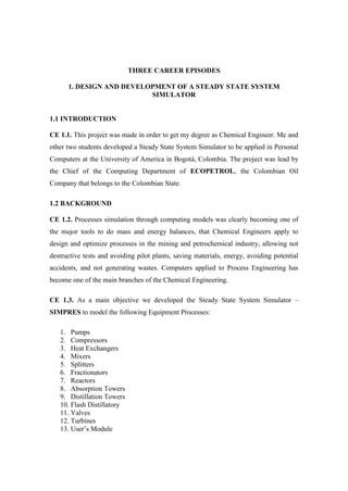
CE 1.8 Overall Project’s Architecture and main Program’s objectives are shown in
Figure 1 in the following page.
1
REID R, PRAUNITZ J. and SHERWOOD T., “The Properties of the Gases and Liquids”, New York,
McGraw Hill, 3a ed, 1977.
2
PENG D.Y., AND ROBINSON D.B., “A New Two Constant Equation of State”, Chemical Engineering
Vol. 15, 1976, p. 59.

CE 1.8 Figure 1. Structure of the Steady State System Si mulator – SIMPRES
1. Pumps
2. Compressors
3. Heat Exchangers
4. Mixers
5. Splitters
7. Reactors
6. Fractionators
9. Distillation
Towers
8. Absorption /
Desortion
Towers
11. Valves
12. Turbines
Calls PROPERTY to
characterize OUTPUT
Streams
10. Flash
13. User´s
Module
COMPOUNDS DATA
BANK
Matrix of 471 Compounds
with 14 Physicochemical
parameters of pure
Substances (Appendix 2)
PRINTER
Shows the OUTPUT DATA
through the screen, or by a
Printed form:
 Process Topology
 Input and Output Equipment’s
Simulation Parameters.
 P, T, M, X conditions of the
process Streams.
 Warning Messages
READER
Asks and validates INPUT DATA
to the user:
 System Unit, British or International
 Compounds Codes, up to 471.
 Equipment’s Simulation Parameters
 P,T,M,X conditions of Input streams
up to 10 compounds.
PROPERTY
By Using Equations of
State Calls The Bank
which have parameters
of 471 pure compounds,
to compute
Physiochemical and
Thermodynamic
properties of Input
and Output Streams.
SIMPRO
Executive Program
 Calls PROPERTY
to characterize
Input Streams.
 Calls the Equipment
Simulation Modules in
agreement with the
specified Process Topology.
 Calls CSL, Convergence
Simulation Loop
if recycling streams are
found, in agreement with
the process Topology
1. Pumps
2. Compressors
3. Heat Exchangers
4. Mixers
5. Splitters
7. Reactors
6. Fractionators
9. Distillation
Towers
8. Absorption /
Desortion
Towers
11. Valves
12. Turbines
Calls PROPERTY to
characterize OUTPUT
Streams
10. Flash
13. User´s
Module
COMPOUNDS DATA
BANK
Matrix of 471 Compounds
with 14 Physicochemical
parameters of pure
Substances (Appendix 2)
PRINTER
Shows the OUTPUT DATA
through the screen, or by a
Printed form:
 Input and Output Equipment’s
Simulation Parameters.
 P, T, M, X conditions of the
process Streams.
 Warning Messages
READER
Asks and validates INPUT DATA
to the user:
 System Unit, British or International
 Compounds Codes, up to 471.
 Equipment’s Simulation Parameters
 P,T,M,X conditions of Input streams
up to 10 compounds.
PROPERTY
By Using Equations of
State Calls The Bank
which have parameters
of 471 pure compounds,
to compute
Physiochemical and
Thermodynamic
properties of Input
and Output Streams.
SIMPRO
Executive Program
 Calls PROPERTY
to characterize
Input Streams.
 Calls the Equipment
Simulation Modules in
agreement with the
specified Process Topology.
 Calls CSL, Convergence
Simulation Loop
if recycling streams are
found, in agreement with
the process Topology

1.3. PERSONAL WORKPLACE ACTIVITY
CE 1.9. I was in charge to identify the grades of freedom3 for each one of the
Equipment modules in Figure 1. It means that for simulation purposes of Steady State
Operations, the package should ask as few data to the user as it would be
mathematically possible. The P,T,M,X conditions of inputs streams must always be
defined by the user.
CE 1.10. Pumps. It was very important to secure the information introduced to the
system. In an input stream to a pump I must be secure that at the P1,T1,M1,X1 conditions
of a pure compound, or mixture, it is in a liquid state. If not, a warning message is given
to the user.
Figure 2. Simulation Parameters for Pumps
CE 1.11 The output conditions of Temperature, T2 and Enthalpy, H2, are computed, in
agreement to a desirable output pressure, P2. The Work, W, necessary to do the job is
computed by the module. Another option is to supply the Work value, W, and then P2
will be computed by SIMPRES. In any case, the Pump’s efficiency, η, must be
provided by the user.
CE 1.12. Compressors. At P1,T1,M1,X1 conditions of a pure compound, or a mixture,
the input stream must be a gas. If not, a warning message is given to the user. The user
may choose between an adiabatic or a polytrophic compression. In the first case an
efficiency, η, must be provided, in the second is computed by the module as a result, in
agreement to a compression factor, Cf, or a desirable output pressure, P2.
3
PERRY, Robert E and CHILTON, Cecil, “Chemical Engineering Handbook”, Mexico, McGraw-Hill,
1984, Vol. 1, Simulation System Processes p. 2-73.
PP1,T1,M1,X1
P2,T2,M2,X2
W
η

Figure 3. Simulation Parameters for Compressors
CE 1.13 As output values the simulator find the kind of Eliot compressor needed,
number of Stages, pressure and temperature of the output stream, as well as W, the job
needed to compress the gas, following a polytrophic compression curve. If an adiabatic
(ideal) compression was chosen, only W is computed, as well as the characteristics of
the output stream.
CE 1.14. Heat Exchangers. SIMPRES has two categories of Equipments:
a. Heat Exchangers of Service. They can be either coolers or heaters, condensers or
boilers. To simulate them it is necessary to specify two streams in the equipment’s
topology: those which manage the process fluid, as shown in figure 4. The process
fluid is the fluid which is about to be condensed, cooled, heated or boiled. To
provide the heat, Q, SIMPRES uses water as service stream in the case of coolers
and condensers, and steam in the case of heaters and boilers.
Figure 4. Heat Exchangers of Service
CCP1,T1,M1,X1 P2,T2,M2,X2
W
η
Cf
HE
S-2
HE
S-2
HE
S-2
HE
C-1
HE
C-1
Condenser Heater
Process Fluid
Q
-Q

b. Heat Exchangers of Process. They can also be coolers or heaters, condensers or
boilers. To simulate them, it is necessary to specify four streams in the equipment’s
topology: those which manage the process fluid, and those which manages the
service fluid. The hot fluid must be taken as the process fluid, and its stream be
defined first in the input and output topology of the heat exchanger, as shown in
figure 5. Calculations for the energy balance are shown in Appendix 1.
Figure 5. Heat Exchangers of Process
c. Parameters. SIMPRES allows to simulate the following kind of heat exchangers:
1. Double Pipe heat exchanger, fluids in parallel or counter stream (A, UD, DPP,
DPS).
2. 1-1 Heat Exchanger (A, UD, DPP, DPS).
3. Pipes-Shell Heat Exchanger (A, UD, NSP, NSS, DPP, DPS).
4. Coolers and Heaters (Q, OTPF, DPP, DPS).
5. Condensers (Q, X, Tb, Dsub, DPP, DPS).
6. Boilers (Q, X, Tr, Dsob, DPP, DPS).
CE 1.15 The user must provide the parameters in parenthesis. Boldfaced parameters
means simulation can be done by using any of them, the one user may know or
estimate easier. The following is the list of the parameters defined above. As can be
seen, SIMPRES allows to work units in the British System or in the International one,
but once a Unit System is chosen all the units must be worked on it:
t4
3 T3T1 1 HE
P-1
2
4
t2
Process Fluid: T1 > T3
T1 > t2

A: Heat Exchange Area (ft2
, or m2
)
UD: Total Dirty Coefficient of Heat Exchange (Btu / hr ft2
°F, or Kcal / hr m2
°C)
DPP: Lost Pressure in the fluid of Process (Psi, or atm)
DPS: Lost Pressure in the fluid of Service (Psi, or atm)
NSP: Number of Steps, pipe side.
NSS: Number of Steps, shell side.
Q: Heat given by the hot fluid, (Btu/lb, or Kcal / Kg).
OTPF: Output Temperature of the Process Fluid. (°F or °C).
X: Vapor Relation at condenser or boiler output (when a partial condensation or
partial evaporation is desired).
Tb: Specifies condensed at boiling point, (°F or °C).
Dsub: Specifies condensed sub cooled with a determined delta of temperature, under
its boiling point, (°F or °C).
Tr: Specifies total evaporation, at Dwelt point, (°F or °C).
Dsob: Specifies steam overheated with a determined delta of temperature over its
dwelt point, (°F or °C).
CE 1.16. The exchangers 1 to 3 are Heat Exchangers of Process for operations with
out change of phase, while exchangers 4 to 6 are able to simulate operations with or
with out change of phase, and can be defined either as Heat Exchanger of Service or
of Process. In the last case, the module computes the heat transferred with an energetic
balance over the Process Stream (Hot Fluid in the Appendix 1, Eq. A-1.1). The
temperature of the fluid of service can be established then by using the heat balance Eq.,
A-1.3 of the Appendix 1.
CE 1.17. Mixers. A maximum amount of 6 input streams are allowed, and only one
output stream, as shown in Figure 6.
Figure 6. Mixers
M
.
.
.
.
1
n
M
.
.
.
.
1
n
2 ≤ n ≤ 6

It is not necessary to ask parameters to the user to run this module. By specifying the
codes of input streams (with P,T,M,X conditions defined), and the code of the resulting
or output stream, the mass and energy balance can be done4
.
CE 1.18. Splitters. One single input stream is accepted to feed the splitter and a
maximum of six output streams might be defined, as shown in Figure 7:
Figure 7. Splitters
As simulation parameters the module ask the molar fraction of the input stream which
will conform each one of the output streams (e.g. for tree output streams: 0,3 for the
output stream 1, 0,3 for the output stream 2, and 0,4 for the output stream 3). The total
amount of fractions provided is validated and must be equal to one5
, if not, a warning
message is given to the user.
4
HIMMELBLAU, David, “Basic Principles and Calculations in Chemical Engineering”, Prentice-Hall,
1974, section 2.2, analysis program to solve mass balance problems. Taking from the Spanish
translation, Mexico, CECSA, 1982, p. 99-104.
5
HIMMELBLAU, David, Ob. Cit, p. 102.
S
.
.
.
.
1
n
2 ≤ n ≤ 6

CE 1.19. Reactors. Only one input stream to the reactor and one output stream from it
are allowed, as shown in Figure 8. The estequeometry coefficients of reactives and
products are asked to the user as input parameters (a cero must be provided for
compounds which does not take part in the reaction).
Figure 8. Reactors
CE 1.20. For the reactants, the fraction that is not consumed during the reaction is
asked, thus, for each one of the reactives, the fraction in the products stream is asked.
Optionally, the enthalpy of the reaction may be provided, and must be introduced as
negative, if the reaction is exothermic. Otherwise, it will be computed by the module.
CE 1.21. In a Steady State System Simulator the reactor module takes care about the
mass and energy balance in agreement with reaction’s estequeometry and does not
model kinetic of reaction. To perform kinetic calculations it would be necessary to
consider the time as a process variable6
and that is beyond the boundaries of Steady
State System Simulation7
.
CE 1.22. If in the real process there is more than one stream feeding the reactor, a mixer
must be put before the reactor to run the simulation, and the output stream from the
mixer must feed the reactor.
6
LEVENSPIEL, Octave, “Chemical Reaction Engineering”, Jhon Wiley and Sons Inc, New York, 1980.
Taken form the Spanish Edition, Barcelona, Ed. Reverté, 1986, p. 3-7.
7
PERRY, Robert E and CHILTON, Cecil, “Chemical Engineering Handbook”, Mexico, McGraw-Hill,
1984, Vol. 1, Simulation System Processes p. 2-105.
RR
∆HR
aX + bY cZ

CE 1.23. Fractionation Towers. Six input streams to the tower and six output streams
from it are allowed, as shown in Figure 9.
Figure 9. Fractionation Towers
For the output streams, as simulation parameters SIMPRES ask the distribution factor
for each one of the compounds present in the input stream(s), as well as the desirable
output temperature of the leaving streams. This simulation module can be use to
perform quick mass and energy balance for multi components separation processes in
stages columns, with several feedings and several retirements. As simulation result,
besides the separation, the heat necessary to perform the operation is computed.
CE 1.24 Absorption and Desorption. Six input streams to the tower and six output
streams from it are allowed, as shown in Figure 10. Simulation is done by using the
Wang-Henke method originally developed for distillation8
. As shown in Figure 10, at
least one liquid and one gas inputs streams completely defined (P,T,M,X conditions)
should go inside the tower (maximum 6).
8
WANG and HENKE, “Tridiagonal Matrix for Distillation”, Hydrocarbon Processing, Vol. 6, p. 155,
1966.
FCFC
.
.
.
.
.
.
.
.
.
..
.
Q
.
.
.
.
.
.
FT

Figure 10. Absorption Towers
CE 1.25. The user must provide the following parameters:
1. Tower’s Pressure
2. Number of Stages, N
3. Top Temperature
4. Bottom Temperature
5. Number of vapor retirements
6. Number of liquid retirements
7. Number of Heat Exchangers (in any stage, maximum 6)
8. If there are lateral feedings, the feeding stage.
9. If there are lateral retirements, the retirement stage, the Flow and a code for the
retirement stream.
10. If there are heat exchangers, the stage number and the calorific charge.
CE 1.26. Parameters 3 and 4 are the simulation key, since they set the tower’s
temperature range, and are used to create polynomials to compute the Enthalpy and the
Equilibrium constants, Keq., which will varies between these range. The module
computes mass transfer in each equilibrium stage and as final result provides the
(P,T,M,X) condition of the liquid L', and vapor stream, G', leaving the tower.
AA
.
.
.
.
.
.
.
.
L
G
AA
.
.
.
.
.
.
.
.
AA
.
.
.
.
.
.
.
.
L
GL'
G'

CE 1.27 Distillation Towers. Distillation Columns for separation of multi components
can be run in SIMPRES by using the shortcut method of Smith-Brinkley9
or the
rigorous of Wang Henke. In the first case, only one feeding stream is allowed, F,
(P,T,M,X conditions known). The output streams are the Distillated, D, and the
Residue, R, at the bottom of the column, as shown in Figure 11.
Figure 11. Distillation Towers
CE 1.28 To do the simulation the following parameters must be provided:
2. Number of Stages, N.
3. Number of the feeding stage
4. Reflux relation: L / D
5. Compound’s distribution factors to the top stream. These are the key simulation
parameters since they set the Distillated flow and the temperature profile range.
CE 1.29 The boiler at the bottom of the model must be numbered as stage one. The
method is not restrictively applicable to a column with a partial condenser due to it does
not make a difference between the top stream composition and the one of the Reflux, L.
The effect of a condenser can be estimated by increasing N in 1, as another stage. The
9
SMITH AND BRINKLEY, American Institute of Chemical Engineering, Journal 6, 446, 1960.
HE
C-1
HE
B-1
DT
D
R
F
L
HE
C-1
HE
B-1
DT
D
R
F
L

final values of TN+1 and T1 are the Dwelt point of the computed top’s product and the
boiling point of the computed bottom’s product, respectively. The presence of the
boiler and the condenser are included in the model: they DO NOT have to be specified
apart from the model.
CE 1.30 By the Wang Henke Method, six input streams are allowed as well as 6 out put
streams: the Distillated, the Residue and four lateral retirements. The following
parameters must be provided by the user:
2. Number of Stages, N
3. Distillated Flow, D
4. Reflux relation: L / D
5. Top Temperature
6. Bottom Temperature
7. Number of vapor retirements
8. Number of liquid retirements
9. Number of Heat Exchangers (in any stage, maximum 6)
10. Distillated Vaporization Ratio (from 0 to 1)
11. Distillated stream code.
12. If there are lateral feedings, the feeding stage.
13. If there are lateral retirements, the retirement stage number, flow, and code of
the retirement stream.
14. Heat exchangers: the stage number and the calorific charge.
CE 1.31. Flash. One feeding stream is allowed, F, (P,T,M,X conditions known) being
the output streams the Gas phase, G, and the Liquid phase, L, at the bottom of the
column, as shown in Figure 12.

Figure 12. Flash
Flash module can be used to split a stream in its liquid and vapor phases
instantaneously, in one single stage. Top Stream leaves the splitter as a gas at its dwelt
point, while bottom stream leaves it as liquid at its bubble point.
CE 1.32. Valves. One input stream to the valve and one output stream from it, are
allowed, as shown in figure 13. As simulation parameter the pressure drop caused by the
valve is asked to the user. Temperature of the output stream is computed through an
adiabatic flash.
Figure 13. Valves
CE 1.33. Turbines. One input stream to the turbine and one output stream from it, are
allowed, as shown in figure 14. Either P2 or W is asked to the user as simulation
parameter. In any case as an additional parameter the isentropic efficiency, η, also must
be provided by the user:
FLFL
F
G
L
FLFL
F
G
L
VV
∆P
R
P1 P2
P2 < P1

Figure 14. Turbines
following the first law of the Thermodynamics10
, the internal energy of the gas slows
down in agreement to the Job provided by the system, therefore the output temperature
of the gas might be very low, allowing the turbine to act as a refrigerant. The output
temperature is estimated as is the expansion would be made at constant entropy. In
agreement with the second law of Thermodynamics this is an idealization (a reversible
an adiabatic process)11
. The real Job WR is finally computed based upon the isentropic
efficiency.
CE 1.34 User’s Module. Modules designed by the user may have up to 6 input and 6
output streams, as shown in Figure 15:
Figure 15. User’s Modules
up to 18 parameters may be introduced by the user for simulation purposes. Figure 14
must be regarded as a Control Volume12
of a Steady State Process. Module’s purpose is
to establish output stream conditions in agreement with an energy and mass balance of
10
SONNTANG AND VAN WYLEN, “Introduction to the Thermodynamics: Classical and Statistical”,
New York, John Wyley and Sons Inc., 1971. Taken from the Spanish translation, Mexico, Limusa,
1979, p. 156-160.
11
SONNTANG AND VAN WYLEN, Op. cit, p. 255-268.
12
SONNTANG AND VAN WYLEN, Op. cit, p. 38-39.
T
W
TT
W
P2
P1
P2 < P1
η
WR = W * η
UM
.
.
.
n
.
.
.
.
1
n
1 ?n ? 6
-
W
1
.
UM
.
.
.
n
.
.
.
.
1
n
UM
.
.
.
n
.
.
.
.
1
n
.
.
.
.
1
n
1 ≤ n ≤ 6
-Q
W
1
.

the Control Volume, bearing in mind that heat leaving the system Q, must be considered
as negative while introduced to the system as positive. The opposite happens with the
Job W, should the equipment would need or make any Job.
CE 1.35. User’s module can access the PROPERTY library (Figure 1, page 3) of
SIMPRES which allows to estimate physic and thermodynamic properties of Input and
Output streams, in the following ways:
1. Estimates all the properties
2. Computes Bubble Point, °K
3. Computes Dwelt Point, °K
4. Runs Isotermic Flash (outcome: stream vaporization ratio, from 0 to 1, and heat
needed) .
5. Runs Adiabatic Flash (outcome: stream vaporization ratio, from 0 to 1).
6. Computes Gas Compressibility Factor: Z, and gas density (gr / mol-gr).
7. Estimates Enthalpy, Kcal / Kmol
8. Estimates Heat capacity, Kcal / Kmol °K
9. Estimates Equilibrium Constants of pure compounds, Keq.
10. Computes Density, gr / mol-gr
11. Computes Average Molecular Weight, gr / mol-gr
12. Computes output temperature °K for a given enthalpy, (by using adiabatic flash
routine).
CE 1.36. The Simulator SIMPRES was exhaustively tasted for individual equipments,
simple processes and complex processes. Complex processes are those having recycling
streams with equipments conforming loops indented or one internal and the other
external as the one shown on Figure 16.

Figure 16. Simulation Model for a Ciclohexane Production Plant
CE 1.37. The equipments 2, 3 and 4 are conforming a loop since there is a recycling
stream coming from the equipment 4, to the equipment 2. This loop is internal to the
one conformed by equipments, 5, 6, 7, 8 and 1 which integrate an external loop, since
there is a recycling stream coming from the equipment 8 to the equipment 1, whose
output stream feeds the equipment 2. Equipments 10 and 11 are conforming a simple
loop.
CE 1.38. In order to solve this model it is necessary to know P,T,M,X conditions of the
Streams 1 and 3, and to suppose initial values for the P,T,M,X conditions of the
Recycling Streams 2, 5 and 15. After this, SIMPRES ask to the user simulation
Process Equipments
1) Mixer, M-1 7) Splitter, S-1
2) Heat Exchanger of Process, HE P-1 8) Compressor, C-1
3) Heat Exchanger of Service, HE S-1 9) Valve, V-1
4) Reactor, R-1 10) Heat Exchanger of Process, HE P-2
5) Heat Exchanger of Service, HE S-2 11) Fractionation Tower, F-1
6) Flash, F-1 12) Heat Exchanger of Service, HE S-3
1 R-1
FL-1
FT-1
HE
S-1
HE
S-2
HE
S-3
HE
P-1
HE
P-2
C-1S-1
M-1
3
2
4
5
6
7 8
9
10
11
12
13
14
15
16
17 18
19
1 2 3
4
5
6
V-1
7
8
9 10
11
12
1 R-1
FL-1
FT-1
HE
S-1
HE
S-2
HE
S-3
HE
P-1
HE
P-2
C-1S-1
M-1
3
2
4
5
6
7 8
9
10
11
12
13
14
15
16
17 18
19
1 2 3
4
5
6
V-1
7
8
9 10
11
12

parameters for each one of the Equipments involved in the process in agreement with
the topology specified, from 1 to 12. The results were compared with those provided by
Commercial Simulators such as PRO-II and HYSIM13
, both of them word wide used by
Oil Companies including ECOPETROL, finding similar outcomes.
CE 1.39. Finally, it is important to see that there are some differences between a
Process Diagram and a Simulation Model, as can be seen in Figures 17 and 18.
Figure 3. Phenol Production from Iso Propyl Benzene – Process Diagram
13
HIPROTECH, Hyprotech Headquarters, 119-14th
Street N.W. Suite 400, Calgary, Alberta, T2N 1Z6.
P-1
HE
C-1
HE
B-1
HE
C-4
HE
B-4
HE
C-2
HE
B-2
HE
C-3
HE
B-3
HE
S-3
R-1
HE
S-1
C-1 HE
S-2
DT 1
DT 2
DT 4
DT 3
P-1P-1
HE
C-1
HE
B-1
HE
C-4
HE
B-4
HE
C-2
HE
B-2
HE
C-3
HE
B-3
HE
S-3
HE
S-3
R-1
HE
S-1
HE
S-1
C-1C-1C-1 HE
S-2
DT 1
DT 2
DT 4
DT 3

Figure 4. Phenol Production from Iso Propyl Benzene – Simulation Model
CE 1.40. As can be seen, Distillation Towers in the simulation model does not have any
condenser or boiler, due to they are included as stages in the simulation model as was
explained in CE 1-29. On the other hand, two new equipments appears in the simulation
model that were no present in the process diagram, a Mixer and a Splitter, because is the
way to establish in the model that some streams are being join to others, or are being
separated in the process.
P-1
HE
S-1
C-1
1
HE
S-2
R-1
HE
S-3
M-1
S-1
DT 1
DT 2 DT 3
DT 4
P-1P-1
HE
S-1
C-1C-1C-1
1
HE
S-2
R-1
HE
S-3
HE
S-3
M-1
S-1
DT 1
DT 2 DT 3
DT 4

1.4 SUMMARY
CE 1.41. SIMPRES is used at the Computing Laboratory of the Engineering Faculty at
the University of America since 1991, by Chemical Engineering students along the
whole career, in the following subjects:
1. Mass Balance
2. Energy Balance
3. Mechanic of Fluids
4. Thermodynamics I, II
5. Physical Chemistry I, II
6. Heat Transfer I, II
7. Mass Transfer I, II, III
8. Design of Reactors
9. Design of Plants I, II
10. Computing Applied to Chemical Engineering
CE 1.42. The Project was evaluated as a merit one by the University of America, see
Appendix 3. Then, I went to a National Congress of Chemical Engineering in 1991 on
behalf of the University, and gave a lecture about the Project, see certification in
Appendix 4. After several months, SIMPRES was granted with the National Award to
the best Degree Project by the Colombian Professional Council of Chemical
Engineering, see certification in Appendix 5.
CE 1.43. I contributed to this project having the original idea and convincing my
partners that it was possible to do it, even tough the complexity known to built a
simulator14
. I not only search for literature or thank up Programs to simulate some of the
EQUIPMENT MODULES (CE 1.4) and Equations of State in the PROPERTY Module
as explained in CE 1.7, but wrote the document and the SIMPRES User’s Manual in a
friendly way15
, despite research’s complexity.
14
PEERY, Robert E and CHILTON, Cecil, “Chemical Engineering Handbook”, Mexico, McGraw-Hill,
1984, Vol. 1, Simulation System Processes p. 2-99 to 2-104.
15
MENDOZA, J., PESCADOR, A. AND RODRÍGUEZ, J., “Diseño y Construcción de un Simulador de
Procesos en Estado Estacionario”, 3 Vol., Bogotá, Universidad de América, 1990.

CE 1.44. ABREVIATIONS
, or m2
)
D: Distillated
DPP: Lost Pressure in the fluid of Process (Psi, or atm)
DPS: Lost Pressure in the fluid of Service (Psi, or atm)
Dsob: Specifies steam overheated with a determined delta of temperature over its dwelt
point, (°F or °C).
Dsub: Specifies condensed sub cooled with a determined delta of temperature, under its
boiling point, (°F or °C).
F: Feeding Stream
G: Gas Stream
L: Liquid Stream
N: Number of Stages in a separation tower.
NSP: Number of Steps, pipe side in a Heat Exchanger
NSS: Number of Steps, shell side in a Heat Exchanger
OTPF: Output Temperature of the Process Fluid. (°F or °C).
P,T,M,X: Pressure, Temperature, Mass Flow, and molar composition of a Process Stream.
Q: Heat given by the hot fluid, or to a System. (Btu/lb, or Kcal / Kg).
R: Residue, in a Distillation Tower
Tb: Specifies condensed at boiling point, (°F or °C).
Tr: Specifies total evaporation, at Dwelt point, (°F or °C).
UD: Total Dirty Coefficient of Heat Exchange (Btu / hr ft2
°C)
W¨: Job (done by the system, red, given to the system, blue). (Btu/lb, or Kcal / Kg).
X: Vapor Relation at condenser or boiler output (when a partial condensation or partial
evaporation is desired).
Z: Gas compressibility factor

BIBLIOGRAPHY
HIMMELBLAU, David, “Basic Principles and Calculations in Chemical Engineering”,
Prentice-Hall, 1974, section 2.2, analysis program to solve mass balance problems.
Taking from the Spanish translation, Mexico, CECSA, 1982, p. 99-104.
HIPROTECH, Hyprotech Headquarters, 119-14th
Street N.W. Suite 400, Calgary, Alberta,
T2N 1Z6.
KERN, Donald, “Heat Transfer Processes”, New York, Mc Graw Hill, 1984, p. 122.
LEVENSPIEL, Octave, “Chemical Reaction Engineering”, Jhon Wiley and Sons Inc, New
York, 1980. Taken form the Spanish Edition, Barcelona, Ed. Reverté, 1986, p. 3-7.
LUTHE, OLIVERA, SHULTZ, “Numeric Methods”, 1986, México, Limusa, 1986, p. 63,
70, 144.
MENDOZA, J., PESCADOR, A. AND RODRÍGUEZ, J., “Diseño y Construcción de un
Simulador de Procesos en Estado Estacionario”, 3 Vol., Bogotá, Universidad de
América, 1990.
PENG D.Y., AND ROBINSON D.B., “A New Two Constant Equation of State”, Chemical
Engineering Vol. 15, 1976, p. 59.
PIGORIR, A, DE PASCALE, T and MILANESI, F, Chemical Engineering, July 11 of
1976, “A Numerical Method to calculate pipes-case exchangers”, New York, p. 67.
PERRY, Robert E and CHILTON, Cecil, “Chemical Engineering Handbook”, Mexico,
McGraw-Hill, 1984, Vol. 1, Simulation System Processes p. 2-105.
REID R, PRAUNITZ J. and SHERWOOD T., “The Properties of the Gases and Liquids”,
New York, McGraw Hill, 3a ed, 1977.
SMITH AND BRINKLEY, American Institute of Chemical Engineering, Journal 6, 446,
1960.
SONNTANG AND VAN WYLEN, “Introduction to the Thermodynamics: Classical and
Statistical”, New York, John Wyley and Sons Inc., 1971. Taken from the Spanish
translation, Mexico, Limusa, 1979, p. 38-39, 156-160, 255-268.
WANG and HENKE, “Tridiagonal Matrix for Distillation”, Hydrocarbon Processing, Vol.
6, p. 155, 1966.

APPENDIX 1. – SIMULATION ROUTINE FOR HEAT EXCHANGERS
Having the input conditions of both streams and a desirable output temperature for one of
them, the output temperature of the other stream, and the Heat exchanged, can be computed
in agreement to the following equations16
:
Q1 = M * C * (T2 – T1) Eq. (A-1.1)
Q2 = m * c * (t1 – t2) Eq. (A-1.2)
Where:
Q1: Heat given by the hot fluid, in Btu/lb, or Kcal / Kg
M: Mass flow of the hot fluid, in lb/hr, or Kg/hr
C: Heat Capacity of the hot fluid, in Btu/lb °F, or Kcal / Kg °C
T2: Output temperature of the hot fluid (°F, or °C)
T1: Input temperature of the hot fluid (°F, or °C)
Q2: Heat taken by the cold fluid, in Btu/lb, or Kcal / Kg
m: Mass flow of the cold fluid, in lb/hr, or Kg/hr
c: Heat Capacity of the cold fluid, in Btu/lb °F, or Kcal / Kg °C
t2: Output temperature of cold fluid (°F, or °C)
t1: Input temperature of the cold fluid (°F, or °C)
As we ideally know, Q1 is equal to Q2, or in other words:
M * C * (T2 – T1) = m * c * (t1 – t2) Eq (A-1.3)
Then, the output temperature of the cold fluid can be obtained, if I have T2, and vice versa,
the output temperature of the hot fluid can be find if I have t2. The heat transferred can also
be know through Eq. A-1.1 or A-1.2. The Area needed to design the Exchanger can be
calculated, in general, by graphical methods, such as the one explained by Kern17
, bearing
in mind that:
Q = U * A * MLTD Eq. (A-1.4)
Where,
U: Total Coefficient of Heat Exchange (Btu / hr ft2
°C)
, or m2
), and
(T1 – t2) – (T2 – t1)
MLTD = ---------------------------- Eq (A-1.5)
Ln ((T1 – t2) / T2 – t1))
16
KERN, Donald, “Heat Transfer Processes”, New York, Mc Graw Hill, 1984, p. 122.
17
KERN, Op cit, p. 121-127.

In the case of double pipe exchangers, MLTD is computed like this for a counter
stream arrangement which optimizes the heat exchanged, Q, and minimizes the
necessary Area, A, which was SIMPRES default option.
On the other hand, in most of the simulation cases the User does not know the output
temperature of any of the fluids. Then, the temperature of the Hot fluid can be computed by
using the following equation, Kern (Ob cit, p. 120):
(1 – R) T1 + (1 – e (UA/mc) (R – 1)
) R t1
T2 = ------------------------------------------------ Eq (A-1.6)
1 - R e (UA/mc) (R - 1)
Where,
R = mc / MC Eq (A-1.7)
If the user specifies parallel flow, T2 is computed by Equation 8 (Kern, Op cit, p.120):
(R + e (UA/mc) (R + 1)
) T1 + (e (UA/mc) (R + 1)
– 1) Rt1
T2 = ----------------------------------------------------------- Eq (A-1.8)
(R + 1) e (UA/mc) (R + 1)
CE 1.13. In any case, the temperature of the cold fluid is computed applying the heat
balance Equation (Eq. A-1.3). Double pipe exchangers are useful when the Area needed
for the heat transfer is little: not bigger than 200 ft2
(around 30 m2
). Simulation of this kind
of exchangers assumes that none of the streams changes its phase during the process,
because all these equations apply for sensible heat only. If there is vaporization or
condensation during the process, a warning message is sent to the user, recommending him
to use either the routine for boilers, or the one of condensers.
CE 1.14 Most industrial application requires bigger amounts of Area due to bigger
requirements of heat to be exchanged, like those allowed by pipes shell exchangers. Now
will see how SIMPRES Equipment’s Simulation Routine were built, taking the case of
pipes shell exchangers as an example.
Input Data and Targets: As in any case simulation purposes is equipment’s detailed
design, the user must estimate general simulation parameters, such as A and U, the steps
number of the shell side, and the steps number of the pipes side, in the case of a heat
exchanger. It is recommended to the user to provide a pressure lost through each side of the
equipment, as in real processes happens. If this is unknown a default lost of 10 psi is given
to each stream.

Having these data, plus the P,T,M,X characteristics of the input streams, both the output
temperatures and the Pressures of the hot and the cold fluids must be computed.
Mathematic Analysis
As in pipes shell exchangers the flow is a combination of parallel and counter stream, the
MLTD computed by Eq. (A-1.5) must be normalized by a temperature factor, FT which
varies in agreement to the steps numbers:
CMLTD = FT * MLTD (Eq. A-1.9)
Kern found this factor by using graphics for the 1-2, 2-4, 3-6 … till 6-12 arrangements. To
do it, is necessary to read S in the abscises. The value of S can be found by using Eq. A-
1.10:
S = (t2 – t1) / (T1 – t1) Eq. (A-1.10)
Once calculated through the Eq (A-1.7) R can be used as entrance value to the graphic
polynomials, (Kern, Op. cit p. 933-938). Then, FT, which varies between 0,5 and 1, can be
found in the ordinates. The question was: how to program Kern’s graphical method?.
By searching literature I found a paper at the Chemical Engineering Magazine of tree
Italian Engineers, who published a numerical method that allows to find the Media
Logarithmic Temperature Difference already normalized, CMLTD, as follows18
:
A
CMLTD = ------------------------ Eq. (A-1.11)
β Ln (B+A)/(B-A)
Where,
A = ( (T1 – T2)2
+ (t1 – t2) 2
) ½
Eq (A-1.12)
B = ( (T1 – t2) 1/ά
+ (T2 – t1) ά
Eq (A-1.13)
The values of β and ά appears in Table 1. β is the step number of the shell side.
18
PIGORIR, A, DE PASCALE, T and MILANESI, F, Chemical Engineering, July 11 of 1976, “A Numerical
Method to calculate pipes-case exchangers”, New York, p. 67.

Table 1. β and ά to compute CMLTD by Pigrori and others
Β ά
1 1.000
2 2.000
3 2.595
4 3.000
5 3.355
6 3.586
7 3.700
After doing tastes, the authors found the following deviations from Kern’s graphical
method, as shown in Table 2.
Table 2. Deviation of Pigrori and others Method
from the Traditional of Kern
Arrangement Deviation
1-2 0.157
2-4 0.045
3-6 0.085
4-8 1.597
5-10 0.143
6-12 1.958
It is important to see that in the equations A-1.12 and A-1.13, T2 and t2 are unknown values
for the simulation model. Therefore, it will be necessary to use a convergence method to
compute the value of one of them, lets say T2. Once this value is found, t2 can be known
from the heat balance (Eq. A-1.3).
In SIMPRES I used a Direct Convergence Method of the last supposed value19
. Given the
Eq. A-1.1, for real conditions Eq. A-1.4 turns into Eq. A-1.14:
Q = U * A * FT * MLTD Eq (A-1.14)
Substituting Eq. A-1.3 and Eq. A-1.7 on Eq. A-1.14, we can obtain Eq. A-1.15, which then
can be used to obtain T2S in the Eq. A-1.16
Fcali = U * A * FT * (1 – 1/R) / (M * C) Eq (A-1.15)
19
LUTHE, OLIVERA, SHULTZ, “Numerical Methods”, 1986, México, Limusa, 1986, p. 63, 70, 144.

T1 – ( (T1 – t1) * e Fcali
– 1)
T2Si = ---------------------------------- Eq (A-1.16)
e Fcali
- 1/R
Where,
Fcal: Normalization Factor calculated at the iteration, i
T2Si: Output Temperature of the hot fluid at the iteration, i
Output Data
In the equations A-1.15 and A-1.16 all the values are known after the first iteration, for
which one it is assumed FT = 1; T2 = (T1 + t1)/2, and t2 = t1 + T2/2. The iterations are made
until convergence is reached or until a iterations limit of 20 is exceeded, taking the last
computed value in such case.
Then, The Output pressure is established for each one of the Streams in agreement to input
data pressure lost parameters provided by the user, or the default option (10 psi). Finally,
the module Calls PROPERTY in order to compute the physicochemical and
thermodynamic properties of the output streams (as described in Figure 1).

APPDENIX 2 BANK COMPUONDS DATA PARAMETERS
The following parameters are given for 471 Compounds, both inorganic and organic.
Organic or hydrocarbons maybe lineal or branched, saturated or non saturated.
1. Compound’s Code
2. Compound’s Name
3. Molecular Weight (gr / mol-gr).
4. Critical Temperature (°K)
5. Critical Pressure (atm)
6. Critical Volume (cc / gr-mol)
7. Z Critic
8. Critical Density (mol-gr / cc)
9. Normal boiling point (°K)
10. Pitzer Acentrical factor
11. Solubility Hildelbrand Parameter
12. Molecular Volume at 298 °K (cc / mol-gr)
13. Constant A to compute the heat capacity in Eq A-2.1, T in °K
14. Constant B to compute the heat capacity in Eq A-2.1, T in °K
15. Constant C to compute the heat capacity in Eq A-2.1, T in °K
16. Constant D to compute the heat capacity in Eq A-2.1, T in °K
Cp (cal / mol °K) = A + B*T + C*T2
+ D*T3
Eq (A-2.1)

Desing and Development of a Steady State System Simulator

Recommended

Recommended

More Related Content

What's hot

What's hot (10)

Similar to Desing and Development of a Steady State System Simulator

Similar to Desing and Development of a Steady State System Simulator (20)

More from Alvaro H. Pescador

More from Alvaro H. Pescador (20)

Desing and Development of a Steady State System Simulator