BS Physics (Foundation) Series

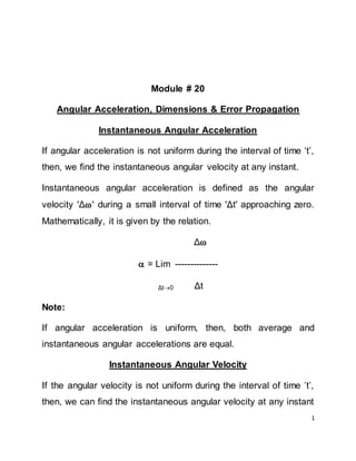
1. 1
Module # 20
Angular Acceleration, Dimensions & Error Propagation
Instantaneous Angular Acceleration
If angular acceleration is not uniform during the interval of time ‘t’,
then, we find the instantaneous angular velocity at any instant.
Instantaneous angular acceleration is defined as the angular
velocity 'Δ' during a small interval of time 'Δt' approaching zero.
Mathematically, it is given by the relation.
Δ
 = Lim --------------
Δt0 Δt
Note:
If angular acceleration is uniform, then, both average and
instantaneous angular accelerations are equal.
Instantaneous Angular Velocity
If the angular velocity is not uniform during the interval of time ’t’,
then, we can find the instantaneous angular velocity at any instant

2. 2
which is defined as the angular displacement in a very small
interval of time.
OR
The angular velocity at a particular instant is called instantaneous
angular velocity.
Average Angular Acceleration
If 'i' is the initial angular velocity of a rotating body (like a disc or
wheel etc.) and 'f’ is its final angular velocity after an interval of
time 'Δt', then, the magnitude of average angular acceleration 
is given by;
f -i
 = ------------
Δt
If, f - i =Δ (change in angular velocity)
Then the magnitude of  can be written as;
Δ
 = ------------
Δt

3. 3
Average Angular Velocity
The average angular displacement per second is called average
angular velocity. It is dented by .
Thus,
Average angular displacement ()
Average Angular Velocity =  = -------------------------------------------
Time
Angular Acceleration
The angular acceleration is defined as the rate of change of
angular velocity. It is denoted by '' (alpha).
Change in angular velocity
Angular acceleration = ---------------------------------------
time
Let 'Δ' be the change of angular velocity in a time interval 'Δt',
then

4. 4
Δ
 = ---------
Δt
Units of Angular Acceleration
The SI units of angular acceleration are radian per second per
second or written as rad s-2
.
Other Units are revolution per second per second or written as
revs-2
and degrees per second per second or written as degs-2
.
Direction of Angular Acceleration ()
Angular acceleration is a vector quantity. Like a linear
acceleration, angular acceleration can also have positive or
negative value. When the angular acceleration is positive, then,
the body rotates faster and when it is negative, then, the body
tends to be slower.
If the direction of rotation does not change, then, the direction of
angular acceleration () is along the axis of rotation. If, however,
angular velocity ‘’ increases, then, '' and '' are parallel to each
other.

5. 5
Centripetal Force or Centre Seeking Force
Centripetal force is the force required to keep a body moving in a
circle and which is directed towards the centre.
mv2
F = ------------------
R
Thus, the centripetal force is that force which compels a body to
move along a circular path and is always directed towards the
centre of the circle.
According to Newton's second law of motion, whenever an object
accelerates, there must be a net force acting on it to produce this
acceleration. Therefore, in a uniform circular motion, there must
be a net force to produce this centripetal acceleration.
For example, in the case of a satellite circling the earth, the
necessary force is supplied by gravity which is directed towards
the centre of the earth. Such a force is called the centripetal force.
In other words, centripetal force is the force that must be applied
to an object towards the centre of a circle to make the object
move round the circle. Without this centripetal force, circular
motion cannot take place.

6. 6
According to Newton's second law of motion, this force produces
an acceleration in its own direction. Therefore, the direction of
force producing centripetal acceleration is the same as that of the
centripetal acceleration.
If m is the mass of the object, then the centripetal force Fc is given
by the equation,
Fc = mac __________ [1]
We know that centripetal acceleration ac is given by,
ac = v2/r___________ [2]
Using [2] in [1], we get,
Fc = mv2
/r
Examples of Centripetal Force
For the importance of centripetal force in circular motion, consider
the following examples.
(1) A ball of mass m is attached to one end of a string. The ball
is whirled by moving the hand (while holding the other end) in a
circle in a horizontal direction as shown in figure (1).
In order to keep the ball in a circle, we have to apply a centripetal
force by pulling the string towards the centre of circle. If we let the

7. 7
string go, the ball moves in a direction at a tangent to the original
circular path, with no centripetal force acting on it.
Fig: (1) Centripetal Force
(2) Consider another example which shows the importance of
centripetal force for the continuation of the circular motion. We
observe that when a car moves along a round track, the force of
friction between the tyres and the road provides the necessary
centripetal force and keeps the car on curved path.
If the tyres are worn out and the road is slippery due to some oil
on its surface, then the friction will be insufficient. As a result, the
car will skid off the road.
Moreover, the outer edge of the curved road is made a little
higher than the inner edge at the corners. This is called banking
of the road, because, while moving along the curve, the car
presses down the road and the reaction on the car acts normal to
the road. The vertical component of the reaction force balances

8. 8
the weight of the car and the horizontal component provides the
necessary centripetal force for the car to take the turn.
(3) The electrostatic force of attraction between positively
charged nucleus and negatively charged electrons provides the
necessary centripetal force for the orbital motion of electrons
around the nucleus in an atom.
Centrifugal Force
Centrifugal force is a reaction force. It is equal to the centripetal
force and acts in opposite direction. Thus centrifugal force tends
to act only as long as the centripetal force is acting. It ceases to
act, the moment, centripetal force vanishes.
We know that centripetal force is necessary to keep a body in its
uniform circular motion. When we whirl a ball at the end of a
string, we transmit this centripetal force to the ball by means of
the string, pulling it inward, and thus keeping it in the circular path.
According to Newton's third law of motion, the ball will react and
will exert an equal and opposite force outward on the hand. This
outward pull force on our hand is called the centrifugal force. It is
a reaction force.
Centripetal Acceleration

9. 9
The acceleration produced by the centripetal force is always
directed towards the centre of a circular path and, therefore, it is
called centripetal acceleration.
Explanation
If a body moves in a circle with constant speed, then, the
magnitude of the velocity remains constant, but, its direction
changes continuously. Due to this change in velocity, the body
must have an acceleration which is directed towards the centre of
the circle. Such an acceleration of the body which is always
directed towards the centre of the circle is known as centripetal
acceleration.
Dimensions of Physical Quantities
In physics, the word dimension represents the physical nature of
a quantity. A distance may be measured in feet or in meters but it
is still a distance. We say, its dimension is length. In the same
way, irrespective of the system of units and the quantities, the
dimension of mass is mass and that of time is time. The symbol L,
M and T are used to specify length, mass and time respectively.
Square brackets [ ] are used to denote the dimension of a
physical quantity. For example, velocity is defined as distance
travelled per unit time. Since, the distance is length, so the
dimensions of velocity in this notation are written as [v] = [L/T] =

10. 10
[LT-1]. The dimensions of area A are [A] = [L2]. The dimensions of
volume V are [V] = [L3
] and those of acceleration are [a] = [L /T2
] =
[LT-2
].
Similarly, the dimensions of force are [F] = [MLT-2
]. The
dimensions of work are [W] = [ML2
T-2
]. The dimensions of weight
are given by MLT-2. [It means Force & Weight have same
dimensions. F= ma & W = mg]. The dimensions of angular
momentum (L) are ML2
T-1
. The dimensions of power are ML2
T-3
.
The dimensions of torque are ML2
T-2
. [It means work & torque
have same dimensions.]. The dimensions of pressure are ML-1
T-2
.
The dimensions of frequency are T-1. The dimensions of linear
momentum are MLT-1
. The dimensions of impulse are MLT-1
. [It
means impulse & linear momentum have same dimensions.] The
dimensions of density are ML-3
. The dimensions of angular
momentum (L) are ML2
T-1
. The dimensions of angular velocity ()
are T-1. The dimensions of Co-efficient of Viscosity () are ML-1T-1.
Uses of Dimensions
(1) To Derive the Equations: The dimensions of various
physical quantities are useful in deriving the equations. Many
equations have been derived in this way.

11. 11
(2) To Test the Correctness of Equations: By substituting the
dimensional formula on both the sides of an equation, any
physical equation can be checked.
Significant Figures
The number of digits about which we are reasonably sure is
called the significant figures.
OR
In any measurement, the accurately known digits and the
first doubtful digit are known as significant figures. Whenever, we
make any measurement, only the number of significant figures
must be used. Additional number of digits must be avoided
otherwise it will mislead the students into believing them as
correct.
In order to clarify the concept of significant figures, let us
analyze the statement that 50,000 people witnessed the military
parade. This statement in no way gives us the information as
regards actual number of persons present. If the observer had
taken thousand as the unit of counting, then, obviously, the
observer counted 500 or more than 500 (501 to 999) persons as
one thousand and ignored those who were less than 500 (1 to
499). The information, therefore, is correct only in thousands i.e.,
fifty thousand but not in hundreds, tens, or units. In this case, only

12. 12
two figures 5 and 0 in 50,000 are significant. In this very case, if
the observer had chosen hundred as a unit of counting and had
recorded the number of persons as 50000 i.e., five hundred
hundreds, then, three figures given in the box were significant.
Similarly, had he chosen ten as his unit of counting, and had
again recorded the number 50000 i.e. five thousand tens, then,
four figures in the box were significant. If he had actually counted
the persons one by one and had recorded the number 50,000,
then, all the five digits would be significant.
Let us try to find the number of significant figures in the
following cases:
5142 All significant
50201 -Do-
50000 Digit 5 is significant count, zeros may or may not
be significant.
0.2020 All digits after the decimal point are significant, but zero
before the decimal point is not significant.
0.1000 All digits after the decimal are significant, but zero
before the decimal point is not significant.
0.0010 Digits 1 and 0 on the right are significant. Zeros on the
left of 1 are not significant. This is due to the fact that the number
is a fraction and may be written as 10x10-4
or 1.0 x 10-3
.

13. 13
0.0001 Only the digit 1 is significant. It is also a fraction and
may be written as 1 x 10-4
.
1.00 x 10-3
Three digits 1 and 0, 0 before 10-3
are significant.
1.0020 All the digits are significant.
General Rules
(1) All the digits 1,2,3,4,5,6,7,8,9 are significant digits. However,
zeros may or may not be significant. In case of zeros, the
following rules may be adopted.
(2) Zeros to the left of a significant digit, not in between two
digits are not significant e.g., 0.000135, 01.56, 0.0632. None of
the zeros is significant.
(3) Zeros to the right of a significant digit may or may not be
significant. In decimal fractions, zeros to the right of a significant
figure are significant e.g. 2.320, 6.2000, 9.30200. However, if the
number is an integer i.e., a whole number such as 50000, the
zeros may or may not be significant (See example of military
parade above).
Precision of Measurement
The closeness of a set of measured values with one another is
called precision. The greatest possible error is considered to be ±

14. 14
half the least division of measurement of an instrument. The
measurements which have less error are called precise.
When one makes some sort of measurement, then, the
measured value is known to be within limits of some experimental
uncertainty (or error). This error or uncertainty may be due to a
faulty instrument or due to carelessness, lack of experience or
training on the part of the observer. The type of instrument used
may as well be responsible for this uncertainty (or error). For
example, while recording a certain thickness with a meter-rod, a
vernier calipers or a screw-gauge, the uncertainty in
measurement would be greater in case of measurement with a
meter rod than the one made with the help of a screw-gauge.
To make this point clearer, one may realize that every instrument
is calibrated to a certain smallest division, which puts a limit to the
degree of precision which may be achieved on making
measurement with it. A reading which may fall within the two
marked divisions can only be guessed (or estimated) and can
therefore be hardly considered as correct. For example, while
measuring length of a straight line with a meter-rod calibrated in
millimeters, if the length is read as 12.43 cm, 12.44 cm, 12.45 cm,
12.46 cm or 12.47 cm, one cannot be sure as regards the figures
at the second decimal point, since these have just been guessed.

15. 15
The least division on a meter rod is 1 mm. or 0.1 cm. Therefore,
maximum possible error is ± half of 0.1 cm that is 0.05 cm. A
general practice in measurement is that if the end of the line
doesn't appear to have touched or crossed the mid-point (or half)
of the smallest division, then, the reading may be confined to the
previous division. In case the end seems to be touching or to
have crossed the mid-point, then, the reading is finalized as
extended to the next division. It is, therefore, logical to assume
that a reading recorded as 12.4 cm with the help of a meter-rod
correct up to a millimeter only may fall between 12.35 cm and
12.45 cm (Please note the word between). The same fact may be
stated by saying that the maximum possible error or guess in this
reading is ±0.05 cm i.e., half of the least division marked on the
meter-rod or the measuring instrument. The correct way of
recording the above reading is:
12.4 ±0.05 cm
Accuracy and Relative Error
Relative error is defined as the ratio of the error to the quantity
measured.
The closeness of the average of measured values and the
accepted (true) values is called accuracy.

16. 16
Consider two measurements viz., 15.4 cm. and 3215 km. The first
measurement may have a maximum error of 0.05 cm (As the
greatest possible error is considered to be ± half the least division
of measurement of an instrument. The least division on a meter
rod is 1 mm. or 0.1 cm. Therefore, maximum possible error is ±
half of 0.1 cm that is 0.05 cm), while the second measurement
may have a maximum error of 0.5 km. An error of 0.05 cm
obviously is smaller than an error of 0.5 km. The first
measurement, having smaller error, is considered to be more
precise than the second one having greater error. However, if we
calculate Relative Error i.e., error divided by the measured
quantity, then, we get the following results for the two cases:
First case:
Error 0.05 cm
Relative Error = --------------------------- = --------------  0.003
Quantity Measured 15.4 cm

17. 17
Second case:
Error 0.5 km
Relative Error = --------------------------- = --------------  0.0002
Quantity Measured 3215 km
The second measurement, though less precise, has smaller
relative error than the first measurement which is more precise.
Therefore, the second measurement though less precise is more
accurate. Hence, precision stands for the magnitude of error in a
measurement, whereas, accuracy stands for relative error. Lesser
is the relative error, more accurate is a measurement.