The high mass_stelar_initial_mass_function_in_m31_clusters

THE HIGH-MASS STELLAR INITIAL MASS FUNCTION IN M31 CLUSTERS*
Daniel R. Weisz1,12
, L. Clifton Johnson1
, Daniel Foreman-Mackey2
, Andrew E. Dolphin3
, Lori C. Beerman1
,
Benjamin F. Williams1
, Julianne J. Dalcanton1
, Hans-Walter Rix4
, David W. Hogg2,4
, Morgan Fouesneau4
,
Benjamin D. Johnson5
, Eric F. Bell6
, Martha L. Boyer7
, Dimitrios Gouliermis4,8
, Puragra Guhathakurta9
,
Jason S. Kalirai7
, Alexia R. Lewis1
, Anil C. Seth10
, and Evan D. Skillman11
1
Astronomy Department, Box 351580, University of Washington, Seattle, WA, USA; dweisz@uw.edu
2
Center for Cosmology and Particle Physics, New York University, 4 Washington Place, New York, NY 10003, USA
3
Raytheon Company, 1151 East Hermans Rd, Tucson, AZ 85756, USA
4
Max Planck Institute for Astronomy, Koenigstuhl 17, D-69117 Heidelberg, Germany
5
Harvard-Smithsonian Center for Astrophysics, 60 Garden Street, Cambridge, MA 02138, USA
6
Department of Astronomy, University of Michigan, 500 Church Street, Ann Arbor, MI 48109, USA
7
Space Telescope Science Institute, 3700 San Martin Drive, Baltimore, MD 21218, USA
8
Universität Heidelberg, Zentrum für Astronomie, Institut für Theoretische Astrophysik, Albert-Ueberle-Str. 2, D-69120 Heidelberg, Germany
9
Department of Astronomy, University of California at Santa Cruz, 1156 High Street, Santa Cruz, CA 95064, USA
10
Department of Physics and Astronomy, University of Utah, Salt Lake City, UT 84112, USA
11
Minnesota Institute for Astrophysics, University of Minnesota, 116 Church Street SE, Minneapolis, MN 55455, USA
Received 2015 February 19; accepted 2015 May 14; published 2015 June 18
ABSTRACT
We have undertaken the largest systematic study of the high-mass stellar initial mass function (IMF) to date using
the optical color–magnitude diagrams (CMDs) of 85 resolved, young ( t4 Myr 25 Myr), intermediate mass
star clusters (103
–104
Me), observed as part of the Panchromatic Hubble Andromeda Treasury program. We fit
each cluster’s CMD to measure its mass function (MF) slope for stars 2 Me. By modeling the ensemble of
clusters, we find the distribution of MF slopes is best described by 1.45 0.06
0.03
with a very small intrinsic
scatter and no drastic outliers. This model allows the MF slope to depend on cluster mass, size, and age, but the
data imply no significant dependencies within this regime of cluster properties. The lack of an age dependence
suggests that the MF slope has not significantly evolved over the first ∼25 Myr and provides direct observational
evidence that the measured MF represents the IMF. Taken together, this analysis—based on an unprecedented
large sample of young clusters, homogeneously constructed CMDs, well-defined selection criteria, and consistent
principled modeling—implies that the high-mass IMF slope in M31 clusters is universal. The IMF has a slope
( 1.45 0.06
0.03
; statistical uncertainties) that is slightly steeper than the canonical Kroupa ( 1.30) and Salpeter
( 1.35) values, and our measurement of it represents a factor of ∼20 improvement in precision over the Kroupa
IMF (+1.30 ± 0.7). Using our inference model on select Milky Way (MW) and LMC high-mass IMF studies from
the literature, we find 1.15 0.1MW and 1.3 0.1LMC , both with intrinsic scatter of ∼0.3–0.4 dex.
Thus, while the high-mass IMF in the Local Group may be universal, systematics in the literature of IMF studies
preclude any definitive conclusions; homogenous investigations of the high-mass IMF in the local universe are
needed to overcome this limitation. Consequently, the present study represents the most robust measurement of the
high-mass IMF slope to date. To facilitate practical use over the full stellar mass spectrum, we have grafted the
M31 high-mass IMF slope onto widely used sub-solar mass Kroupa and Chabrier IMFs. The increased steepness in
the M31 high-mass IMF slope implies that commonly used UV- and Hα-based star formation rates should be
increased by a factor of ∼1.3–1.5 and the number of stars with masses 8 Me is ∼25% fewer than expected for a
Salpeter/Kroupa IMF.
Key words: galaxies: star clusters: general – galaxies: star formation – Hertzsprung–Russell and C–M diagrams –
Local Group – stars: luminosity function, mass function
1. INTRODUCTION
The stellar initial mass function (IMF), for ⩾M 1 Me plays
a central role in a wide variety of astrophysics. The relative
number of such stars is essential to interpreting the stellar
populations of star-forming galaxies across cosmic time, testing
and validating theories of star formation, constraining chemical
evolution models, the formation of compact objects and
gravitational waves, and understanding the interplay between
stars and gas (e.g., Schmidt 1959; Tinsley 1968; Searle et al.
1973; Talbot & Arnett 1973; Ostriker et al. 1974; Audouze &
Tinsley 1976; Scalo 1986; Kennicutt 1998a; Elmegreen 1999;
Kroupa 2001; Massey 2003; Alves et al. 2007; Fardal et al.
2007; McKee & Ostriker 2007; Wilkins et al. 2008; Pflamm-
Altenburg & Kroupa 2009; Kennicutt & Evans 2012;
Narayanan & Davé 2012; Conroy 2013; Kroupa et al. 2013;
Belczynski et al. 2014; Krumholz 2014; Madau & Dick-
inson 2014).
1.1. Current State of the IMF Above ∼1 Me
Our best constraints on the high-mass IMF come from
studies in the Milky Way (MW) and nearby galaxies. For the
closest galaxies, it is possible to count individual stars and
The Astrophysical Journal, 806:198 (13pp), 2015 June 20 doi:10.1088/0004-637X/806/2/198
© 2015. The American Astronomical Society. All rights reserved.
* Based on observations made with the NASA/ESA Hubble Space Telescope,
obtained at the Space Telescope Science Institute, which is operated by the
Association of Universities for Research in Astronomy, Inc., under NASA
contract NAS 5-26555. These observations are associated with program
#12055.
12
Hubble Fellow.
1

make a direct measurement of the high-mass IMF slope. While
measuring the IMF from direct star counts is straightforward in
principle, it is far more complicated in practice. Accurate
measurements are challenging due to a variety of observational
and physical effects including completeness, dynamical evolu-
tion, distance/extinction ambiguity, stellar multiplicity, the
accuracy of stellar evolution models, degeneracies between star
formation history (SFH) and the IMF slope, and a paucity of
massive stars in the nearby universe, all of which complicate
the translation of the present day mass function (MF) into the
IMF (e.g., Lequeux 1979; Miller & Scalo 1979; Scalo 1986;
Mateo et al. 1993; Massey et al. 1995a; de La Fuente Marcos
1997; Maíz Apellániz & Úbeda 2005; Elmegreen & Scalo
2006; Maíz Apellániz 2008; Ascenso et al. 2009; Kruijssen
2009; Bastian et al. 2010; De Marchi et al. 2010; Portegies
Zwart et al. 2010; Kroupa et al. 2013; Schneider et al. 2015).
Observations of more distant, unresolved galaxies alleviate
some of these challenges. For example, by studying an entire
galaxy, effects of stellar dynamics (e.g., migration, mass
segregation) and distance/extinction confusion are less impor-
tant. Further, distant galaxies offer far more diversity than what
is available in the very local universe and provide better
opportunities to explore the high-mass IMF as a function of
environment (metallicity, mass, redshift, etc.; e.g., Baldry &
Glazebrook 2003; Fardal et al. 2007; Davé et al. 2011;
Narayanan & Davé 2013).
However, the unresolved nature of these observations
severely limits the precision and accuracy of any high-mass
IMF measurement. Most integrated observations provide
insufficient leverage to mitigate the SFH-IMF degeneracy,
and we are forced to make simplifying assumptions about a
galaxy’s recent SFH (e.g., constant, single short burst) and dust
(e.g., a single value for an entire galaxy) to provide any
constraint on the high-mass IMF (e.g., Miller & Scalo 1979;
Elmegreen & Scalo 2006). Although studies of unresolved
clusters may provide a new avenue for IMF studies (e.g.,
Calzetti et al. 2010; Andrews et al. 2013; although see Weidner
et al. 2014 for a contrasting perspective), high-mass IMF
studies using integrated light typically provide coarse char-
acterizations rather than precise measurements.
As a result of these challenges, our current knowledge of the
high-mass IMF remains remarkably poor. The widespread
adoption of a “universal” Salpeter ( 1.35; Salpeter
1955) or Kroupa ( 1.3; Kroupa 2001) IMF above
1 Me, presumed not to vary with environment has given the
impression that the high-mass IMF is a solved problem (e.g.,
Kennicutt 1998a). However, compilations of IMF studies in the
literature from resolved star counts indicate an “average value” of
1.7 with a scatter 0.5 dex in IMF slope measurements that
does not clearly support a “universal” IMF (e.g., Scalo 1986,
1998; Kroupa 2002; Scalo 2005).13
There also does not appear to
be any unambiguous systematic dependence of IMF slope on
environment and/or initial star-forming conditions (e.g., Bastian
et al. 2010), which has significant implications for how stars form
in a wide variety of physical conditions (e.g., Elmegreen 1999;
McKee & Ostriker 2007; Hopkins 2013; Krumholz 2014).
Controversy over the form and universality of the IMF have
persisted since the first studies in the 1950s. Following the
seminal work of Salpeter (1955), a handful of studies reported
similar IMFs in a number of MW clusters and field
environments (Jaschek & Jaschek 1957; Sandage 1957; van
den Bergh 1957), prompting early speculation about the
universality of the “original MF” (e.g., Limber 1960; van
den Bergh & Sher 1960). However, this early agreement with
Salpeter gave way to large scatter in IMF measurements
beginning in the 1970s, as several studies with more
sophisticated completeness corrections and updated stellar
physics highlighted the shortcomings in the first generation
of IMF studies (e.g., Taff 1974; Lequeux 1979; Tarrab 1982).
Furthermore, Miller & Scalo (1979) provided a comprehensive
reassessment of the MW field star IMF, in light of the
previously unaccounted for SFH-IMF degeneracy. They
suggested a high-mass IMF of the with 1.5 for stars 1 
M/Me  10 and 2.3 for stars M/Me  10. However,
Kennicutt (1983) showed that such a steep IMF slope above
∼10 Me was incompatible with observations of B V colors
and Hα equivalent widths in nearby disk galaxies, suggesting
that extrapolating the value of 1.5 from 1–100 Me
provided a better match to the data. This conclusion was
further solidified in Kennicutt et al. (1994).
The number of observational high-mass IMF studies peaked
between the late 1980s and early 2000s. This golden age
followed the comprehensive IMF review by Scalo (1986),
which concluded that systematic uncertainties were the
dominant source of confusion in our poor knowledge of the
IMF. Shortly after, the proliferation of CCDs enabled
significant progress in reducing these systematics, primarily
by allowing for quantitative completeness corrections via
artificial star tests (ASTs; e.g., Stetson 1987; Mateo et al.
1993). The 1990s saw a flurry of qualitatively new IMF studies
including star counts in the LMC, spectroscopy of starburst
galaxies, and IMF constraints from stellar abundance patterns
(see Leitherer 1998; Massey 1998; Gilmore 2001 for extensive
discussion of the literature in these areas). The sheer number
and richness of IMF studies from this era precludes a detailed
history in this paper, and we instead refer readers to a number
of excellent papers that chronicle the history of the IMF (e.g.,
Scalo 1986, 2005; Massey 1998, 2003; Kennicutt 1998a;
Elmegreen 1999, 2006; Eisenhauer 2001; Gilmore 2001;
Zinnecker 2005; Bastian et al. 2010; Kroupa et al. 2013).
To briefly summarize, many studies from this era concluded
that the high-mass IMF in the local universe was not drastically
different from Salpeter over a wide range of environments
(e.g., Leitherer 1998; Massey 1998, 2003; Gilmore 2001;
Kroupa 2001). However, there was no clear explanation for the
observed scatter in the measured IMF slopes, which contradicts
a truly universal high-mass IMF. Some have argued that
measurement uncertainty and systematics are the dominant
source of scatter (e.g., Elmegreen 1999; Kroupa 2001, 2002;
Massey 2003). However, without systematically revisiting each
study, it is challenging to dismiss the scatter as solely a
measurement uncertainty. As a clear counterexample, there are
well-known studies of star clusters with some of the same
physical properties (e.g., age, mass) that have been analyzed
identically, but have very different high-mass IMF slopes (e.g.,
Phelps & Janes 1993), reinforcing that some of the scatter may
be physical in nature. In a broader analysis of the literature,
(Weisz et al. 2013) show that >75% of published resolved star
IMF studies significantly underreport uncertainties relative to
the theoretically possible precision, which underlines the
13
Although a “Kroupa IMF” has a high-mass slope of 1.3, Kroupa
(2002) argue that the slope should probably be close 1.7, as most
historical IMF studies do not account for unresolved binary stars, which, in
principle, cause measured MF slopes to be shallower than true IMF slopes.
2
The Astrophysical Journal, 806:198 (13pp), 2015 June 20 Weisz et al.

difficulty in disentangling systematics from intrinsic IMF
variation using IMF studies in the literature.
Since the early 2000s, studies of the high-mass IMF have
diminished in number, as attention turned to the sub-solar regime
(e.g., Chabrier 2003; Scalo 2005; Zinnecker 2005). However,
focus on the high-mass IMF was recently rekindled following
several reports of a systematic deficit of massive stars in lower-
luminosity galaxies, based on observations of integrated broad-
band and/or Hα-to-UV flux ratios (e.g., Hoversten & Glazebrook
2008; Boselli et al. 2009; Lee et al. 2009; Meurer et al. 2009).
Yet, whether these observations are indicative of a systematically
varying IMF (e.g., Weidner & Kroupa 2005; Pflamm-Altenburg
& Kroupa 2009; Kroupa et al. 2013) remains an open question,
as other mechanisms such as stochastic sampling of the cluster
MF and/or bursty SFHs can also explain these observed
properties (e.g., Fumagalli et al. 2011; da Silva et al. 2012;
Weisz et al. 2012). Other recent studies have challenged the
universality of the high-mass IMF (e.g., Dib 2014), but broader
conclusions are limited by the small sample sizes.
After decades of study, the most commonly used high-mass
IMF is a universal Salpeter/Kroupa IMF that is perfectly known
(i.e., uncertainties are typically not included). However, this de
facto standard IMF is not unambiguously supported by a large
number of literature IMF studies. This tension is the direct
result of a continued reliance on a rich, but heterogenous set of
literature IMF studies, and can only be resolved through a
large, homogenous survey of individually resolved young,
massive stars.
1.2. The IMF > 2–3 Me in M31
A primary goal of the Panchromatic Hubble Andromeda
Treasury program (PHAT; Dalcanton et al. 2012) is a
comprehensive exploration of the stellar IMF above ∼2–3 Me.
This 828-orbit Hubble Space Telescope (HST) multi-cycle
program acquired near-UV through the near-IR imaging of
∼120 million resolved stars in ∼1/3 of M31ʼs star-forming disk
(Williams et al. 2014), providing a dataset of unprecedented
size and homogeneity for measuring the high-mass IMF.
The focus of the present IMF study is on M31ʼs young star
cluster population. Star clusters provide a more direct path to
measuring the IMF compared to field populations, which suffer
from IMF-SFH degeneracies for stars more luminous than the
oldest main sequence turnoff (e.g., Miller & Scalo 1979;
Elmegreen & Scalo 2006); furthermore, the differential
extinction found in the disk of M31 (e.g., Draine et al. 2013;
J. J. Dalcanton 2015, in preparation), and similarly sized star-
forming galaxies, adds a significant layer of complexity to
modeling the field stellar populations (e.g., Lewis et al. 2015).
In contrast, star clusters provide a relatively simple way to
probe the IMF. Their coeval nature genuinely mitigates the
effects of SFH, while their vulnerability to foreground
differential extinction is minimal due to their small sizes.
In this paper, we focus on determining the MF slopes for
PHAT clusters that are 25 Myr old and 103
Me in mass
using resolved star color–magnitude diagrams (CMDs). For
these clusters, the detectable portion of the main sequence is
well-populated from ∼2 Me to 25 Me
14
and they are of order
∼0.1 relaxation times old, which mitigates the strongest effects
of mass segregation, making them an ideal sample with which
to study the high-mass IMF. We model the optical CMD of
each cluster k to constrain its power-law slope k of the present
day high-mass MF, p( )k , marginalized over other parameters
of that fit (e.g., cluster age, extinction, binarity).
Subsequently, we propose a simple model for the ensemble
properties of the cluster MF, with a mean, Γ, and a scatter, ,
and fit it to the MF probability distribution functions (PDFs) of
the individual clusters. We also use this model to search for
possible dependencies of Γ on cluster mass, age, and size. We
verify this approach with an extensive set of artificial clusters
that were inserted into PHAT images, processed, and analyzed
identically to the real clusters.
This paper is organized as follows. In Section 2, we define
our cluster sample and briefly describe the PHAT photometry,
ASTs, and artificial cluster sample. We outline our method of
modeling the cluster CMDs in Section 3 and present the results
for the ensembles of real and artificial clusters in Section 4.
Finally, in Section 5, we discuss our findings in the context of
current and historical views on the high-mass IMF and
illustrate the implications of our results.
2. DATA
2.1. Cluster Sample
Clusters in PHAT were identified as part of the Andromeda
Project,15
a collaborative effort between PHAT and the
Zooniverse16
citizen science platform. As described in Johnson
et al. (2015), cluster candidates were assigned probabilities of
actually being a cluster based on citizen scientist ranking.
These probabilities were verified using synthetic cluster results
and comparison with the preliminary catalog, which was
assembled by professional astronomers (Johnson et al. 2012).
Extensive details of the cluster identification methodology can
be found in Johnson et al. (2015).
For the present study, we have limited our analysis to the 85
clusters with CMD-based ages 25 Myr and masses 103
Me (L. C. Beerman 2015, in preparation), and half-light radii
2 pc (Johnson et al. 2015). We focus on these young, more
massive clusters in PHAT to avoid the very sparse sampling in
the low-mass clusters; to limit the impact of stellar crowding in
the densest clusters; to facilitate the extrapolation of the
observable MF to an IMF; and to remain in the regime of high
completeness (>90% for our sample; see Figure 10 in Johnson
et al. 2015). We will explore each of these issues in detail in
our comprehensive study of PHAT cluster MFs in a future
paper.
2.2. Cluster Photometry
Photometry of PHAT clusters was performed using DOL-
PHOT,17
a version of HSTPHOT (Dolphin 2000) with HST
specific modules, following the description in Williams et al.
(2014).18
For reasons discussed below, we made slight changes
to the survey-wide photometry in that we re-reduced the entire
survey using only the optical images (F475W, similar to SDSS
g; and F814W, similar to I-band). The optical image and CMD
14
Accurately inferring the masses of stars above ∼25 Me requires optical
spectroscopy (e.g., Massey et al. 1995a); thus from the PHAT optical
photometry we can only estimate a lower-limit for masses of the most luminous
stars.
15
http://www.andromedaproject.org
16
https://www.zooniverse.org
17
http://americano.dolphinsim.com
18
http://archive.stsci.edu/missions/hlsp/phat/
3

of a typical cluster used in this study are shown in Figures 1
and 2.
For the purposes of this paper, we only use optical
photometry, which contains the most information about the
IMF slope, particularly when modulated by observational and
computational considerations. In principle, the full spectral
energy distribution (SED) of each star can increase the degree
of precision to which we know its mass, and, in turn provide
improved constraints on the IMF. However, the UV and IR
photometry in PHAT clusters typically contains fewer than
∼50% the number of stars detected in the optical, reducing their
statistical utility for constraining the MF slope (see Weisz et al.
2013). PHAT UV imaging is significantly shallower (∼2 mag)
than the optical, even along the main sequence, resulting in
many fewer sources detected. The IR also yields far fewer main
sequence stars as a result of significant crowding due to the
lower angular resolution of the WFC3/IR camera.
There are also subtle systematics associated with non-optical
bands. For example, the UV and IR bolometric corrections are
not as certain as those in the optical, particularly for massive,
metal-rich stars, which can introduce systematics into our
analysis.
Finally, the modest gain (at best) in precision in the MF
slope of each cluster must be balanced against the computa-
tional cost of processing >10 million additional ASTs. Thus, by
only reducing and analyzing the optical data, we retain virtually
all statistical leverage on measuring the MF slope, but save
considerably on computational costs.
However, analysis of the full stellar SEDs is valuable for
searching for the most massive stars in clusters. In addition to
the slope, the maximum stellar mass plays a fundamental role
in defining the high-mass IMF, but is unconstrained by the
approach we use to measure the MF slope (e.g., Weisz et al.
2013). An investigation of the most massive stars in the PHAT
area is the subject on an ongoing study and will be presented in
a future paper.
For each cluster, we ran ∼50,000 ASTs by adding stars of
known luminosities one at a time (to avoid artificially
enhancing crowding effects) into the PHAT optical images of
each cluster. The input ASTs were uniformly distributed over
each cluster’s CMD and spatially distributed approximately
according to each cluster’s light profile. Extensive testing
showed that such a spatial scheme was necessary to accurately
characterize the completeness and photometric uncertainty
profiles of the clusters, as a simple uniform spatial scheme
results in overly optimistic completeness and photometric
uncertainty profiles. Similarly, our adoption of a uniform
distribution of ASTs in CMD space (as opposed to only
matching a given cluster’s CMD) is necessary to evaluate all
possible cluster models (i.e., all combinations of age, mass,
metallicity, membership, IMF). In contrast, only using ASTs
that roughly follow a cluster’s observed CMD would result in a
poor noise model for less obvious possible combinations of
cluster properties (e.g., stochastic sampling of the IMF can be
degenerate with cluster age), inhibiting a comprehensive search
of likelihood space. Finally, we tested the effects of the number
of ASTs (ranging from 10,000 to >100,000) used on the
recovery of cluster parameters. We found that 50,000 ASTs
provided an optimal balance between stability of the solutions
and computational efficiency.
2.3. Artificial Clusters
We use extensive sets of artificial clusters to verify the
accuracy of each component of our MF determinations,
including photometry, ASTs, and CMD modeling. The
artificial clusters were designed to match the physical proper-
ties of our real cluster sample and span a range of physical
parameters (age, mass, size, extinction) that encompass the real
clusters. The artificial clusters were inserted into images at a
range of galactocentric radii and environments to capture the
full range of background densities in PHAT. Overall, the
artificial cluster tests confirmed that we can accurately recover
Figure 1. HST/ACS optical color image of AP 94, a typical cluster analyzed in
this paper. The angular high-resolution of HST allows us to resolve the
individual stars clusters at the distance of M31. For reference, the image is
∼60 pc on each side.
Figure 2. Panel (a): the optical CMD of AP 94. The gray points are below the
nominal completeness limit, and were not included in the CMD analysis. For
reference, we indicate the main sequence turn-off masses on the left-hand side
and over-plot the best fitting isochrone for this cluster (see Section 3.1 and
Figure 3). Panel (b): the background CMD constructed by selecting all stars in
an annulus surrounding the cluster that has 10x times the cluster area. The
black points in this CMD are used to statistically model background
contribution to the cluster CMD.
4

the true MF from clusters in PHAT imaging, along with all
other cluster physical properties.
3. METHODOLOGY
3.1. Measuring the Stellar Mass Function of a Cluster
To measure the MF of a cluster we construct synthetic
models of its optical CMD using MATCH, a CMD fitting
program described in Dolphin (2002). Briefly, for a given
stellar evolution library, binary fraction, IMF, age, metallicity,
extinction, and distance, MATCH constructs a simple stellar
population (SSP) in the desired filter combinations. This
synthetic SSP is then convolved with completeness and
photometric biases and uncertainties as determined by the
ASTs. The resulting synthetic CMD is then linearly combined
with a suitable CMD of foreground/background populations,
with the relative contribution of each controlled by a scale
parameter. For a given set of these parameters, the synthetic
Hess diagram, the binned number density of stars in the CMD,
is compared to the observed CMD using a Poisson likelihood
function, which is necessary to account for the effects of sparse
sampling. The procedure is repeated over a large grid of
parameters in order to map all likelihood space. For this
analysis, we adopted the Padova stellar evolution models
(Girardi et al. 2002, 2010; Marigo et al. 2008) and we have
listed the other model parameters and their ranges in Table 1.
Of these parameters, we limited the metallicity to a fairly
small range near Z . This was done because (a) the cluster
CMDs are too sparsely populated to provide robust metallicity
constraints and (b) the current metallicity of M31ʼs disk is
known to be approximately solar, with a very weak gradient
based on H II region and supergiant abundances (e.g., Venn
et al. 2000; Trundle et al. 2002; Sanders et al. 2012; Zurita &
Bresolin 2012).
Similarly, we adopted a fixed binary fraction of 0.35, where
the mass ratio of the stars is drawn from a uniform distribution.
Historically, stellar multiplicity has been problematic for high-
mass IMF determinations from luminosity functions (e.g., Maíz
Apellániz & Úbeda 2005; Maíz Apellániz 2008). However, for
CMD analysis, it is much less of an issue for two reasons. First,
the addition of color information provides clear separation
between the single and binary star sequences, minimizing
confusion between the two. In contrast, when only luminosity
information is available, the binary fraction and IMF slope are
essentially degenerate parameters. Second, stellar multiplicity
is observationally less important for high-mass stars compared
to sub-solar mass stars (e.g., Weidner et al. 2009). For stars
above 1 Me, the majority of companion stars are likely to be
significantly less massive and less luminous than the primary
(see Kobulnicky et al. 2014), resulting in minimal change to
the CMDs. Recent work on binary mass transfer suggests that
the precise details of interactions between binary (and multiple)
companions may influence IMF determinations (e.g., de Mink
et al. 2014; Schneider et al. 2015), but full stellar evolution
models that include binary mass transfer are not yet available.
Within PHAT, we verified that our choice in binary fraction
does not change the results. For example, in the case of AP 94
(Figures 2 and 3), we modeled the CMD with binary fractions
of 0.35 and 0.70 and found differences in the resulting IMF
slope constraints to be <0.02 dex. Tests including different
binary fractions on artificial clusters yielded similarly small
changes.
However, we did find that extreme binary fraction values,
i.e., near 0 or 1, resulted in significantly worse CMD fits. In
these two cases, the model either entirely populated the single
star sequence (binary fraction = 0) or only sparsely populated
it (binary fraction = 1), which substantially reduced the
resemblance of the model to the observed CMD. Thus, for the
present work, we adopted a fixed binary fraction of 0.35, which
appears to be a reasonable value from LMC cluster studies
(e.g., Elson et al. 1998).
To model background populations, we construct an
empirical CMD from an annulus around the cluster that is
ten times its size. The large area is necessary to accurately
constrain the background scaling parameter.
Given a set of cluster model parameters (age, extinction,
metallicity, and MF slope) the resulting model CMD, and the
empirically derived CMD for fore-/background sources are
compared to the observed CMD in a likelihood sense (Dolphin
2002). The resulting posterior probabilities, p t A( , , )V are
illustrated in Figure 3 for a typical cluster in the sample. The
prior on metallicity tightly brackets solar metallicity and the
cluster mass emerges as a normalization factor, rather than a fit
parameter. The smoothness of the p t A( , , )V of each cluster
allows us to interpolate in order to increase the resolution of
our PDFs.
Finally, we emphasize that our analysis does not account for
all sources of systematic uncertainty. Perhaps the more
important systematic is the assumed stellar evolution models.
Different stellar models are known to produce CMDs that can
look quite different (e.g., Gallart et al. 2005), particularly for
evolved phases of evolution. In principle, measuring each
cluster’s MF should be done with multiple stellar models, to
assess the robustness of the MF to stellar evolution effects. In
practice, this is currently not possible. Aside from the Padova
models, at this time, there are no other stellar libraries that
Table 1
Parameters for Measuring the MF of an M31 Star Cluster
Parameter Range Grid Resolution Notes
(1) (2) (3) (4)
Γ (−1.2, 5) 0.2 dex MF slope for stars 2 Me
Binary Fraction 0.35 Fraction of Stars with a Companion
Log(Age) (6.60, 9.0) 0.1 dex Cluster Age
AV (0.0, 3.0) 0.05 dex Line of Sight Extinction
(m−M)0 24.47 Adopted Distance Modulus to M31
log(Z) (−0.2, 0.1) 0.1 dex Metallicity
Note. Parameters and their ranges used for modeling M31 cluster CMDs. The adopted distance modulus is from the tip of the red giant branch measurement made by
McConnachie et al. (2005).
5

include the range of ages and phases of stellar evolution
necessary to analyze this diverse cluster population. If such
models become available in the future, we will revisit our
analysis to assess the impact of systematics. In addition to
stellar models, other sources of systematics include the binary
star model (discussed above), the (unlikely) possibility of
significant differential extinction internal to each cluster, the
assumption that the IMF is a power-law over this mass range
(c.f. Scalo 1986 for discussion of various possible forms for the
high-mass IMF), and complex dynamical effects which may
result in the preferential ejection of stars of a particular mass
(e.g., Oh et al. 2015a).
3.2. Inferring the Intrinsic Distribution of Mass Function
Slopes from a Set of Clusters
One challenge for past MF studies was how to combine
measurements from individual clusters into a broader statement
about the MF slope of “clusters in general.” Typically, the
variance weighted mean is used to compute the “average” MF
from an ensemble (e.g., Scalo 1986). However, this can
potentially be a biased estimator (e.g., assumptions of normally
distributed uncertainties), and does not necessarily use all
available information (e.g., the probability that an object is
actually a cluster).
Here, we adopt a framework that allows us to infer
population wide characteristics about the distribution of MF
slopes, given a set of noisy measurements. This model follows
the approach and implementation laid out in Hogg et al. (2010)
and Foreman-Mackey et al. (2014). We briefly describe the
model below and we refer the reader to those papers for more
detail.
As a simple model for the distribution of cluster MFs, we
assume that it can be described by a normal distribution,
 ( , ), with a mean of Γ and an intrinsic dispersion of .
We initially assume that their parameters are independent of
age, mass, and size of the cluster. If we assume the probability
that each object is a cluster, Qk, we can then write down a
Gaussian mixture model likelihood function for the MF of
clusters, where we simply assume that the MFs of falsely
presumed clusters have a different  ( , )false ,false . This
mixture model mitigates the impact of erroneously identified
clusters, without forcing a binary decision on which clusters
have been identified with sufficient confidence.
More explicitly, the mixture model can be written as
( )
( )
( )
( )
( )
( )
( )
( )
Q Q
Q
p , exp 2
1 exp 2 (1)
k k k k
k k
2
false false
2
where k is the marginalized PDF for the MF of the kth object
and Qk is the probability that the kth object is a cluster. Γ and
2
are the mean and variance of the Gaussian of interest for the
clusters and false and false
2
are nuisance parameters for possible
contaminating sources. Simply put, with this model, the more
probable an object is a cluster the more it contributes to the MF
parameters of interest. In this model context, a universal
Kroupa MF would be represented by 1.30 and 02
,
and universal Salpeter MF by 1.35 and 02
.
This same framework also readily allows us to explore
whether the mean MF slope depends on any of the other cluster
properties such as age, mass, and size. Specifically, we can
generalize the model to
( )t M r a
M
M
a
t
t
a
r
r
, , log log log ,
(2)
k k k m
k
t
k
r
k
c c c
where t M r{ , , }k k k are the most likely age, mass, and size for
the kth object and t M r{ , , }c c c are the mean of our cluster
sample in each case. We assume priors that are flat in
a a a, log , , ,m t r over the ranges indicated in Table 1,
and sample these parameters’ PDFs with the affine invariant
ensemble Markov chain Monte Carlo program emcee (Fore-
man-Mackey et al. 2013).19
4. RESULTS
The analysis laid out in Section 3 proceeds in two steps, the
first leading to the MF slope measurements for individual
clusters, p( )k , the second to the characterization of the
intrinsic, i.e., error corrected, distribution of MF slopes in M31
clusters.
The result of the first step, the marginalized PDF, p( )k , for
all 85 sample clusters is illustrated in Figure 4, showing the MF
slope and its uncertainty for each cluster versus its mass. Points
in the top panel are color-coded by age and those in the bottom
panels by their probability of being a cluster. In both cases, the
point size is proportional to the cluster’s half-light radius.
Clusters with larger half-light radii have lower crowding and
thus more accurate MF determination. From a physical
standpoint, the size of a cluster may also reflect the
environmental conditions in which it was born.
While we have used a different methodology here than
Weisz et al. (2013), the error bars on the MF are similar in the
two approaches, limited in both cases by the number of well-
detected cluster members and by the range of stellar masses
they span. For example, consider AP 94, whose CMD and
Figure 3. Joint and marginalized distributions of age, MF slope, and extinction
for a single young M31 cluster, AP 94, that resulted from modeling the
cluster’s optical CMD, which is shown in Figure 2. The dark points in each
panel reflect the regions of high probability and the pixel sizes reflect the grid
resolution as indicated in Table 1. We use the marginalized distribution for Γ
(shaded histogram) in the subsequent modeling of the distribution of MF
slopes (Section 3.2).
19
https://github.com/dfm/emcee
6

derived physical property PDFs are shown in Figures 2 and 3.
Effectively, there are ∼120 stars (after background correction)
between ∼3 and 15 Me on the upper MS that are used for MF
determination. Given these numbers, from Figure 7 in Weisz
et al. (2013), we expect a theoretical uncertainty of 0.3 on
its MF slope. In comparison, the 1-σ uncertainty from the
marginalized MF PDF in Figure 3 is ±0.32, which is very close
to theoretical expectation. Uncertainties in cluster membership,
the exact mass range on the main sequence, etc., can explain
the small difference in these two values. In general, the cluster
MF slopes are generally less precise for older and lower mass
clusters, and follow the expected precision relationship derived
in Weisz et al. (2013).
Figure 4 also gives a qualitative impression of the ensemble
properties of MF measurements. The majority of clusters have
MF slopes that are near the Kroupa (1.30) or Salpeter (1.35)
slopes; 70% of the clusters MF slopes are within ∼1-σ of
Kroupa and ∼92% are within 2-σ. Remarkably, in this large
sample of young clusters we find that none have extremely
steep or flat MF slopes. At least for the parameter space
covered by our cluster sample, extreme MF slope outliers
( 3 ) are quite rare.
The plots also show the lack of strong correlations between
cluster MF slope and their physical properties. From visual
inspection, it is clear that the MF slopes do not show significant
trends as a function of age, mass, size, or probability of being a
cluster. We list the MF slopes for all clusters in the Appendix.
These impressions from Figure 4 are quantified in the second
step of our analysis, where we propose and constrain a simple
model for the cluster’s distribution of MFs (see Section 3.2),
and constrain its parameters through the comparison with all 85
p( )k .
Figure 5 illustrates the result for the five parameters in our
model: the mean MF slope, Γ, and its intrinsic dispersion ,
and the three coefficients that represent linear trends between
the MF slope and cluster age, mass, and size. This plot shows
that the mean MF slope ( 1.46 0.07
0.04
) is steeper than a
Kroupa IMF, that the scatter ( 0.03 0.00
0.1
) is consistent with
expectations from a universal IMF as determined by similar
analysis of the artificial clusters, and that there are no
significant trends between MF slope and cluster physical
properties.
The small degree of scatter is particularly interesting, giving
the visual impression of large variation between single clusters
Figure 4. The typical cluster has an uncertainty on its MF slope
of ∼0.5 dex, but that ensemble scatter scales roughly as
N1 ( )clusters , indicating that a large and homogenous sample
of clusters are needed to statistically identify a universal IMF.
Finally, the limit on at implies that there is no evidence that the
MF slope changes between 4 and 25 Myr. We list summary
statistics for each distribution in Table 2 along with the same
statistics for our analysis of the population of artificial clusters.
Figure 4. Eighty five young, intermediate mass clusters from PHAT used to
measure the high-mass IMF in M31. Both panels show the median of the
probability distribution for for each cluster’s MF slope vs. cluster mass. Points
in the top panel are color-coded by their age, while those in the bottom panel
are color-coded by the probability of being a cluster. In all cases, point sizes are
proportional to half-light radius and the uncertainties in Γ reflect the 68%
confidence interval on the MF slope. The MF slope of each cluster is listed in
the Appendix.
Figure 5. Joint and marginalized distributions for the distribution of cluster
MFs described by Equations (1) and (2). In all panels, except for , the
dashed blue lines represent the 16th, 50th, and 84th percentiles of each
marginalized distribution. The distribution for is highly non-Gaussian,
making the median a poor point estimate. Instead, we use the mode as a point
estimate, as it reflects the most probable portion of the PDF, and use the 68th
percentile to represent an upper limit. For reference, the solid red lines indicate
the value of a Kroupa IMF slope in the panels, the upper uncertainty on
for a universal IMF as determined by similar analysis of artificial clusters, and a
value of zero in the remaining panels. This plot shows that the mean IMF slope
in M31 clusters is steeper than Kroupa, that the recovered scatter is consistent
with expectations of a universal IMF, with a small tail to larger values, and that
there are no significant trends between the IMF slope and age, mass, or size of
the clusters.
7

There are two reasons why the artificial clusters results are
not an exact delta function. First, the finite grid resolution in
p( )k sets a floor of 0.03; second, as is a positive
definite quantity, its most likely estimate from noisy data must
be significantly positive. However, this effect is quite small, as
the lower limit on the scatter for the artificial clusters is
consistent with the minimum possible value, given the
resolution of our individual cluster PDFs.
Given that the scatter is consistent with expectations for a
universal IMF, we can consider a model in which all the
clusters have the same underlying MF i.e., 0. We find an
ensemble-wide value of 1.45 0.05
0.03
, which is consistent with
results from the hierarchical model. For comparison, the same
analysis applied to the artificial clusters yields a value of
1.30 0.04
0.04
. Uncertainties on the two mean values begin to
overlap at the ∼2-σ level. We plot the results of the “universal”
MF model in Figure 6, and adopt this as the measured high-
mass IMF slope of M31 for the remainder of this paper. As
discussed in Section 3.1, the quoted uncertainties are only
statistical in nature.
5. DISCUSSION
The quality of the PHAT data has enabled important
progress on three issues: (1) quantifying the extent to which
an MF measurement reflects an initial MF (IMF) estimate; (2)
accurately determining what the mean IMF slope is in typical
solar-metallicity (cluster) populations of a large disk galaxy;
and (3) assessing the extent to which the IMF is “universal,” in
the sense that it shows very little scatter in the slope, and no
trends of the slope with cluster properties. The fundamental
conceptual limitation of the present approach is that it only
applies to clusters that remain grouped for longer than 4 Myr,
i.e., they have not (yet) disrupted. Our conclusions are based
on measurements of the high-mass IMF that combine a
principled and systematic constraint of each cluster’s MF
slope, from CMD analysis, with a probabilistic modeling
framework to analyze the distribution of MF slopes.
Overall, we find that the high-mass IMF for clusters in M31
is consistent with a universal IMF. That is, as discussed in
Section 4 and illustrated in Figures 5 and 6, the favored high-
mass IMF model has a steeper mean slope than Salpeter/
Kroupa with a small scatter that is inline with expectations for a
universal IMF. Importantly, we also show that the mean MF
slope in clusters of different ages changes by 0.1 per
decade of age. This suggests that the MF slope is unchanged
over the first ∼25 Myrs, and provides direct observational
evidence that the measured MF represents the IMF. In this
sense, our result represents an important reference point for
understanding the potential evolution of the cluster MF with
cluster physical parameters (age, mass, size) and local star-
forming conditions, both of which will be explored in D. R.
Weisz (2015, in preparation).
Of these results, the most robust determination is the mean
IMF slope. Even if we assume that all of the clusters come from
the same underlying IMF (i.e., no scatter) the steep slope
remains. The lack of correlations between mean IMF slope and
cluster physical properties suggests that other potential sources
of bias (e.g., mass segregation) contribute at a negligible level
to our measurement of the mean.
In contrast, it is more challenging to interpret the significance
of the upper bound on the scatter. The results of our inference
suggest that a universal IMF is most probable. However, there
is a tail to the distribution that extends to 0.1 dex, which
exceeds the tail of the same distribution for the artificial
clusters. We believe that this scatter is likely due to sources of
uncertainty not included in our modeling that may artificially
enhance the scatter relative to expectations from the artificial
clusters. For example, mismatches between the stellar models
and real stars are not captured by the artificial cluster tests.
However, the degree to which model-data mismatches
contribute to the scatter is hard to quantify.
Differential effects may also contribute to the observed
scatter. For example, significant cluster-to-cluster variations in
mass segregation or binarity could contribute to the scatter in
ways not captured by the artificial clusters or our model.
Similarly, we impose a single binary fraction for all masses,
which may not be accurate, given that the most massive stars
may be more likely to have equal mass companions than
intermediate mass stars (e.g., Sana et al. 2013; Kobulnicky
et al. 2014). Furthermore, dynamical effects and ejections may
be coupled to the stellar binarity of a given cluster, which could
Table 2
IMF Parameters for Ensemble of Clusters
Parameter Artificial Real Real
Clusters Clusters Clusters
(1) (2) (3) (4)
1 1.29 0.04
0.05
1.46 0.07
0.04
1.45 0.06
0.03
1 0.03 0.00
0.02
0.03 0.00
0.1
L
am 0.01 0.08
0.08
0.05 0.10
0.10
L
at 0.05 0.08
0.07
0.06 0.09
0.12
L
ar 0.02 0.12
0.10
0.05 0.11
0.09
L
Note. Column (2) values of the five parameter model for the ensemble IMF
from Equations (1) and (2). In the case of , we quote the mode of its
marginalized PDF, along with the upper 68% confidence interval, as the
distribution is highly non-Gaussian. Column (3) value of the IMF slope by
fixing all other parameters to zero, i.e., the assumption that the IMF is
“universal.” The listed values reflect the median and surrounding 68%
confidence interval.
Figure 6. Comparison between the expected IMF slope, Γ, from artificial
clusters inserted into PHAT images (blue) and the real clusters (red), under the
assumption that the underlying IMF slope is universal, i.e., 0. The solid
lines indicate the most probable values, while the shaded regions are the 68%
confidence intervals. The uncertainties on the two measurements begin to
overlap at a 2-σ level.
8

also introduce scatter into the measure MFs (e.g., Banerjee &
Kroupa 2012; Oh et al. 2015b). At the same time, given the
modest size of the upper bound, we expect these effects are, at
most, fairly small.
Overall, it is remarkable that the IMF slope is consistent with
the universal in this mass, metallicity, and cluster density
regime. As summarized in Kennicutt (1998a), quantifying the
degree of scatter is one of the most critical aspects of
understanding the IMF, and ultimately how stars form out of
dense gas. The intrinsic scatter we find suggests that individual
clusters should only minimally deviate from the fiducial value,
and that extreme outliers (e.g., 3 ) are quite rare. The
identification of such objects may represent insight into a mode
of star-formation that truly differs from what we observe in this
regime.
5.1. Comparison with Other High-mass IMF Slopes in the
Local Group (LG)
It is important to place our results into context with other
high-mass IMF studies in the LG. Among the strongest
evidence for the universality of the high-mass IMF in the LG
comes from a series of papers that combine spectroscopy and
photometry of resolved, massive stars in clusters and OB
associations in the LMC and MW (Massey et al. 1995a, 1995b;
Massey 1998, 2003).
To summarize, these studies found (a) no drastic differences
between the IMF slopes of very young, <5 Myr star-forming
regions in the MW and LMC, despite large differences in
metallicity; and (b) that the resulting IMF slopes are broadly
consistent with Salpeter/Kroupa. Combined, these studies
represented a major milestone in our understanding of the
high-mass IMF and its (in-)sensitivity to environment.
Although re-analyzing these studies is beyond the scope of
this paper, we can quantify what the ensemble high-mass IMF
slopes are in the LMC and MW using data from Massey
(2003). The purpose is to give a general sense of how different
our M31 result is from other LG environments. To perform this
analysis, we extracted the necessary data from Massey (2003)
and have listed it in Table 3. We simply use the model from
Equation (1) with Q 1k for each object, i.e., we know they
are all bone fide clusters, to infer the mean and variance for the
MW and LMC clusters. We do not model possible age, mass,
size dependencies.
From this exercise we find mean values of 1.16MW 0.10
0.12
and 1.29LMC 0.11
0.11
. In both cases, 0.3 0.4. The large
scatter in the posterior distributions is likely a reflection of
underestimated uncertainties and/or systematics, as opposed to
true physical variation.
Massey (2003) emphasizes that the reported uncertainties
are only statistical in nature. However, even these are likely
underestimated, as discussed in Weisz et al. (2013). Unfortu-
nately, not all of these studies in the literature list both the
number of stars and mass ranges needed to estimate degree of
underestimation of the random uncertainties. There are also
issues of systematic uncertainties in stellar models that can
significantly change the masses of the most massive stars used
in these studies (e.g., Massey 2011).
However, even from this cursory exercise, we see that the
MW, LMC, and M31 do not appear to have drastically
different IMF slopes. While this is quite remarkable given the
diversity of environments, it should be tempered by the
heterogenous nature of this comparison. If high-mass IMF
variations are subtle, then homogenous and principled analyses
are absolutely necessary to uncover them. At present, only our
analysis in M31 is the result of a systematic study of the high-
mass IMF over a large number of young clusters. Any
comparison of the high-mass IMF slopes of LG galaxies must
come from similarly homogenous data and principled analysis
in order to minimize the systematics that have been persistent
in IMF studies for the better part of six decades.
5.2. Practical Usage of High-mass IMF
Given the analysis presented in this paper and comparison
with LG literature, we do not find strong evidence that a
universal Salpeter/Kroupa IMF is the best representation of the
high-mass IMF slope in the LG. Although we only rule it out at
a 2 level, there appears to be little basis for this canonical
value being correct in the first place.20
Instead, for practical
purposes the high-mass IMF can be represented by a single-
sloped power-law with 1.45 0.06
0.03
, where the reported uncertain-
ties are statistical only (see Section 3.1). Although this is only
0.1–0.15 dex steeper than Salpeter/Kroupa it does make a
Table 3
Select Literature High-mass IMF Slopes
Cluster Γ Mupper
(M )
(1) (2) (3)
LMC
LH 6 1.7 ± 0.4 85
LH 9 1.7 ± 0.4 55
LH 10 1.7 ± 0.4 90
LH 38 1.7 ± 0.4 85
LH 47/48 1.3 ± 0.2 50
LH 58 1.4 ± 0.2 50
LH 73 1.3 ± 0.4 65
LH 83 1.3 ± 0.5 50
LH 114 1.0 ± 0.1 50
LH 117/118 1.6 ± 0.2 >120
R136 1.3 ± 0.1 >120
MW
NGC 6823 1.3 ± 0.4 40
NGC 6871 0.9 ± 0.4 40
NGC 6913 1.1 ± 0.6 40
Berkeley 86 1.7 ± 0.4 40
NGC 7280 1.7 ± 0.3 65
Cep OB5 2.1 ± 0.6 30
IC 1805 1.3 ± 0.2 100
NGC 1893 1.6 ± 0.3 65
NGC 2244 0.8 ± 0.3 70
NGC 6611 0.7 ± 0.2 75
Cyg OB2 0.9 ± 0.2 110
Tr 14/16 1.0 ± 0.2 >120
h & χ Per 1.3 ± 0.2 120
Note. High-mass IMF slopes from the massive star studies in the MW and
LMC clusters as listed in Massey (1998) and Massey (2003). The dynamic
mass range of the clusters extend from >1 Me to the mass listed in column (3).
20
Salpeter (1955) has had remarkable staying power, despite the fact that the
power-law index of 1.35 was derived assuming the MW was 6 Gyr old. A
more realistic 13 Gyr age of the MW yields a value of 1.05, which is
considered an extreme outlier by modern standards (e.g., Salpeter 2005;
Zinnecker 2005).
9

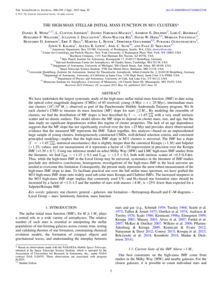
difference in the number of high-mass stars formed, and related
quantities such as commonly used star formation rate (SFR)
indicators. We discuss these implications further in Section 5.3.
For general usage, we recommend the adoption of the
following forms of the the IMF over all stellar masses. With the
M31 high-mass IMF, a modified Chabrier IMF Chabrier
(2003) has the form
m m m
m c m m M
( ) ( ) 0.158 (1 ) exp
( ) , 1.45 , for 1.0 100 ,
(3)
( 1)
0.06
0.03
m(log( ) log(0.08))2
2 0.692
and a modified Kroupa (2001) IMF has the form
m cm
m M
m M
m M
( )
0.3 for 0.08 0.5
1.3 for 0.5 1.0
1.45 , for 1.0 100 .
(4)
( 1)
0.06
0.03
Here we have made two extrapolations to match conven-
tional IMF definitions in the literature. First, we have
extrapolated the M31 IMF down to 1 Me. For most practical
purposes, this extension from 2 Me to 1 Me affects the
resulting stellar mass spectrum at the level of a few percent.
Second, we have extrapolated the M31 IMF up to 100 Me.
While our data do not provide good constraints above
∼25 Me (see Section 1.2), there is little other information to
go on for mass spectra of the most massive stars. Thus, as is
commonplace in the literature, we suggest extrapolating the
M31 IMF up to the highest masses, but recognize that
systematic spectroscopic searches for the massive stars are
absolutely critical for understanding the IMF of the most
massive stars (e.g., Massey et al. 1995b; Massey 2003).
Finally, we have assumed that the sub-solar IMF in M31 is
similar to that of the Galaxy. Although not confirmed by direct
star counts, Conroy & van Dokkum (2012) have shown that
spectral features sensitive to the low-mass IMF yield a result
that is similar to the low-mass Galactic IMF.
5.3. Broader Implications
In Figure 7 we illustrate the mass spectra of high-mass stars
predicted by various commonly used IMF models. The plot
shows the number of stars expected relative to a Kroupa IMF
( 1.3) as a function of mass. For fair comparison, the
slopes have all been normalized at 2 Me, the lower main
sequence mass limit of the PHAT data, and extended to
100 Me on the upper end. We chose this normalization, as
opposed to 1 Me to discuss our ability to distinguish different
forms of the IMF in the literature over the dynamic mass range
of the PHAT data, which is indicate by the vertical dashed
lines. As previously discussed, the indicated upper limit
(25 Me) is likely a lower bound due to the inability of
optical-only photometry to accurately characterize the most
massive stars.
The M31 high-mass IMF predicts the formation of fewer
stars than Kroupa at all masses. The red solid line presents our
median IMF model and shows that the fractional deficit varies
from ∼0.9 at ∼10 Me to ∼0.7 at 100 Me. The red shaded
region reflects the 68% confidence interval in the number of
predicted high-mass stars due to uncertainty on the mean high-
mass IMF slope in M31. At most masses, the uncertainty
deviates from the median by ± ∼5%, but increases to ±15%
for stars >50 Me.
The M31 high-mass IMF is similar to other high-mass IMF
models in the literature. It is particularly close to the Kennicutt
IMF ( 1.5; Kennicutt 1983). It is also the same as the IMF
of Miller & Scalo (1979) over the 1–10 Me range. The
steepness of the Miller & Scalo (1979) IMF above 10 Me is
known to be too extreme (e.g., Kennicutt 1983; Kennicutt et al.
1994). Further, the high-mass IMF from Scalo (1986) has a
similar slope ( 1.6) above ∼4 Me, but a much steeper slope
below it. Finally, the M31 high-mass IMF predicts fewer high-
mass stars than a Salpter IMF for masses >2 Me.
We further quantify differences in these IMF models in
Table 4. Here we have computed the expected number of stars
per 106
Me formed at selected stellar masses assuming a
Kroupa (2001) IMF below 2 Me and the listed IMFs above
2 Me. This table solidifies many of the above points regarding
differences in commonly used high-mass IMF models. It also
highlights an important implication for core collapse super-
novae, whose progenitors are believed to have masses
8 Me(e.g., Smartt 2009). For example, the median M31
high-mass IMF model predicts ∼25% fewer stars with masses
8 Me compared to a Kroupa IMF.
Finally, we consider the implications for commonly used
SFR indicators (e.g., Kennicutt 1998b; Kennicutt & Evans
2012). Using the Flexible Stellar Population Synthesis code
(Conroy et al. 2009, 2010), we compute the luminosity to SFR
conversion coefficients for GALEX far- and near-UV luminos-
ities, along with Hα, which we list in Table 5. To do this, we
have assumed a constant SFH over the last 1 Gyr, the indicated
IMF, mass limits from 0.08 to 100 Me, and case B
recombination to convert the number of ionizing photons to
Hα luminosity. From Kennicutt & Evans (2012) the canonical
conversion from luminosity to SFR can be written as
( )M M L Clog ˙ yr log log (5)x x
1
Figure 7. Number of stars predicted by various common IMF models, relative
to Kroupa (dashed line). The vertical dotted lines indicate the mass range over
which the high-mass IMF was measured in M31. Our median IMF (solid red
line) is essentially identical to that of Kennicutt (1983) ( 1.5Kennicutt ).
However, we also find a small spread, which is indicated by the red band. Our
IMF model indicates a modest deficit of stars >2 Me relative to the canonical
Kroupa IMF.
10

Table4
NumberandFractionofMassiveStarsforDifferentIMFs
IMF⩾NM2⩾NM8⩾NM20⩾NM50⩾NM90Frac.⩾2MFrac.⩾8MFrac.⩾20MFrac.⩾50MFrac.⩾90M
M
10stars
10
4
6
M
10stars
10
4
6
M
10stars
10
3
6
M
10stars
10
2
6
M
10stars
10
1
6
(1)(2)(3)(4)(5)(6)(7)(8)(9)(10)(11)
Kroupa6.91.13.06.26.311111
Salpeter6.81.02.75.45.30.970.900.870.840.83
Weiszetal.6.70.0
0.1
0.880.04
0.08
2.20.2
0.3
4.00.4
0.8
3.80.4
0.9
0.900.01
0.04
0.740.04
0.09
0.660.06
0.11
0.600.07
0.13
0.560.06
0.14
Kennicutt6.70.821.93.53.20.870.670.570.500.46
Miller&Scalo6.80.660.820.810.560.850.510.230.110.08
Scalo5.60.200.430.720.650.540.140.100.080.07
Note.Thenumberofexpectedstarsabovethespeciﬁedmasslimitper106
Me.Forthesecalculations,wehaveadoptedaKroupa(2001)IMFbelow2Me,thespeciﬁedIMFabove2Me,andassumedlowerandupper
massboundsforthetotalIMFtobe0.08Meand100Me.Columns(7)–(11)givethefractionofstarsformedabovethelistedmass,relativetothestandardKroupaIMF.
11

where M˙ is the SFR, Lx is the luminosity over the bandpass x,
and Cx is the conversion constant over the same wavelength
range. We have provided updated values for Cx in Table 5.
From column (5) of Table 5, we see modest differences in
the SFR indicators due to an M31 high-mass IMF. The
variations are such that for a fixed luminosity, using the M31
high-mass IMF results in SFRs that are a factor ∼1.3–1.5
larger.
Although the change in absolute calibration is modest, the
IMF measurement in M31 provides a significant increase in the
precision of the SFR. Including uncertainties the high-mass
Kroupa IMF slope is 1.3 0.7. Propagating this
uncertainty through Equation (5) results in an order of
magnitude uncertainty in Hα SFRs. In contrast, the precision
of our IMF measurement in M31 reduces this uncertainty to be
of the order unity, representing a substantial improvement in
our knowledge of galaxy SFRs (under the assumption of a
universal IMF).
The authors would like to thank the anonymous referee for a
careful reading of the paper and insightful comments. D.R.W.
also thanks Nate Bastian, Charlie Conroy, Rob Kennicutt, and
John Saclo for their useful comments on this paper and
discussions about the IMF and its history. Support for this work
was provided by NASA through grant number HST GO-12055
from the Space Telescope Science Institute, which is operated
by AURA, Inc., under NASA contract NAS5-26555. D.R.W. is
supported by NASA through Hubble Fellowship grant HST-
HF-51331.01 awarded by the Space Telescope Science
Institute. D.R.W. also wishes to thank the MPIA and KITP
for their generous hospitality during the writing of this paper.
This work used the Extreme Science and Engineering
Discovery Environment (XSEDE), which is supported by
National Science Foundation grant number ACI-1053575, was
supported in part by the National Science Foundation under
Grant No. NSF PHY11-25915, and made extensive use of
NASA’s Astrophysics Data System Bibliographic Services. In
large part, analysis and plots presented in this paper utilized
IPython and packages from NumPy, SciPy, and Matplotlib
(Hunter 2007; Oliphant 2007; Pérez & Granger 2007; Astropy
Collaboration et al. 2013).
APPENDIX
In this Appendix, we have tabulated the MF slopes for each
cluster used in this study. The APID numbers listed in Table 6
can be used to cross-correlate the MF slopes with other cluster
properties as listed in L. Beerman et al. (2015, in preparation).
We plan to publish a larger study of cluster MFs in M31,
including 1000 star clusters. In this paper, we will include a full
table of MFs and cluster age/mass/extinction/size, etc.
REFERENCES
Alves, J., Lombardi, M., & Lada, C. J. 2007, A&A, 462, L17
Andrews, J. E., Calzetti, D., Chandar, R., et al. 2013, ApJ, 767, 51
Ascenso, J., Alves, J., & Lago, M. T. V. T. 2009, Ap&SS, 324, 113
Astropy Collaboration, Robitaille, T. P., Tollerud, E. J., et al. 2013, A&A,
558, A33
Audouze, J., & Tinsley, B. M. 1976, ARA&A, 14, 43
Baldry, I. K., & Glazebrook, K. 2003, ApJ, 593, 258
Banerjee, S., & Kroupa, P. 2012, A&A, 547, A23
Bastian, N., Covey, K. R., & Meyer, M. R. 2010, ARA&A, 48, 339
Belczynski, K., Buonanno, A., Cantiello, M., et al. 2014, ApJ, 789, 120
Boselli, A., Boissier, S., Cortese, L., et al. 2009, ApJ, 706, 1527
Calzetti, D., Chandar, R., Lee, J. C., et al. 2010, ApJL, 719, L158
Chabrier, G. 2003, PASP, 115, 763
Conroy, C. 2013, ARA&A, 51, 393
Conroy, C., Gunn, J. E., & White, M. 2009, ApJ, 699, 486
Conroy, C., & van Dokkum, P. G. 2012, ApJ, 760, 71
Conroy, C., White, M., & Gunn, J. E. 2010, ApJ, 708, 58
da Silva, R. L., Fumagalli, M., & Krumholz, M. 2012, ApJ, 745, 145
Dalcanton, J. J., Williams, B. F., Lang, D., et al. 2012, ApJS, 200, 18
Davé, R. 2011, in ASP Conf. Ser. 440, UP2010: Have Observations Revealed a
Variable Upper End of the Initial Mass Function? ed. M. Treyer et al. (San
Francisco, CA: ASP), 353
de La Fuente Marcos, R. 1997, A&A, 322, 764
De Marchi, G., Paresce, F., & Portegies Zwart, S. 2010, ApJ, 718, 105
de Mink, S. E., Sana, H., Langer, N., Izzard, R. G., & Schneider, F. R. N. 2014,
ApJ, 782, 7
Dib, S. 2014, MNRAS, 444, 1957
Dolphin, A. E. 2000, PASP, 112, 1383
Dolphin, A. E. 2002, MNRAS, 332, 91
Draine, B. T., Aniano, G., Krause, O., et al. 2013, arXiv:1306.2304
Eisenhauer, F. 2001, in Starburst Galaxies Near and Far, ed. L. Tacconi &
D. Lutz (Berlin: Springer-Verlag), 24
Elmegreen, B. G. 1999, ApJ, 515, 323
Elmegreen, B. G. 2006, arXiv:astro-ph/0610687
Elmegreen, B. G., & Scalo, J. 2006, ApJ, 636, 149
Elson, R. A. W., Sigurdsson, S., Davies, M., Hurley, J., & Gilmore, G. 1998,
MNRAS, 300, 857
Fardal, M. A., Katz, N., Weinberg, D. H., & Davé, R. 2007, MNRAS, 379, 985
Foreman-Mackey, D., Hogg, D. W., Lang, D., & Goodman, J. 2013, PASP,
125, 306
Table 5
Updated Broadband SFR Indicators
Band Lx Units Log(Cx) Log(Cx) M M M˙ ( 31) ˙ (Kroupa)
(Kroupa) (M31)
(1) (2) (3) (4) (5)
FUV erg s−1
( L ) 43.29 43.18 0.02
0.05
1.28 0.12
0.06
NUV erg s−1
( L ) 43.14 43.04 0.02
0.03
1.24 0.11
0.06
Hα erg s−1
40.91 40.73 0.07
0.04
1.52 0.24
0.13
Note. A comparison of commonly used SFR indicators for a Kroupa and M31
IMF values. The values of Lx, Cx, and M˙ follow Kennicutt & Evans (2012)
and Equation (5).
Table 6
MF Slopes for Each Cluster
APID Median Γ Upper 68% Uncertainty Lower 68% Uncertainty
(1) (2) (3) (4)
94 1.37 0.31 0.32
98 2.21 0.37 0.9
111 0.01 1.48 1.55
249 1.36 0.67 0.8
266 1.4 0.27 0.28
285 1.26 0.25 0.24
323 1.05 0.39 0.42
390 1.89 0.26 0.32
403 1.39 0.19 0.23
431 1.45 0.38 0.41
447 1.27 0.72 1.24
452 2.39 0.41 0.41
462 0.09 0.84 0.82
522 1.36 0.29 0.29
552 1.46 0.17 0.17
Note. The cluster MFs used in this study. Values in column (2) represent the
median of the marginalized PDF for each cluster’s MF slope. Columns (3) and
(4) indicate the upper and lower 68% confidence intervals.
12

Foreman-Mackey, D., Hogg, D. W., & Morton, T. D. 2014, arXiv:1406.3020
Fumagalli, M., da Silva, R. L., & Krumholz, M. R. 2011, ApJL, 741, L26
Gallart, C., Zoccali, M., & Aparicio, A. 2005, ARA&A, 43, 387
Gilmore, G. 2001, in Starburst Galaxies Near and Far ed. L. Tacconi & D. Lutz
(Berlin: Springer-Verlag), 34
Girardi, L., Bertelli, G., Bressan, A., et al. 2002, A&A, 391, 195
Girardi, L., Williams, B. F., Gilbert, K. M., et al. 2010, ApJ, 724, 1030
Hogg, D. W., Myers, A. D., & Bovy, J. 2010, ApJ, 725, 2166
Hopkins, P. F. 2013, MNRAS, 433, 170
Hoversten, E. A., & Glazebrook, K. 2008, ApJ, 675, 163
Hunter, J. D. 2007, CSE, 9, 90
Jaschek, C., & Jaschek, M. 1957, PASP, 69, 337
Johnson, L. C., Seth, A. C., Dalcanton, J. J., et al. 2012, ApJ, 752, 95
Johnson, L. C., Seth, A. C., Dalcanton, J. J., et al. 2015, arXiv:1501.04966
Kennicutt, R. C., & Evans, N. J. 2012, ARA&A, 50, 531
Kennicutt, R. C., Jr. 1983, ApJ, 272, 54
Kennicutt, R. C., Jr. 1998a, in ASP Conf. Ser. 142, The Stellar Initial Mass
Function (38th Herstmonceux Conf.), ed. G. Gilmore & D. Howell (San
Francisco, CA: ASP), 1
Kennicutt, R. C., Jr. 1998b, ARA&A, 36, 189
Kennicutt, R. C., Jr., Tamblyn, P., & Congdon, C. E. 1994, ApJ, 435, 22
Kobulnicky, H. A., Kiminki, D. C., Lundquist, M. J., et al. 2014, ApJS, 213, 34
Kroupa, P. 2001, MNRAS, 322, 231
Kroupa, P. 2002, Sci, 295, 82
Kroupa, P., Weidner, C., Pflamm-Altenburg, J., et al. 2013, in The Stellar and
Sub-Stellar Initial Mass Function of Simple and Composite Populations, ed.
T. D. Oswalt & G. Gilmore (Dordrecht: Springer Netherlands), 115
Kruijssen, J. M. D. 2009, A&A, 507, 1409
Krumholz, M. R. 2014, arXiv:1402.0867
Lee, J. C., Gil de Paz, A., Tremonti, C., et al. 2009, ApJ, 706, 599
Leitherer, C. 1998, in ASP Conf. Seri. 142, The Stellar Initial Mass Function,
(38th Herstmonceux Conf.), ed. G. Gilmore & D. Howell, 61
Lequeux, J. 1979, A&A, 80, 35
Lewis, A. R., Dolphin, A. E., Dalcanton, J. J., et al. 2015, arXiv:1504.03338
Limber, D. N. 1960, ApJ, 131, 168
Madau, P., & Dickinson, M. 2014, ARA&A, 52, 415
Maíz Apellániz, J. 2008, ApJ, 677, 1278
Maíz Apellániz, J., & Úbeda, L. 2005, ApJ, 629, 873
Marigo, P., Girardi, L., Bressan, A., et al. 2008, A&A, 482, 883
Massey, P. 1998, in ASP Conf. Ser. 142, The Stellar Initial Mass Function
(38th Herstmonceux Conf.), ed. G. Gilmore & D. Howell (San Francisco,
CA: ASP), 17
Massey, P. 2003, ARA&A, 41, 15
Massey, P. 2011, in ASP Conf. Ser. 440, UP2010: Have Observations
Revealed a Variable Upper End of the Initial Mass Function?, ed. M. Treyer
et al. (San Francisco, CA: ASP), 29
Massey, P., Johnson, K. E., & Degioia-Eastwood, K. 1995a, ApJ, 454, 151
Massey, P., Lang, C. C., Degioia-Eastwood, K., & Garmany, C. D. 1995b,
ApJ, 438, 188
Mateo, M. 1993, in ASP Conf. Ser. 48, The Globular Cluster-Galaxy
Connection, ed. G. H. Smith & J. P. Brodie (San Francisco, CA: ASP), 387
McConnachie, A. W., Irwin, M. J., Ferguson, A. M. N., et al. 2005, MNRAS,
356, 979
McKee, C. F., & Ostriker, E. C. 2007, ARA&A, 45, 565
Meurer, G. R., Wong, O. I., Kim, J. H., et al. 2009, ApJ, 695, 765
Miller, G. E., & Scalo, J. M. 1979, ApJS, 41, 513
Narayanan, D., & Davé, R. 2012, MNRAS, 423, 3601
Narayanan, D., & Davé, R. 2013, MNRAS, 436, 2892
Oh, S., Kroupa, P., & Pflamm-Altenburg, J. 2015a, arXiv:1503.08827
Oh, S.-H., Hunter, D. A., Brinks, E., et al. 2015b, arXiv:1502.01281v1
Oliphant, T. E. 2007, CSE, 9, 10
Ostriker, J. P., Richstone, D. O., & Thuan, T. X. 1974, ApJL, 188, L87
Pérez, F., & Granger, B. E. 2007, CSE, 9, 21
Pflamm-Altenburg, J., & Kroupa, P. 2009, ApJ, 706, 516
Phelps, R. L., & Janes, K. A. 1993, AJ, 106, 1870
Portegies Zwart, S. F., McMillan, S. L. W., & Gieles, M. 2010, ARA&A,
48, 431
Salpeter, E. E. 1955, ApJ, 121, 161
Salpeter, E. E. 2005, in The Initial Mass Function 50 Years Later, Vol. 327, ed.
E. Corbelli, F. Palla & H. Zinnecker (Dordrecht: Springer Netherlands), 3
Sana, H., de Koter, A., de Mink, S. E., et al. 2013, A&A, 550, A107
Sandage, A. 1957, ApJ, 125, 422
Sanders, N. E., Caldwell, N., McDowell, J., & Harding, P. 2012, ApJ, 758, 133
Scalo, J. 1998, in ASP Conf. Ser. 142, The Stellar Initial Mass Function (38th
Herstmonceux Conf.) ed. G. Gilmore & D. Howell (San Francisco, CA:
ASP), 201
Scalo, J. 2005, in The Initial Mass Function 50 Years Later, Vol. 327, ed.
E. Corbelli, F. Palla & H. Zinnecker (Dordrecht: Springer
Netherlands), 23
Scalo, J. M. 1986, FCPh, 11, 1
Schmidt, M. 1959, ApJ, 129, 243
Schneider, F. R. N., Izzard, R. G., Langer, N., & de Mink, S. E. 2015,
arXiv:1504.01735
Searle, L., Sargent, W. L. W., & Bagnuolo, W. G. 1973, ApJ, 179, 427
Smartt, S. J. 2009, ARA&A, 47, 63
Stetson, P. B. 1987, PASP, 99, 191
Taff, L. G. 1974, AJ, 79, 1280
Talbot, R. J., Jr., & Arnett, W. D. 1973, ApJ, 186, 51
Tarrab, I. 1982, A&A, 109, 285
Tinsley, B. M. 1968, ApJ, 151, 547
Trundle, C., Dufton, P. L., Lennon, D. J., Smartt, S. J., & Urbaneja, M. A.
2002, A&A, 395, 519
van den Bergh, S. 1957, ApJ, 125, 445
van den Bergh, S., & Sher, D. 1960, PDDO, 2, 203
Venn, K. A., McCarthy, J. K., Lennon, D. J., et al. 2000, ApJ, 541, 610
Weidner, C., & Kroupa, P. 2005, ApJ, 625, 754
Weidner, C., Kroupa, P., & Maschberger, T. 2009, MNRAS, 393, 663
Weidner, C., Kroupa, P., & Pflamm-Altenburg, J. 2014, MNRAS, 441, 3348
Weisz, D. R., Johnson, B. D., Johnson, L. C., et al. 2012, ApJ, 744, 44
Weisz, D. R., Fouesneau, M., Hogg, D. W., et al. 2013, ApJ, 762, 123
Wilkins, S. M., Trentham, N., & Hopkins, A. M. 2008, MNRAS, 385, 687
Williams, B. F., Lang, D., Dalcanton, J. J., et al. 2014, ApJS, 215, 9
Zinnecker, H. 2005, in The Initial Mass Function 50 Years Later, Vol. 327,
ed. E. Corbelli, F. Palla & H. Zinnecker (Dordrecht: Springer
Netherlands), 19
Zurita, A., & Bresolin, F. 2012, MNRAS, 427, 1463
13

The high mass_stelar_initial_mass_function_in_m31_clusters

Recommended

Recommended

More Related Content

What's hot

What's hot (20)

Viewers also liked

Viewers also liked (17)

Similar to The high mass_stelar_initial_mass_function_in_m31_clusters

Similar to The high mass_stelar_initial_mass_function_in_m31_clusters (20)

More from Sérgio Sacani

More from Sérgio Sacani (20)

Recently uploaded

Recently uploaded (20)

The high mass_stelar_initial_mass_function_in_m31_clusters