SlideShare a Scribd company logo
1 of 18
Download to read offline
Solved with COMSOL Multiphysics 5.1
1 | S T R E S S E S A N D H E A T G E N E R A T I O N I N L A N D I N G G E A R
Stresses and Heat Generation in
Landing Gear
Introduction
This model simulates the dynamics of the shock absorber used in a landing gear
mechanism using the Multibody Dynamics interface present in COMSOL
Multiphysics. It analyzes the stresses in the landing gear components and the energy
dissipated in the absorber during the landing of an aircraft. The heat transfer analysis
is also performed, in which the rise of temperature in the components due to heat
generated in the shock absorber is calculated by coupling the Multibody Dynamics
interface with the Heat Transfer in Solids interface.
Model Definition
The landing gear assembly, shown in Figure 1, consists of two tires, a shock-absorber
piston, and a shock-absorber cylinder. Other components in the landing gear, which
are not relevant in this analysis, are not modeled.
Shock-absorber cylinder
Shock-absorber piston
Tire
Figure 1: Geometry of the landing gear.
Solved with COMSOL Multiphysics 5.1
2 | S T R E S S E S A N D H E A T G E N E R A T I O N I N L A N D I N G G E A R
The shock-absorber piston and cylinder are connected through a prismatic joint that
has only one translational degree of freedom. The joint is loaded with a spring and a
damper to absorb the shock during the landing. This is modeled using the spring and
damper subnode of the prismatic joint.
To model the effect of the tires, the bottom surfaces of the shock-absorber piston are
loaded with equivalent spring and damper. The energy dissipated in the damper is used
as a heat source on the common boundaries of the shock-absorber piston and cylinder.
Remaining boundaries are considered to be insulated. The heat generated on the
boundaries is conducted into the landing gear components during the landing, which
increases their temperature.
Results and Discussion
Figure 2 displays the stress generated in the landing gear components at the time when
the displacement reaches its maximum.
Figure 2: von Mises stress distribution in the deformed landing gear.
Figure 3 shows the relative displacement between the shock-absorber piston and
cylinder during landing. The amplitude of the relative displacement is very high
initially, but it decays rapidly due to the energy loss in the shock absorber and tires.
Solved with COMSOL Multiphysics 5.1
3 | S T R E S S E S A N D H E A T G E N E R A T I O N I N L A N D I N G G E A R
Figure 3: Relative displacement between the shock-absorber piston and cylinder.
Figure 4: Relative velocity between the shock-absorber piston and cylinder.
Solved with COMSOL Multiphysics 5.1
4 | S T R E S S E S A N D H E A T G E N E R A T I O N I N L A N D I N G G E A R
Figure 4 shows the relative velocity variation between the shock-absorber piston and
cylinder during landing. The relative velocity is also very high initially, and it decays to
zero due to the energy loss in shock absorber and tires during the course of landing.
The force component in y direction in the prismatic joint is shown in Figure 5. The
force also decays with time and subsequently acquires a steady state value equivalent to
the weight of the whole supported system.
Figure 6 shows the variation in the energy components during the landing. Initially,
the kinetic energy is very high. But due to the dissipation in the subsequent cycles, it
decays to zero. The other forms of energies, such as strain energy and potential energy,
are very small as compared to the kinetic energy. This happens because most of the
kinetic energy is stored in the shock absorber initially and then dissipated before
getting converted to any other forms of energy.
The temperature rise in the components due to heat dissipated in shock-absorber is
shown in Figure 7. The maximum temperature rise occurs near the piston-cylinder
boundaries.
Figure 5: The y component of force in the shock-absorber.
Solved with COMSOL Multiphysics 5.1
5 | S T R E S S E S A N D H E A T G E N E R A T I O N I N L A N D I N G G E A R
Figure 6: Variation of different types of energy in the gear during landing.
Figure 7: Temperature profile in the landing gear.
Solved with COMSOL Multiphysics 5.1
6 | S T R E S S E S A N D H E A T G E N E R A T I O N I N L A N D I N G G E A R
Application Library path: Multibody_Dynamics_Module/
Automotive_and_Aerospace/landing_gear
Modeling Instructions
From the File menu, choose New.
N E W
1 In the New window, click Model Wizard.
M O D E L W I Z A R D
1 In the Model Wizard window, click 2D.
2 In the Select physics tree, select Structural Mechanics>Multibody Dynamics (mbd).
3 Click Add.
4 In the Select physics tree, select Heat Transfer>Heat Transfer in Solids (ht).
5 Click Add.
6 Click Study.
7 In the Select study tree, select Preset Studies for Selected Physics Interfaces>Time
Dependent.
8 Click Done.
G L O B A L D E F I N I T I O N S
Parameters
1 On the Home toolbar, click Parameters.
2 In the Settings window for Parameters, locate the Parameters section.
3 In the table, enter the following settings:
Name Expression Value Description
m 5000[kg] 5000 kg Mass of the aircraft
vi 10[m/s] 10 m/s Downward velocity of
the aircraft
k_sa 2.5e6[N/m] 2.5E6 N/m Spring constant of
shock absorber
Solved with COMSOL Multiphysics 5.1
7 | S T R E S S E S A N D H E A T G E N E R A T I O N I N L A N D I N G G E A R
If you do not want to build all the geometry, you can load the geometry sequence from
the stored model. In the Model Builder window, under Component 1 right-click
Geometry 1 and choose Insert Sequence from File. Browse to the applicationโ€™s
Application Library folder and double-click the file landing_gear.mph. You can then
continue to the Add Material section below.
To build the geometry from a scratch, continue here.
G E O M E T R Y 1
Circle 1 (c1)
1 On the Geometry toolbar, click Primitives and choose Circle.
2 In the Settings window for Circle, locate the Size and Shape section.
3 In the Radius text field, type 0.15.
4 Locate the Position section. In the x text field, type -0.3.
Bรฉzier Polygon 1 (b1)
1 On the Geometry toolbar, click Primitives and choose Bรฉzier Polygon.
2 In the Settings window for Bรฉzier Polygon, locate the Polygon Segments section.
3 Find the Added segments subsection. Click Add Linear.
4 Find the Control points subsection. In row 1, set x to -0.35.
5 In row 2, set x to -0.35.
6 In row 2, set y to 0.3.
7 Find the Added segments subsection. Click Add Linear.
8 Find the Control points subsection. In row 2, set x to -0.15.
9 In row 2, set y to 0.4.
10 Find the Added segments subsection. Click Add Linear.
11 Find the Control points subsection. In row 2, set x to -0.05.
12 Find the Added segments subsection. Click Add Linear.
c_sa 5e4[N*s/m] 5E4 Nยทs/m Damping coefficient of
shock absorber
k_t 2.5e7[N/m] 2.5E7 N/m Stiffness of tyre
c_t 2.5e6[N*s/m] 2.5E6 Nยทs/m Damping coefficient of
tyre
d 0.1[m] 0.1 m Out of plane dimension
Name Expression Value Description
Solved with COMSOL Multiphysics 5.1
8 | S T R E S S E S A N D H E A T G E N E R A T I O N I N L A N D I N G G E A R
13 Find the Control points subsection. In row 2, set y to 1.
14 Find the Added segments subsection. Click Add Linear.
15 Find the Control points subsection. In row 2, set x to 0.
16 Find the Added segments subsection. Click Add Linear.
17 Find the Control points subsection. In row 2, set y to 0.3.
18 Find the Added segments subsection. Click Add Linear.
19 Find the Control points subsection. In row 2, set x to -0.15+0.1*(sqrt(5)-2).
20 Find the Added segments subsection. Click Add Linear.
21 Find the Control points subsection. In row 2, set x to -0.25.
22 In row 2, set y to 0.3-0.05*(sqrt(5)-1).
23 Find the Added segments subsection. Click Add Linear.
24 Find the Control points subsection. In row 2, set y to 0.
Bรฉzier Polygon 2 (b2)
1 On the Geometry toolbar, click Primitives and choose Bรฉzier Polygon.
2 In the Settings window for Bรฉzier Polygon, locate the Polygon Segments section.
3 Find the Added segments subsection. Click Add Linear.
4 Find the Control points subsection. In row 1, set x to -0.15.
5 In row 1, set y to 0.8.
6 In row 2, set x to -0.15.
7 In row 2, set y to 1.3+0.1*sqrt(2).
8 Find the Added segments subsection. Click Add Linear.
9 Find the Control points subsection. In row 2, set x to -0.05.
10 In row 2, set y to 1.4+0.1*sqrt(2).
11 Find the Added segments subsection. Click Add Linear.
12 Find the Control points subsection. In row 2, set y to 1.8.
13 Find the Added segments subsection. Click Add Linear.
14 Find the Control points subsection. In row 2, set x to 0.
15 Find the Added segments subsection. Click Add Linear.
16 Find the Control points subsection. In row 2, set y to 1.4.
17 Find the Added segments subsection. Click Add Linear.
18 Find the Control points subsection. In row 2, set x to -0.05.
Solved with COMSOL Multiphysics 5.1
9 | S T R E S S E S A N D H E A T G E N E R A T I O N I N L A N D I N G G E A R
19 Find the Added segments subsection. Click Add Linear.
20 Find the Control points subsection. In row 2, set y to 0.8.
21 Right-click Component 1 (comp1)>Geometry 1>Bรฉzier Polygon 2 (b2) and choose
Build Selected.
22 Click the button on the Graphics toolbar.
23 Click the Zoom Extents button on the Graphics toolbar.
Copy 1 (copy1)
1 On the Geometry toolbar, click Transforms and choose Copy.
2 Select the object b1 only.
Difference 1 (dif1)
1 On the Geometry toolbar, click Booleans and Partitions and choose Difference.
2 Select the object c1 only.
3 In the Settings window for Difference, locate the Difference section.
4 Find the Objects to subtract subsection. Select the Active toggle button.
5 Select the object copy1 only.
Mirror 1 (mir1)
1 On the Geometry toolbar, click Transforms and choose Mirror.
2 Click in the Graphics window and then press Ctrl+A to select all objects.
3 In the Settings window for Mirror, locate the Input section.
4 Select the Keep input objects check box.
Union 1 (uni1)
1 On the Geometry toolbar, click Booleans and Partitions and choose Union.
2 Select the objects b1 and mir1(1) only.
3 In the Settings window for Union, locate the Union section.
4 Clear the Keep interior boundaries check box.
Union 2 (uni2)
1 On the Geometry toolbar, click Booleans and Partitions and choose Union.
2 Select the objects mir1(2) and b2 only.
3 In the Settings window for Union, locate the Union section.
4 Clear the Keep interior boundaries check box.
Solved with COMSOL Multiphysics 5.1
10 | S T R E S S E S A N D H E A T G E N E R A T I O N I N L A N D I N G G E A R
Union 3 (uni3)
1 On the Geometry toolbar, click Booleans and Partitions and choose Union.
2 Select the objects uni1, mir1(3), and dif1 only.
Form Union (fin)
1 In the Model Builder window, under Component 1 (comp1)>Geometry 1 click Form
Union (fin).
2 In the Settings window for Form Union/Assembly, locate the Form Union/Assembly
section.
3 From the Action list, choose Form an assembly.
4 Right-click Component 1 (comp1)>Geometry 1>Form Union (fin) and choose Build
Selected.
5 Click the Go to Default 3D View button on the Graphics toolbar.
6 Click the Zoom Extents button on the Graphics toolbar.
A D D M A T E R I A L
1 On the Home toolbar, click Add Material to open the Add Material window.
2 Go to the Add Material window.
3 In the tree, select Built-In>Structural steel.
4 Click Add to Component in the window toolbar.
5 On the Home toolbar, click Add Material to close the Add Material window.
M U L T I B O D Y D Y N A M I C S ( M B D )
1 In the Model Builder window, under Component 1 (comp1) click Multibody Dynamics
(mbd).
2 In the Settings window for Multibody Dynamics, locate the Thickness section.
3 In the d text field, type d.
Initial Values 1
1 In the Model Builder window, under Component 1 (comp1)>Multibody Dynamics
(mbd) click Initial Values 1.
2 In the Settings window for Initial Values, locate the Initial Values section.
3 From the list, choose Locally defined.
Solved with COMSOL Multiphysics 5.1
11 | S T R E S S E S A N D H E A T G E N E R A T I O N I N L A N D I N G G E A R
4 Specify the โˆ‚u/โˆ‚t vector as
Attachment 1
1 On the Physics toolbar, click Boundaries and choose Attachment.
2 Select Boundaries 34 and 40 only.
Attachment 2
1 On the Physics toolbar, click Boundaries and choose Attachment.
2 Select Boundaries 10 and 14 only.
Prismatic Joint 1
1 On the Physics toolbar, click Global and choose Prismatic Joint.
2 In the Settings window for Prismatic Joint, locate the Attachment Selection section.
3 From the Source list, choose Attachment 1.
4 From the Destination list, choose Attachment 2.
5 Locate the Axis of Joint section. Specify the e0 vector as
Spring and Damper 1
1 On the Physics toolbar, click Attributes and choose Spring and Damper.
2 In the Settings window for Spring and Damper, locate the Spring and Damper:
Translational section.
3 In the ku text field, type k_sa.
4 In the cu text field, type c_sa.
Use the Added Mass node to account for the mass of the aircraft.
Added Mass 1
1 On the Physics toolbar, click Boundaries and choose Added Mass.
2 Select Boundaries 37 and 39 only.
3 In the Settings window for Added Mass, locate the Added Mass section.
4 From the Mass type list, choose Total mass.
0 X
-vi Y
0 x
-1 y
Solved with COMSOL Multiphysics 5.1
12 | S T R E S S E S A N D H E A T G E N E R A T I O N I N L A N D I N G G E A R
5 Specify the m vector as
Gravity 1
1 On the Physics toolbar, click Domains and choose Gravity.
2 In the Settings window for Gravity, locate the Domain Selection section.
3 From the Selection list, choose All domains.
The Spring Foundation node is used to account for the elastic and damping effects of
the tyres.
Spring Foundation 1
1 On the Physics toolbar, click Boundaries and choose Spring Foundation.
2 Select Boundaries 2 and 19 only.
3 In the Settings window for Spring Foundation, locate the Spring section.
4 From the Spring type list, choose Total spring constant.
5 From the list, choose Diagonal.
6 In the ktot table, enter the following settings:
7 Click to expand the Viscous damping section. Locate the Viscous Damping section.
From the Damping type list, choose Total damping constant.
8 From the list, choose Diagonal.
9 In the dtot table, enter the following settings:
D E F I N I T I O N S
Integration 1 (intop1)
1 On the Definitions toolbar, click Component Couplings and choose Integration.
2 In the Settings window for Integration, locate the Source Selection section.
3 From the Geometric entity level list, choose Boundary.
0 X
m Y
0 0
0 k_t
0 0
0 c_t
Solved with COMSOL Multiphysics 5.1
13 | S T R E S S E S A N D H E A T G E N E R A T I O N I N L A N D I N G G E A R
4 Select Boundaries 10 and 14 only.
Integration 2 (intop2)
1 On the Definitions toolbar, click Component Couplings and choose Integration.
2 In the Settings window for Integration, locate the Source Selection section.
3 From the Selection list, choose All domains.
Variables 1
1 On the Definitions toolbar, click Local Variables.
The heat generated due to the energy dissipation in the absorber is modeled as a
heat source. This heat source is distributed on the common boundaries of the
shock-absorber piston and cylinder.
2 In the Settings window for Variables, locate the Variables section.
3 In the table, enter the following settings:
H E A T TR A N S F E R I N S O L I D S ( H T )
Pair Boundary Heat Source 1
1 On the Physics toolbar, in the Boundary section, click Pairs and choose Pair Boundary
Heat Source.
2 In the Settings window for Pair Boundary Heat Source, locate the Pair Selection
section.
3 In the Pairs list, select Identity Pair 1 (ap1).
4 Locate the Boundary Heat Source section. Click the Overall heat transfer rate button.
5 In the Pb text field, type Q*1[m]/d.
Here, the total power is scaled with the actual out-of-plane thickness to get the
correct temperature distribution.
Name Expression Unit Description
Q mbd.prj1.Qdamper W Heat generated
per second
Wp intop2(mbd.rho*g_const*v*mbd.d) J Potential energy
h_sa timeint(0,t,Q) J Energy loss in
shock-absorber
Ws_sa mbd.prj1.Wspring J Energy stored in
shock-absorber
Solved with COMSOL Multiphysics 5.1
14 | S T R E S S E S A N D H E A T G E N E R A T I O N I N L A N D I N G G E A R
M E S H 1
1 In the Model Builder window, under Component 1 (comp1) click Mesh 1.
2 In the Settings window for Mesh, locate the Mesh Settings section.
3 From the Element size list, choose Finer.
4 Click the Build All button.
S T U D Y 1
Step 1: Time Dependent
1 In the Model Builder window, under Study 1 click Step 1: Time Dependent.
2 In the Settings window for Time Dependent, locate the Study Settings section.
3 In the Times text field, type range(0,0.01,0.7).
4 On the Home toolbar, click Compute.
R E S U L T S
Displacement (mbd)
Follow these instructions to generate a plot similar to that is shown in Figure 2:
1 In the Model Builder window, click Displacement (mbd).
2 In the Settings window for 2D Plot Group, type Stress in the Label text field.
3 Locate the Plot Settings section. From the Frame list, choose Material (X, Y, Z).
4 Locate the Data section. From the Time (s) list, choose 0.06.
Stress
1 In the Model Builder window, expand the Results>Stress node, then click Surface 1.
2 In the Settings window for Surface, click Replace Expression in the upper-right corner
of the Expression section. From the menu, choose Component 1>Multibody
Dynamics>Stress>mbd.mises - von Mises stress.
3 Click to expand the Quality section. From the Resolution list, choose No refinement.
4 On the Stress toolbar, click Plot.
5 Click the Zoom Extents button on the Graphics toolbar.
Follow these instructions to generate a plot similar to that is shown in Figure 7:
Temperature (ht)
1 In the Model Builder window, expand the Results>Temperature (ht) node, then click
Surface 1.
Solved with COMSOL Multiphysics 5.1
15 | S T R E S S E S A N D H E A T G E N E R A T I O N I N L A N D I N G G E A R
2 In the Settings window for Surface, locate the Quality section.
3 From the Resolution list, choose No refinement.
4 Right-click Results>Temperature (ht)>Surface 1 and choose Deformation.
5 In the Settings window for Deformation, locate the Scale section.
6 Select the Scale factor check box.
7 In the associated text field, type 1.
8 On the Temperature (ht) toolbar, click Plot.
Follow these instructions to generate a relative displacement plot similar to that is
shown in Figure 3:
1D Plot Group 5
1 On the Home toolbar, click Add Plot Group and choose 1D Plot Group.
2 In the Settings window for 1D Plot Group, type Relative displacement in the
Label text field.
3 Click to expand the Title section. From the Title type list, choose None.
Relative displacement
1 On the Relative displacement toolbar, click Global.
2 In the Settings window for Global, click Replace Expression in the upper-right corner
of the y-axis data section. From the menu, choose Component 1>Multibody
Dynamics>Prismatic joints>Prismatic Joint 1>mbd.prj1.u - Relative displacement.
3 Click to expand the Legends section. Clear the Show legends check box.
4 Click to expand the Coloring and style section. Locate the Coloring and Style section.
Find the Line style subsection. In the Width text field, type 2.
5 On the Relative displacement toolbar, click Plot.
Follow these instructions to generate a relative velocity plot similar to that is shown in
Figure 4:
Relative displacement 1
1 In the Model Builder window, right-click Relative displacement and choose Duplicate.
2 In the Settings window for 1D Plot Group, type Relative velocity in the Label
text field.
Relative velocity
1 In the Model Builder window, expand the Results>Relative velocity node, then click
Global 1.
Solved with COMSOL Multiphysics 5.1
16 | S T R E S S E S A N D H E A T G E N E R A T I O N I N L A N D I N G G E A R
2 In the Settings window for Global, click Replace Expression in the upper-right corner
of the y-axis data section. From the menu, choose Component 1>Multibody
Dynamics>Prismatic joints>Prismatic Joint 1>mbd.prj1.u_t - Relative velocity.
3 On the Relative velocity toolbar, click Plot.
Follow these instructions to generate a joint force plot similar to that is shown in
Figure 5:
Relative velocity 1
1 In the Model Builder window, right-click Relative velocity and choose Duplicate.
2 In the Settings window for 1D Plot Group, type Joint Force in the Label text field.
Joint Force
1 In the Model Builder window, expand the Results>Joint Force node, then click Global
1.
2 In the Settings window for Global, click Replace Expression in the upper-right corner
of the y-axis data section. From the menu, choose Component 1>Multibody
Dynamics>Prismatic joints>Prismatic Joint 1>Joint force>mbd.prj1.Fy - Joint force, y
component.
3 On the Joint Force toolbar, click Plot.
To generate energy plot shown in Figure 6, follow the instructions below.
1D Plot Group 8
1 On the Home toolbar, click Add Plot Group and choose 1D Plot Group.
2 In the Settings window for 1D Plot Group, type Energy in the Label text field.
3 Locate the Title section. From the Title type list, choose None.
Energy
1 On the Energy toolbar, click Global.
2 In the Settings window for Global, click Replace Expression in the upper-right corner
of the y-axis data section. From the menu, choose Component
1>Definitions>Variables>Wp - Potential energy.
3 Click Add Expression in the upper-right corner of the y-axis data section. From the
menu, choose Component 1>Multibody Dynamics>Global>mbd.Wk_tot - Total kinetic
energy.
4 Click Add Expression in the upper-right corner of the y-axis data section. From the
menu, choose Component 1>Multibody Dynamics>Global>mbd.Ws_tot - Total elastic
strain energy.
Solved with COMSOL Multiphysics 5.1
17 | S T R E S S E S A N D H E A T G E N E R A T I O N I N L A N D I N G G E A R
5 Click Add Expression in the upper-right corner of the y-axis data section. From the
menu, choose Component 1>Definitions>Variables>h_sa - Energy loss in
shock-absorber.
6 Click Add Expression in the upper-right corner of the y-axis data section. From the
menu, choose Component 1>Definitions>Variables>Ws_sa - Energy stored in
shock-absorber.
7 Locate the Coloring and Style section. Find the Line style subsection. In the Width
text field, type 2.
8 Find the Line markers subsection. From the Marker list, choose Cycle.
9 On the Energy toolbar, click Plot.
10 In the Model Builder window, click Energy.
11 In the Settings window for 1D Plot Group, locate the Plot Settings section.
12 Select the y-axis label check box.
13 In the associated text field, type Energy (J).
14 Click to expand the Axis section. Select the Manual axis limits check box.
15 In the y maximum text field, type 3.1e5.
16 On the Energy toolbar, click Plot.
Use the instructions below to generate an animation of the stress distribution in the
landing gear components.
Export
1 On the Results toolbar, click Animation and choose Animation.
2 In the Settings window for Animation, locate the Target section.
3 From the Target list, choose Player.
4 Locate the Frames section. In the Number of frames text field, type 100.
5 Right-click Results>Export>Animation 1 and choose Play.
Finally, follow these instructions to generate an animation of the temperature
distribution in the components.
6 On the Results toolbar, click Animation and choose Animation.
7 In the Settings window for Animation, locate the Target section.
8 From the Target list, choose Player.
9 Locate the Scene section. From the Subject list, choose Temperature (ht).
10 Locate the Frames section. In the Number of frames text field, type 100.
Solved with COMSOL Multiphysics 5.1
18 | S T R E S S E S A N D H E A T G E N E R A T I O N I N L A N D I N G G E A R
11 Right-click Results>Export>Animation 2 and choose Play.

More Related Content

Similar to Models.mbd.landing gear5.1

Experimental and numerical stress analysis of a rectangular wing structure
Experimental and numerical stress analysis of a rectangular wing structureExperimental and numerical stress analysis of a rectangular wing structure
Experimental and numerical stress analysis of a rectangular wing structure
Lahiru Dilshan
ย 
Mechanism assembly
Mechanism assemblyMechanism assembly
Mechanism assembly
AlexDaStar
ย 
38620317 pro e-mechanism
38620317 pro e-mechanism38620317 pro e-mechanism
38620317 pro e-mechanism
Trung Quoc Le
ย 
Workshop3 pump-geo
Workshop3 pump-geoWorkshop3 pump-geo
Workshop3 pump-geo
mmd110
ย 
Solid modeling
Solid modelingSolid modeling
Solid modeling
Fava Dimitri
ย 
3.4 pascal principle answer
3.4 pascal principle answer3.4 pascal principle answer
3.4 pascal principle answer
Suriyati Yusoff
ย 
UNIVERSITY OF NORTHAMPTONFACULTY OF SCIENCE TECHNOLOGY SCH.docx
UNIVERSITY OF NORTHAMPTONFACULTY OF SCIENCE TECHNOLOGY SCH.docxUNIVERSITY OF NORTHAMPTONFACULTY OF SCIENCE TECHNOLOGY SCH.docx
UNIVERSITY OF NORTHAMPTONFACULTY OF SCIENCE TECHNOLOGY SCH.docx
dickonsondorris
ย 

Similar to Models.mbd.landing gear5.1 (20)

Modeling seismic analysis_and_design_of_rc_building_10_story
Modeling seismic analysis_and_design_of_rc_building_10_storyModeling seismic analysis_and_design_of_rc_building_10_story
Modeling seismic analysis_and_design_of_rc_building_10_story
ย 
Models.mph.tuning fork
Models.mph.tuning forkModels.mph.tuning fork
Models.mph.tuning fork
ย 
Experimental and numerical stress analysis of a rectangular wing structure
Experimental and numerical stress analysis of a rectangular wing structureExperimental and numerical stress analysis of a rectangular wing structure
Experimental and numerical stress analysis of a rectangular wing structure
ย 
Workshop15 rolling-plate
Workshop15 rolling-plateWorkshop15 rolling-plate
Workshop15 rolling-plate
ย 
Mechanism assembly
Mechanism assemblyMechanism assembly
Mechanism assembly
ย 
38620317 pro e-mechanism
38620317 pro e-mechanism38620317 pro e-mechanism
38620317 pro e-mechanism
ย 
Workshop3 pump-geo
Workshop3 pump-geoWorkshop3 pump-geo
Workshop3 pump-geo
ย 
Solid modeling
Solid modelingSolid modeling
Solid modeling
ย 
Rigid-jointed_frame_analysis_1458662758
Rigid-jointed_frame_analysis_1458662758Rigid-jointed_frame_analysis_1458662758
Rigid-jointed_frame_analysis_1458662758
ย 
Manuel_ON_eng.pdf
Manuel_ON_eng.pdfManuel_ON_eng.pdf
Manuel_ON_eng.pdf
ย 
Carโ€™s Aerodynamic Characteristics at High Speed Influenced by Rear Spoiler
Carโ€™s Aerodynamic Characteristics at High Speed Influenced by Rear SpoilerCarโ€™s Aerodynamic Characteristics at High Speed Influenced by Rear Spoiler
Carโ€™s Aerodynamic Characteristics at High Speed Influenced by Rear Spoiler
ย 
Motion_Sim_and_FEA
Motion_Sim_and_FEAMotion_Sim_and_FEA
Motion_Sim_and_FEA
ย 
Simulation for Automation of Manufacturing, Filling And Capping The Bottles
Simulation for Automation of Manufacturing, Filling And Capping The BottlesSimulation for Automation of Manufacturing, Filling And Capping The Bottles
Simulation for Automation of Manufacturing, Filling And Capping The Bottles
ย 
Finite Element Analysis of Shaft of Centrifugal Pump
Finite Element Analysis of Shaft of Centrifugal PumpFinite Element Analysis of Shaft of Centrifugal Pump
Finite Element Analysis of Shaft of Centrifugal Pump
ย 
Mm203 labmanual
Mm203 labmanualMm203 labmanual
Mm203 labmanual
ย 
3.4 pascal principle answer
3.4 pascal principle answer3.4 pascal principle answer
3.4 pascal principle answer
ย 
UNIVERSITY OF NORTHAMPTONFACULTY OF SCIENCE TECHNOLOGY SCH.docx
UNIVERSITY OF NORTHAMPTONFACULTY OF SCIENCE TECHNOLOGY SCH.docxUNIVERSITY OF NORTHAMPTONFACULTY OF SCIENCE TECHNOLOGY SCH.docx
UNIVERSITY OF NORTHAMPTONFACULTY OF SCIENCE TECHNOLOGY SCH.docx
ย 
D012431621
D012431621D012431621
D012431621
ย 
Workshop12 skewplate
Workshop12 skewplateWorkshop12 skewplate
Workshop12 skewplate
ย 
Simulink
SimulinkSimulink
Simulink
ย 

More from Olbira Dufera

Polarization of light class note
Polarization of light class notePolarization of light class note
Polarization of light class note
Olbira Dufera
ย 
Class27 polarized light
Class27 polarized lightClass27 polarized light
Class27 polarized light
Olbira Dufera
ย 
Classification of polarization
Classification of polarizationClassification of polarization
Classification of polarization
Olbira Dufera
ย 
Appearance modeling-17
Appearance modeling-17Appearance modeling-17
Appearance modeling-17
Olbira Dufera
ย 
General physics ii worksheet i
General physics ii worksheet iGeneral physics ii worksheet i
General physics ii worksheet i
Olbira Dufera
ย 
0308133 thomas
0308133 thomas0308133 thomas
0308133 thomas
Olbira Dufera
ย 
4 nanoelectronics chap 1
4 nanoelectronics chap 14 nanoelectronics chap 1
4 nanoelectronics chap 1
Olbira Dufera
ย 
Crystal structure note
Crystal structure noteCrystal structure note
Crystal structure note
Olbira Dufera
ย 
Chapter 3 lecture
Chapter 3 lectureChapter 3 lecture
Chapter 3 lecture
Olbira Dufera
ย 
3 electrical conduction in solids 2
3 electrical conduction in solids 23 electrical conduction in solids 2
3 electrical conduction in solids 2
Olbira Dufera
ย 
Phonons lecture
Phonons lecturePhonons lecture
Phonons lecture
Olbira Dufera
ย 
Moran m. j., shapiro h. n. fundamentals of engineering thermodynamics (soluti...
Moran m. j., shapiro h. n. fundamentals of engineering thermodynamics (soluti...Moran m. j., shapiro h. n. fundamentals of engineering thermodynamics (soluti...
Moran m. j., shapiro h. n. fundamentals of engineering thermodynamics (soluti...
Olbira Dufera
ย 

More from Olbira Dufera (20)

Kmu396 matscitechch0
Kmu396 matscitechch0Kmu396 matscitechch0
Kmu396 matscitechch0
ย 
Week 1-day-1-2
Week 1-day-1-2Week 1-day-1-2
Week 1-day-1-2
ย 
Week1complete
Week1completeWeek1complete
Week1complete
ย 
Polarization of light class note
Polarization of light class notePolarization of light class note
Polarization of light class note
ย 
Class27 polarized light
Class27 polarized lightClass27 polarized light
Class27 polarized light
ย 
Classification of polarization
Classification of polarizationClassification of polarization
Classification of polarization
ย 
Appearance modeling-17
Appearance modeling-17Appearance modeling-17
Appearance modeling-17
ย 
4. polarisation
4. polarisation4. polarisation
4. polarisation
ย 
Appearance ppt
Appearance pptAppearance ppt
Appearance ppt
ย 
General physics ii worksheet i
General physics ii worksheet iGeneral physics ii worksheet i
General physics ii worksheet i
ย 
400
400400
400
ย 
0308133 thomas
0308133 thomas0308133 thomas
0308133 thomas
ย 
4 nanoelectronics chap 1
4 nanoelectronics chap 14 nanoelectronics chap 1
4 nanoelectronics chap 1
ย 
Crystal structure note
Crystal structure noteCrystal structure note
Crystal structure note
ย 
7 band structure
7 band structure7 band structure
7 band structure
ย 
Chapter 3 lecture
Chapter 3 lectureChapter 3 lecture
Chapter 3 lecture
ย 
3 electrical conduction in solids 2
3 electrical conduction in solids 23 electrical conduction in solids 2
3 electrical conduction in solids 2
ย 
Phonons lecture
Phonons lecturePhonons lecture
Phonons lecture
ย 
Moran m. j., shapiro h. n. fundamentals of engineering thermodynamics (soluti...
Moran m. j., shapiro h. n. fundamentals of engineering thermodynamics (soluti...Moran m. j., shapiro h. n. fundamentals of engineering thermodynamics (soluti...
Moran m. j., shapiro h. n. fundamentals of engineering thermodynamics (soluti...
ย 

Recently uploaded

VIP Call Girls Ankleshwar 7001035870 Whatsapp Number, 24/07 Booking
VIP Call Girls Ankleshwar 7001035870 Whatsapp Number, 24/07 BookingVIP Call Girls Ankleshwar 7001035870 Whatsapp Number, 24/07 Booking
VIP Call Girls Ankleshwar 7001035870 Whatsapp Number, 24/07 Booking
dharasingh5698
ย 
Structural Analysis and Design of Foundations: A Comprehensive Handbook for S...
Structural Analysis and Design of Foundations: A Comprehensive Handbook for S...Structural Analysis and Design of Foundations: A Comprehensive Handbook for S...
Structural Analysis and Design of Foundations: A Comprehensive Handbook for S...
Dr.Costas Sachpazis
ย 
VIP Model Call Girls Kothrud ( Pune ) Call ON 8005736733 Starting From 5K to ...
VIP Model Call Girls Kothrud ( Pune ) Call ON 8005736733 Starting From 5K to ...VIP Model Call Girls Kothrud ( Pune ) Call ON 8005736733 Starting From 5K to ...
VIP Model Call Girls Kothrud ( Pune ) Call ON 8005736733 Starting From 5K to ...
SUHANI PANDEY
ย 
Double rodded leveling 1 pdf activity 01
Double rodded leveling 1 pdf activity 01Double rodded leveling 1 pdf activity 01
Double rodded leveling 1 pdf activity 01
KreezheaRecto
ย 
Call Now โ‰ฝ 9953056974 โ‰ผ๐Ÿ” Call Girls In New Ashok Nagar โ‰ผ๐Ÿ” Delhi door step de...
Call Now โ‰ฝ 9953056974 โ‰ผ๐Ÿ” Call Girls In New Ashok Nagar  โ‰ผ๐Ÿ” Delhi door step de...Call Now โ‰ฝ 9953056974 โ‰ผ๐Ÿ” Call Girls In New Ashok Nagar  โ‰ผ๐Ÿ” Delhi door step de...
Call Now โ‰ฝ 9953056974 โ‰ผ๐Ÿ” Call Girls In New Ashok Nagar โ‰ผ๐Ÿ” Delhi door step de...
9953056974 Low Rate Call Girls In Saket, Delhi NCR
ย 
Call for Papers - Educational Administration: Theory and Practice, E-ISSN: 21...
Call for Papers - Educational Administration: Theory and Practice, E-ISSN: 21...Call for Papers - Educational Administration: Theory and Practice, E-ISSN: 21...
Call for Papers - Educational Administration: Theory and Practice, E-ISSN: 21...
Christo Ananth
ย 

Recently uploaded (20)

Call Girls Walvekar Nagar Call Me 7737669865 Budget Friendly No Advance Booking
Call Girls Walvekar Nagar Call Me 7737669865 Budget Friendly No Advance BookingCall Girls Walvekar Nagar Call Me 7737669865 Budget Friendly No Advance Booking
Call Girls Walvekar Nagar Call Me 7737669865 Budget Friendly No Advance Booking
ย 
Call Girls Pimpri Chinchwad Call Me 7737669865 Budget Friendly No Advance Boo...
Call Girls Pimpri Chinchwad Call Me 7737669865 Budget Friendly No Advance Boo...Call Girls Pimpri Chinchwad Call Me 7737669865 Budget Friendly No Advance Boo...
Call Girls Pimpri Chinchwad Call Me 7737669865 Budget Friendly No Advance Boo...
ย 
Coefficient of Thermal Expansion and their Importance.pptx
Coefficient of Thermal Expansion and their Importance.pptxCoefficient of Thermal Expansion and their Importance.pptx
Coefficient of Thermal Expansion and their Importance.pptx
ย 
ONLINE FOOD ORDER SYSTEM PROJECT REPORT.pdf
ONLINE FOOD ORDER SYSTEM PROJECT REPORT.pdfONLINE FOOD ORDER SYSTEM PROJECT REPORT.pdf
ONLINE FOOD ORDER SYSTEM PROJECT REPORT.pdf
ย 
KubeKraft presentation @CloudNativeHooghly
KubeKraft presentation @CloudNativeHooghlyKubeKraft presentation @CloudNativeHooghly
KubeKraft presentation @CloudNativeHooghly
ย 
VIP Call Girls Ankleshwar 7001035870 Whatsapp Number, 24/07 Booking
VIP Call Girls Ankleshwar 7001035870 Whatsapp Number, 24/07 BookingVIP Call Girls Ankleshwar 7001035870 Whatsapp Number, 24/07 Booking
VIP Call Girls Ankleshwar 7001035870 Whatsapp Number, 24/07 Booking
ย 
Roadmap to Membership of RICS - Pathways and Routes
Roadmap to Membership of RICS - Pathways and RoutesRoadmap to Membership of RICS - Pathways and Routes
Roadmap to Membership of RICS - Pathways and Routes
ย 
The Most Attractive Pune Call Girls Budhwar Peth 8250192130 Will You Miss Thi...
The Most Attractive Pune Call Girls Budhwar Peth 8250192130 Will You Miss Thi...The Most Attractive Pune Call Girls Budhwar Peth 8250192130 Will You Miss Thi...
The Most Attractive Pune Call Girls Budhwar Peth 8250192130 Will You Miss Thi...
ย 
Structural Analysis and Design of Foundations: A Comprehensive Handbook for S...
Structural Analysis and Design of Foundations: A Comprehensive Handbook for S...Structural Analysis and Design of Foundations: A Comprehensive Handbook for S...
Structural Analysis and Design of Foundations: A Comprehensive Handbook for S...
ย 
VIP Model Call Girls Kothrud ( Pune ) Call ON 8005736733 Starting From 5K to ...
VIP Model Call Girls Kothrud ( Pune ) Call ON 8005736733 Starting From 5K to ...VIP Model Call Girls Kothrud ( Pune ) Call ON 8005736733 Starting From 5K to ...
VIP Model Call Girls Kothrud ( Pune ) Call ON 8005736733 Starting From 5K to ...
ย 
UNIT-IFLUID PROPERTIES & FLOW CHARACTERISTICS
UNIT-IFLUID PROPERTIES & FLOW CHARACTERISTICSUNIT-IFLUID PROPERTIES & FLOW CHARACTERISTICS
UNIT-IFLUID PROPERTIES & FLOW CHARACTERISTICS
ย 
Java Programming :Event Handling(Types of Events)
Java Programming :Event Handling(Types of Events)Java Programming :Event Handling(Types of Events)
Java Programming :Event Handling(Types of Events)
ย 
Double rodded leveling 1 pdf activity 01
Double rodded leveling 1 pdf activity 01Double rodded leveling 1 pdf activity 01
Double rodded leveling 1 pdf activity 01
ย 
BSides Seattle 2024 - Stopping Ethan Hunt From Taking Your Data.pptx
BSides Seattle 2024 - Stopping Ethan Hunt From Taking Your Data.pptxBSides Seattle 2024 - Stopping Ethan Hunt From Taking Your Data.pptx
BSides Seattle 2024 - Stopping Ethan Hunt From Taking Your Data.pptx
ย 
University management System project report..pdf
University management System project report..pdfUniversity management System project report..pdf
University management System project report..pdf
ย 
Call Now โ‰ฝ 9953056974 โ‰ผ๐Ÿ” Call Girls In New Ashok Nagar โ‰ผ๐Ÿ” Delhi door step de...
Call Now โ‰ฝ 9953056974 โ‰ผ๐Ÿ” Call Girls In New Ashok Nagar  โ‰ผ๐Ÿ” Delhi door step de...Call Now โ‰ฝ 9953056974 โ‰ผ๐Ÿ” Call Girls In New Ashok Nagar  โ‰ผ๐Ÿ” Delhi door step de...
Call Now โ‰ฝ 9953056974 โ‰ผ๐Ÿ” Call Girls In New Ashok Nagar โ‰ผ๐Ÿ” Delhi door step de...
ย 
Call for Papers - Educational Administration: Theory and Practice, E-ISSN: 21...
Call for Papers - Educational Administration: Theory and Practice, E-ISSN: 21...Call for Papers - Educational Administration: Theory and Practice, E-ISSN: 21...
Call for Papers - Educational Administration: Theory and Practice, E-ISSN: 21...
ย 
chapter 5.pptx: drainage and irrigation engineering
chapter 5.pptx: drainage and irrigation engineeringchapter 5.pptx: drainage and irrigation engineering
chapter 5.pptx: drainage and irrigation engineering
ย 
Intze Overhead Water Tank Design by Working Stress - IS Method.pdf
Intze Overhead Water Tank  Design by Working Stress - IS Method.pdfIntze Overhead Water Tank  Design by Working Stress - IS Method.pdf
Intze Overhead Water Tank Design by Working Stress - IS Method.pdf
ย 
Extrusion Processes and Their Limitations
Extrusion Processes and Their LimitationsExtrusion Processes and Their Limitations
Extrusion Processes and Their Limitations
ย 

Models.mbd.landing gear5.1

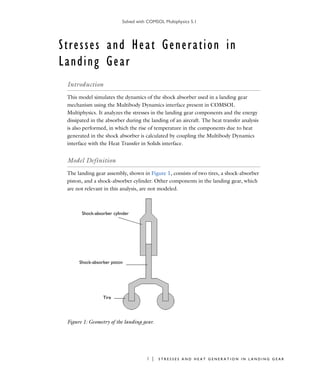
  • 1. Solved with COMSOL Multiphysics 5.1 1 | S T R E S S E S A N D H E A T G E N E R A T I O N I N L A N D I N G G E A R Stresses and Heat Generation in Landing Gear Introduction This model simulates the dynamics of the shock absorber used in a landing gear mechanism using the Multibody Dynamics interface present in COMSOL Multiphysics. It analyzes the stresses in the landing gear components and the energy dissipated in the absorber during the landing of an aircraft. The heat transfer analysis is also performed, in which the rise of temperature in the components due to heat generated in the shock absorber is calculated by coupling the Multibody Dynamics interface with the Heat Transfer in Solids interface. Model Definition The landing gear assembly, shown in Figure 1, consists of two tires, a shock-absorber piston, and a shock-absorber cylinder. Other components in the landing gear, which are not relevant in this analysis, are not modeled. Shock-absorber cylinder Shock-absorber piston Tire Figure 1: Geometry of the landing gear.
  • 2. Solved with COMSOL Multiphysics 5.1 2 | S T R E S S E S A N D H E A T G E N E R A T I O N I N L A N D I N G G E A R The shock-absorber piston and cylinder are connected through a prismatic joint that has only one translational degree of freedom. The joint is loaded with a spring and a damper to absorb the shock during the landing. This is modeled using the spring and damper subnode of the prismatic joint. To model the effect of the tires, the bottom surfaces of the shock-absorber piston are loaded with equivalent spring and damper. The energy dissipated in the damper is used as a heat source on the common boundaries of the shock-absorber piston and cylinder. Remaining boundaries are considered to be insulated. The heat generated on the boundaries is conducted into the landing gear components during the landing, which increases their temperature. Results and Discussion Figure 2 displays the stress generated in the landing gear components at the time when the displacement reaches its maximum. Figure 2: von Mises stress distribution in the deformed landing gear. Figure 3 shows the relative displacement between the shock-absorber piston and cylinder during landing. The amplitude of the relative displacement is very high initially, but it decays rapidly due to the energy loss in the shock absorber and tires.
  • 3. Solved with COMSOL Multiphysics 5.1 3 | S T R E S S E S A N D H E A T G E N E R A T I O N I N L A N D I N G G E A R Figure 3: Relative displacement between the shock-absorber piston and cylinder. Figure 4: Relative velocity between the shock-absorber piston and cylinder.
  • 4. Solved with COMSOL Multiphysics 5.1 4 | S T R E S S E S A N D H E A T G E N E R A T I O N I N L A N D I N G G E A R Figure 4 shows the relative velocity variation between the shock-absorber piston and cylinder during landing. The relative velocity is also very high initially, and it decays to zero due to the energy loss in shock absorber and tires during the course of landing. The force component in y direction in the prismatic joint is shown in Figure 5. The force also decays with time and subsequently acquires a steady state value equivalent to the weight of the whole supported system. Figure 6 shows the variation in the energy components during the landing. Initially, the kinetic energy is very high. But due to the dissipation in the subsequent cycles, it decays to zero. The other forms of energies, such as strain energy and potential energy, are very small as compared to the kinetic energy. This happens because most of the kinetic energy is stored in the shock absorber initially and then dissipated before getting converted to any other forms of energy. The temperature rise in the components due to heat dissipated in shock-absorber is shown in Figure 7. The maximum temperature rise occurs near the piston-cylinder boundaries. Figure 5: The y component of force in the shock-absorber.
  • 5. Solved with COMSOL Multiphysics 5.1 5 | S T R E S S E S A N D H E A T G E N E R A T I O N I N L A N D I N G G E A R Figure 6: Variation of different types of energy in the gear during landing. Figure 7: Temperature profile in the landing gear.
  • 6. Solved with COMSOL Multiphysics 5.1 6 | S T R E S S E S A N D H E A T G E N E R A T I O N I N L A N D I N G G E A R Application Library path: Multibody_Dynamics_Module/ Automotive_and_Aerospace/landing_gear Modeling Instructions From the File menu, choose New. N E W 1 In the New window, click Model Wizard. M O D E L W I Z A R D 1 In the Model Wizard window, click 2D. 2 In the Select physics tree, select Structural Mechanics>Multibody Dynamics (mbd). 3 Click Add. 4 In the Select physics tree, select Heat Transfer>Heat Transfer in Solids (ht). 5 Click Add. 6 Click Study. 7 In the Select study tree, select Preset Studies for Selected Physics Interfaces>Time Dependent. 8 Click Done. G L O B A L D E F I N I T I O N S Parameters 1 On the Home toolbar, click Parameters. 2 In the Settings window for Parameters, locate the Parameters section. 3 In the table, enter the following settings: Name Expression Value Description m 5000[kg] 5000 kg Mass of the aircraft vi 10[m/s] 10 m/s Downward velocity of the aircraft k_sa 2.5e6[N/m] 2.5E6 N/m Spring constant of shock absorber
  • 7. Solved with COMSOL Multiphysics 5.1 7 | S T R E S S E S A N D H E A T G E N E R A T I O N I N L A N D I N G G E A R If you do not want to build all the geometry, you can load the geometry sequence from the stored model. In the Model Builder window, under Component 1 right-click Geometry 1 and choose Insert Sequence from File. Browse to the applicationโ€™s Application Library folder and double-click the file landing_gear.mph. You can then continue to the Add Material section below. To build the geometry from a scratch, continue here. G E O M E T R Y 1 Circle 1 (c1) 1 On the Geometry toolbar, click Primitives and choose Circle. 2 In the Settings window for Circle, locate the Size and Shape section. 3 In the Radius text field, type 0.15. 4 Locate the Position section. In the x text field, type -0.3. Bรฉzier Polygon 1 (b1) 1 On the Geometry toolbar, click Primitives and choose Bรฉzier Polygon. 2 In the Settings window for Bรฉzier Polygon, locate the Polygon Segments section. 3 Find the Added segments subsection. Click Add Linear. 4 Find the Control points subsection. In row 1, set x to -0.35. 5 In row 2, set x to -0.35. 6 In row 2, set y to 0.3. 7 Find the Added segments subsection. Click Add Linear. 8 Find the Control points subsection. In row 2, set x to -0.15. 9 In row 2, set y to 0.4. 10 Find the Added segments subsection. Click Add Linear. 11 Find the Control points subsection. In row 2, set x to -0.05. 12 Find the Added segments subsection. Click Add Linear. c_sa 5e4[N*s/m] 5E4 Nยทs/m Damping coefficient of shock absorber k_t 2.5e7[N/m] 2.5E7 N/m Stiffness of tyre c_t 2.5e6[N*s/m] 2.5E6 Nยทs/m Damping coefficient of tyre d 0.1[m] 0.1 m Out of plane dimension Name Expression Value Description
  • 8. Solved with COMSOL Multiphysics 5.1 8 | S T R E S S E S A N D H E A T G E N E R A T I O N I N L A N D I N G G E A R 13 Find the Control points subsection. In row 2, set y to 1. 14 Find the Added segments subsection. Click Add Linear. 15 Find the Control points subsection. In row 2, set x to 0. 16 Find the Added segments subsection. Click Add Linear. 17 Find the Control points subsection. In row 2, set y to 0.3. 18 Find the Added segments subsection. Click Add Linear. 19 Find the Control points subsection. In row 2, set x to -0.15+0.1*(sqrt(5)-2). 20 Find the Added segments subsection. Click Add Linear. 21 Find the Control points subsection. In row 2, set x to -0.25. 22 In row 2, set y to 0.3-0.05*(sqrt(5)-1). 23 Find the Added segments subsection. Click Add Linear. 24 Find the Control points subsection. In row 2, set y to 0. Bรฉzier Polygon 2 (b2) 1 On the Geometry toolbar, click Primitives and choose Bรฉzier Polygon. 2 In the Settings window for Bรฉzier Polygon, locate the Polygon Segments section. 3 Find the Added segments subsection. Click Add Linear. 4 Find the Control points subsection. In row 1, set x to -0.15. 5 In row 1, set y to 0.8. 6 In row 2, set x to -0.15. 7 In row 2, set y to 1.3+0.1*sqrt(2). 8 Find the Added segments subsection. Click Add Linear. 9 Find the Control points subsection. In row 2, set x to -0.05. 10 In row 2, set y to 1.4+0.1*sqrt(2). 11 Find the Added segments subsection. Click Add Linear. 12 Find the Control points subsection. In row 2, set y to 1.8. 13 Find the Added segments subsection. Click Add Linear. 14 Find the Control points subsection. In row 2, set x to 0. 15 Find the Added segments subsection. Click Add Linear. 16 Find the Control points subsection. In row 2, set y to 1.4. 17 Find the Added segments subsection. Click Add Linear. 18 Find the Control points subsection. In row 2, set x to -0.05.
  • 9. Solved with COMSOL Multiphysics 5.1 9 | S T R E S S E S A N D H E A T G E N E R A T I O N I N L A N D I N G G E A R 19 Find the Added segments subsection. Click Add Linear. 20 Find the Control points subsection. In row 2, set y to 0.8. 21 Right-click Component 1 (comp1)>Geometry 1>Bรฉzier Polygon 2 (b2) and choose Build Selected. 22 Click the button on the Graphics toolbar. 23 Click the Zoom Extents button on the Graphics toolbar. Copy 1 (copy1) 1 On the Geometry toolbar, click Transforms and choose Copy. 2 Select the object b1 only. Difference 1 (dif1) 1 On the Geometry toolbar, click Booleans and Partitions and choose Difference. 2 Select the object c1 only. 3 In the Settings window for Difference, locate the Difference section. 4 Find the Objects to subtract subsection. Select the Active toggle button. 5 Select the object copy1 only. Mirror 1 (mir1) 1 On the Geometry toolbar, click Transforms and choose Mirror. 2 Click in the Graphics window and then press Ctrl+A to select all objects. 3 In the Settings window for Mirror, locate the Input section. 4 Select the Keep input objects check box. Union 1 (uni1) 1 On the Geometry toolbar, click Booleans and Partitions and choose Union. 2 Select the objects b1 and mir1(1) only. 3 In the Settings window for Union, locate the Union section. 4 Clear the Keep interior boundaries check box. Union 2 (uni2) 1 On the Geometry toolbar, click Booleans and Partitions and choose Union. 2 Select the objects mir1(2) and b2 only. 3 In the Settings window for Union, locate the Union section. 4 Clear the Keep interior boundaries check box.
  • 10. Solved with COMSOL Multiphysics 5.1 10 | S T R E S S E S A N D H E A T G E N E R A T I O N I N L A N D I N G G E A R Union 3 (uni3) 1 On the Geometry toolbar, click Booleans and Partitions and choose Union. 2 Select the objects uni1, mir1(3), and dif1 only. Form Union (fin) 1 In the Model Builder window, under Component 1 (comp1)>Geometry 1 click Form Union (fin). 2 In the Settings window for Form Union/Assembly, locate the Form Union/Assembly section. 3 From the Action list, choose Form an assembly. 4 Right-click Component 1 (comp1)>Geometry 1>Form Union (fin) and choose Build Selected. 5 Click the Go to Default 3D View button on the Graphics toolbar. 6 Click the Zoom Extents button on the Graphics toolbar. A D D M A T E R I A L 1 On the Home toolbar, click Add Material to open the Add Material window. 2 Go to the Add Material window. 3 In the tree, select Built-In>Structural steel. 4 Click Add to Component in the window toolbar. 5 On the Home toolbar, click Add Material to close the Add Material window. M U L T I B O D Y D Y N A M I C S ( M B D ) 1 In the Model Builder window, under Component 1 (comp1) click Multibody Dynamics (mbd). 2 In the Settings window for Multibody Dynamics, locate the Thickness section. 3 In the d text field, type d. Initial Values 1 1 In the Model Builder window, under Component 1 (comp1)>Multibody Dynamics (mbd) click Initial Values 1. 2 In the Settings window for Initial Values, locate the Initial Values section. 3 From the list, choose Locally defined.
  • 11. Solved with COMSOL Multiphysics 5.1 11 | S T R E S S E S A N D H E A T G E N E R A T I O N I N L A N D I N G G E A R 4 Specify the โˆ‚u/โˆ‚t vector as Attachment 1 1 On the Physics toolbar, click Boundaries and choose Attachment. 2 Select Boundaries 34 and 40 only. Attachment 2 1 On the Physics toolbar, click Boundaries and choose Attachment. 2 Select Boundaries 10 and 14 only. Prismatic Joint 1 1 On the Physics toolbar, click Global and choose Prismatic Joint. 2 In the Settings window for Prismatic Joint, locate the Attachment Selection section. 3 From the Source list, choose Attachment 1. 4 From the Destination list, choose Attachment 2. 5 Locate the Axis of Joint section. Specify the e0 vector as Spring and Damper 1 1 On the Physics toolbar, click Attributes and choose Spring and Damper. 2 In the Settings window for Spring and Damper, locate the Spring and Damper: Translational section. 3 In the ku text field, type k_sa. 4 In the cu text field, type c_sa. Use the Added Mass node to account for the mass of the aircraft. Added Mass 1 1 On the Physics toolbar, click Boundaries and choose Added Mass. 2 Select Boundaries 37 and 39 only. 3 In the Settings window for Added Mass, locate the Added Mass section. 4 From the Mass type list, choose Total mass. 0 X -vi Y 0 x -1 y
  • 12. Solved with COMSOL Multiphysics 5.1 12 | S T R E S S E S A N D H E A T G E N E R A T I O N I N L A N D I N G G E A R 5 Specify the m vector as Gravity 1 1 On the Physics toolbar, click Domains and choose Gravity. 2 In the Settings window for Gravity, locate the Domain Selection section. 3 From the Selection list, choose All domains. The Spring Foundation node is used to account for the elastic and damping effects of the tyres. Spring Foundation 1 1 On the Physics toolbar, click Boundaries and choose Spring Foundation. 2 Select Boundaries 2 and 19 only. 3 In the Settings window for Spring Foundation, locate the Spring section. 4 From the Spring type list, choose Total spring constant. 5 From the list, choose Diagonal. 6 In the ktot table, enter the following settings: 7 Click to expand the Viscous damping section. Locate the Viscous Damping section. From the Damping type list, choose Total damping constant. 8 From the list, choose Diagonal. 9 In the dtot table, enter the following settings: D E F I N I T I O N S Integration 1 (intop1) 1 On the Definitions toolbar, click Component Couplings and choose Integration. 2 In the Settings window for Integration, locate the Source Selection section. 3 From the Geometric entity level list, choose Boundary. 0 X m Y 0 0 0 k_t 0 0 0 c_t
  • 13. Solved with COMSOL Multiphysics 5.1 13 | S T R E S S E S A N D H E A T G E N E R A T I O N I N L A N D I N G G E A R 4 Select Boundaries 10 and 14 only. Integration 2 (intop2) 1 On the Definitions toolbar, click Component Couplings and choose Integration. 2 In the Settings window for Integration, locate the Source Selection section. 3 From the Selection list, choose All domains. Variables 1 1 On the Definitions toolbar, click Local Variables. The heat generated due to the energy dissipation in the absorber is modeled as a heat source. This heat source is distributed on the common boundaries of the shock-absorber piston and cylinder. 2 In the Settings window for Variables, locate the Variables section. 3 In the table, enter the following settings: H E A T TR A N S F E R I N S O L I D S ( H T ) Pair Boundary Heat Source 1 1 On the Physics toolbar, in the Boundary section, click Pairs and choose Pair Boundary Heat Source. 2 In the Settings window for Pair Boundary Heat Source, locate the Pair Selection section. 3 In the Pairs list, select Identity Pair 1 (ap1). 4 Locate the Boundary Heat Source section. Click the Overall heat transfer rate button. 5 In the Pb text field, type Q*1[m]/d. Here, the total power is scaled with the actual out-of-plane thickness to get the correct temperature distribution. Name Expression Unit Description Q mbd.prj1.Qdamper W Heat generated per second Wp intop2(mbd.rho*g_const*v*mbd.d) J Potential energy h_sa timeint(0,t,Q) J Energy loss in shock-absorber Ws_sa mbd.prj1.Wspring J Energy stored in shock-absorber
  • 14. Solved with COMSOL Multiphysics 5.1 14 | S T R E S S E S A N D H E A T G E N E R A T I O N I N L A N D I N G G E A R M E S H 1 1 In the Model Builder window, under Component 1 (comp1) click Mesh 1. 2 In the Settings window for Mesh, locate the Mesh Settings section. 3 From the Element size list, choose Finer. 4 Click the Build All button. S T U D Y 1 Step 1: Time Dependent 1 In the Model Builder window, under Study 1 click Step 1: Time Dependent. 2 In the Settings window for Time Dependent, locate the Study Settings section. 3 In the Times text field, type range(0,0.01,0.7). 4 On the Home toolbar, click Compute. R E S U L T S Displacement (mbd) Follow these instructions to generate a plot similar to that is shown in Figure 2: 1 In the Model Builder window, click Displacement (mbd). 2 In the Settings window for 2D Plot Group, type Stress in the Label text field. 3 Locate the Plot Settings section. From the Frame list, choose Material (X, Y, Z). 4 Locate the Data section. From the Time (s) list, choose 0.06. Stress 1 In the Model Builder window, expand the Results>Stress node, then click Surface 1. 2 In the Settings window for Surface, click Replace Expression in the upper-right corner of the Expression section. From the menu, choose Component 1>Multibody Dynamics>Stress>mbd.mises - von Mises stress. 3 Click to expand the Quality section. From the Resolution list, choose No refinement. 4 On the Stress toolbar, click Plot. 5 Click the Zoom Extents button on the Graphics toolbar. Follow these instructions to generate a plot similar to that is shown in Figure 7: Temperature (ht) 1 In the Model Builder window, expand the Results>Temperature (ht) node, then click Surface 1.
  • 15. Solved with COMSOL Multiphysics 5.1 15 | S T R E S S E S A N D H E A T G E N E R A T I O N I N L A N D I N G G E A R 2 In the Settings window for Surface, locate the Quality section. 3 From the Resolution list, choose No refinement. 4 Right-click Results>Temperature (ht)>Surface 1 and choose Deformation. 5 In the Settings window for Deformation, locate the Scale section. 6 Select the Scale factor check box. 7 In the associated text field, type 1. 8 On the Temperature (ht) toolbar, click Plot. Follow these instructions to generate a relative displacement plot similar to that is shown in Figure 3: 1D Plot Group 5 1 On the Home toolbar, click Add Plot Group and choose 1D Plot Group. 2 In the Settings window for 1D Plot Group, type Relative displacement in the Label text field. 3 Click to expand the Title section. From the Title type list, choose None. Relative displacement 1 On the Relative displacement toolbar, click Global. 2 In the Settings window for Global, click Replace Expression in the upper-right corner of the y-axis data section. From the menu, choose Component 1>Multibody Dynamics>Prismatic joints>Prismatic Joint 1>mbd.prj1.u - Relative displacement. 3 Click to expand the Legends section. Clear the Show legends check box. 4 Click to expand the Coloring and style section. Locate the Coloring and Style section. Find the Line style subsection. In the Width text field, type 2. 5 On the Relative displacement toolbar, click Plot. Follow these instructions to generate a relative velocity plot similar to that is shown in Figure 4: Relative displacement 1 1 In the Model Builder window, right-click Relative displacement and choose Duplicate. 2 In the Settings window for 1D Plot Group, type Relative velocity in the Label text field. Relative velocity 1 In the Model Builder window, expand the Results>Relative velocity node, then click Global 1.
  • 16. Solved with COMSOL Multiphysics 5.1 16 | S T R E S S E S A N D H E A T G E N E R A T I O N I N L A N D I N G G E A R 2 In the Settings window for Global, click Replace Expression in the upper-right corner of the y-axis data section. From the menu, choose Component 1>Multibody Dynamics>Prismatic joints>Prismatic Joint 1>mbd.prj1.u_t - Relative velocity. 3 On the Relative velocity toolbar, click Plot. Follow these instructions to generate a joint force plot similar to that is shown in Figure 5: Relative velocity 1 1 In the Model Builder window, right-click Relative velocity and choose Duplicate. 2 In the Settings window for 1D Plot Group, type Joint Force in the Label text field. Joint Force 1 In the Model Builder window, expand the Results>Joint Force node, then click Global 1. 2 In the Settings window for Global, click Replace Expression in the upper-right corner of the y-axis data section. From the menu, choose Component 1>Multibody Dynamics>Prismatic joints>Prismatic Joint 1>Joint force>mbd.prj1.Fy - Joint force, y component. 3 On the Joint Force toolbar, click Plot. To generate energy plot shown in Figure 6, follow the instructions below. 1D Plot Group 8 1 On the Home toolbar, click Add Plot Group and choose 1D Plot Group. 2 In the Settings window for 1D Plot Group, type Energy in the Label text field. 3 Locate the Title section. From the Title type list, choose None. Energy 1 On the Energy toolbar, click Global. 2 In the Settings window for Global, click Replace Expression in the upper-right corner of the y-axis data section. From the menu, choose Component 1>Definitions>Variables>Wp - Potential energy. 3 Click Add Expression in the upper-right corner of the y-axis data section. From the menu, choose Component 1>Multibody Dynamics>Global>mbd.Wk_tot - Total kinetic energy. 4 Click Add Expression in the upper-right corner of the y-axis data section. From the menu, choose Component 1>Multibody Dynamics>Global>mbd.Ws_tot - Total elastic strain energy.
  • 17. Solved with COMSOL Multiphysics 5.1 17 | S T R E S S E S A N D H E A T G E N E R A T I O N I N L A N D I N G G E A R 5 Click Add Expression in the upper-right corner of the y-axis data section. From the menu, choose Component 1>Definitions>Variables>h_sa - Energy loss in shock-absorber. 6 Click Add Expression in the upper-right corner of the y-axis data section. From the menu, choose Component 1>Definitions>Variables>Ws_sa - Energy stored in shock-absorber. 7 Locate the Coloring and Style section. Find the Line style subsection. In the Width text field, type 2. 8 Find the Line markers subsection. From the Marker list, choose Cycle. 9 On the Energy toolbar, click Plot. 10 In the Model Builder window, click Energy. 11 In the Settings window for 1D Plot Group, locate the Plot Settings section. 12 Select the y-axis label check box. 13 In the associated text field, type Energy (J). 14 Click to expand the Axis section. Select the Manual axis limits check box. 15 In the y maximum text field, type 3.1e5. 16 On the Energy toolbar, click Plot. Use the instructions below to generate an animation of the stress distribution in the landing gear components. Export 1 On the Results toolbar, click Animation and choose Animation. 2 In the Settings window for Animation, locate the Target section. 3 From the Target list, choose Player. 4 Locate the Frames section. In the Number of frames text field, type 100. 5 Right-click Results>Export>Animation 1 and choose Play. Finally, follow these instructions to generate an animation of the temperature distribution in the components. 6 On the Results toolbar, click Animation and choose Animation. 7 In the Settings window for Animation, locate the Target section. 8 From the Target list, choose Player. 9 Locate the Scene section. From the Subject list, choose Temperature (ht). 10 Locate the Frames section. In the Number of frames text field, type 100.
  • 18. Solved with COMSOL Multiphysics 5.1 18 | S T R E S S E S A N D H E A T G E N E R A T I O N I N L A N D I N G G E A R 11 Right-click Results>Export>Animation 2 and choose Play.