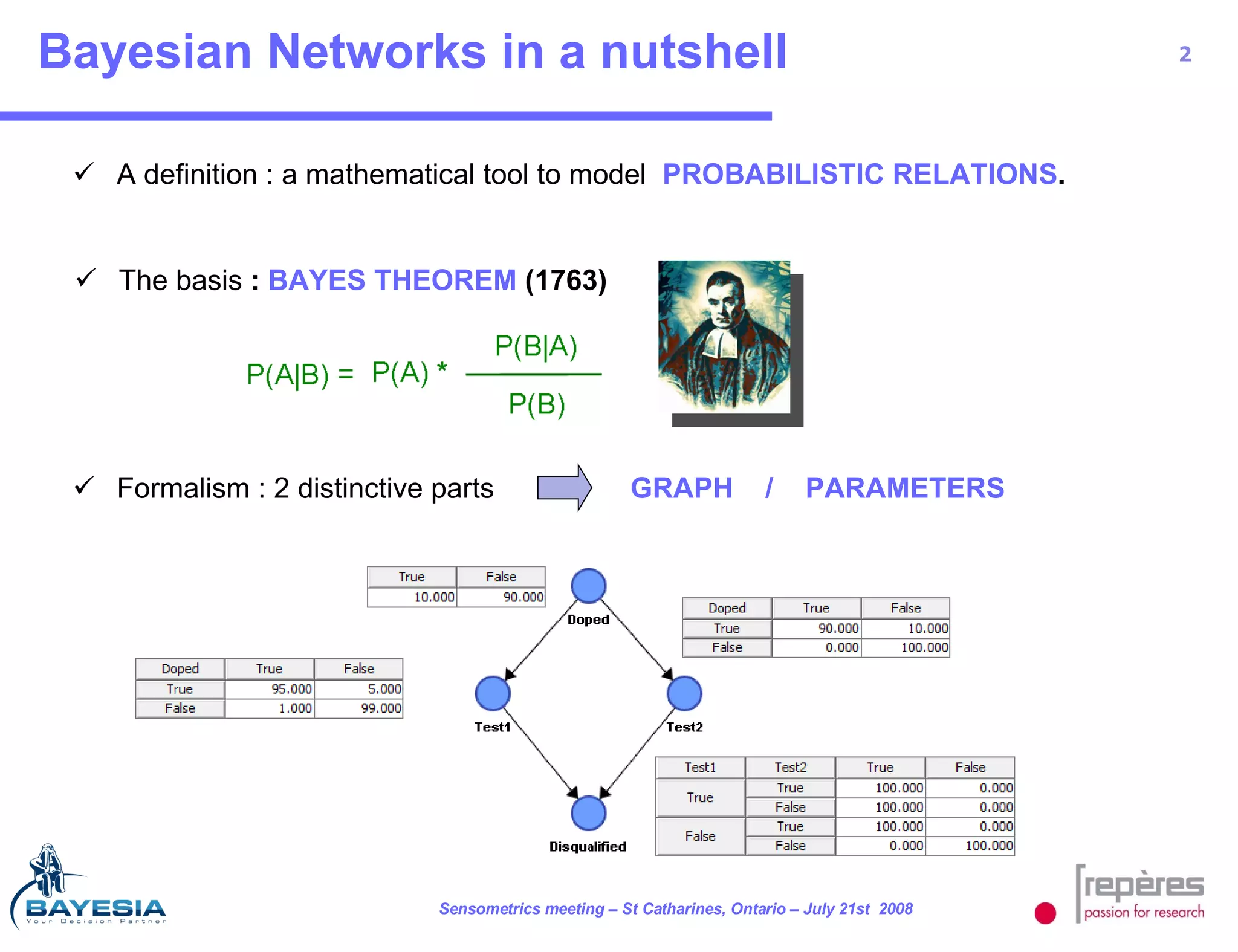
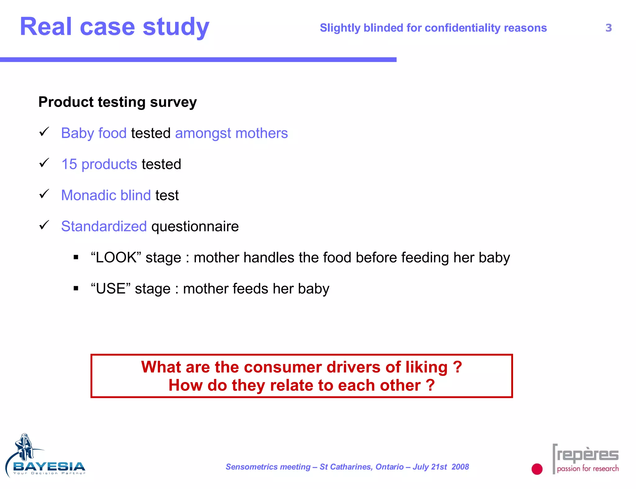
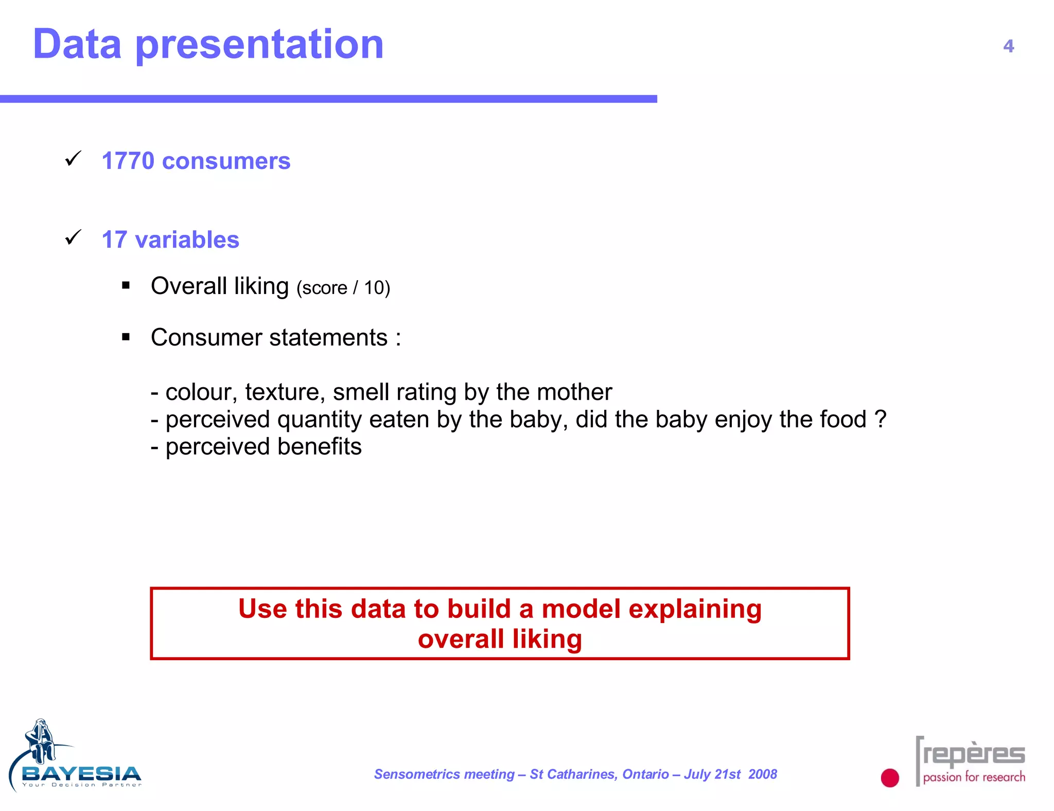
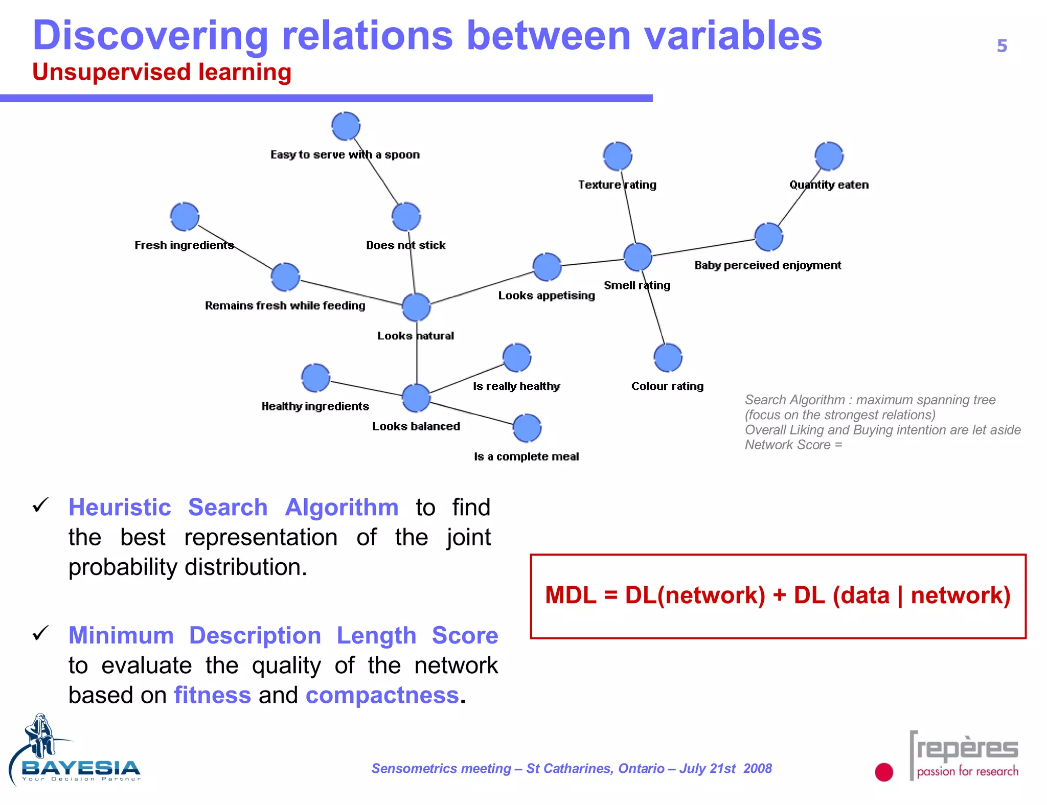
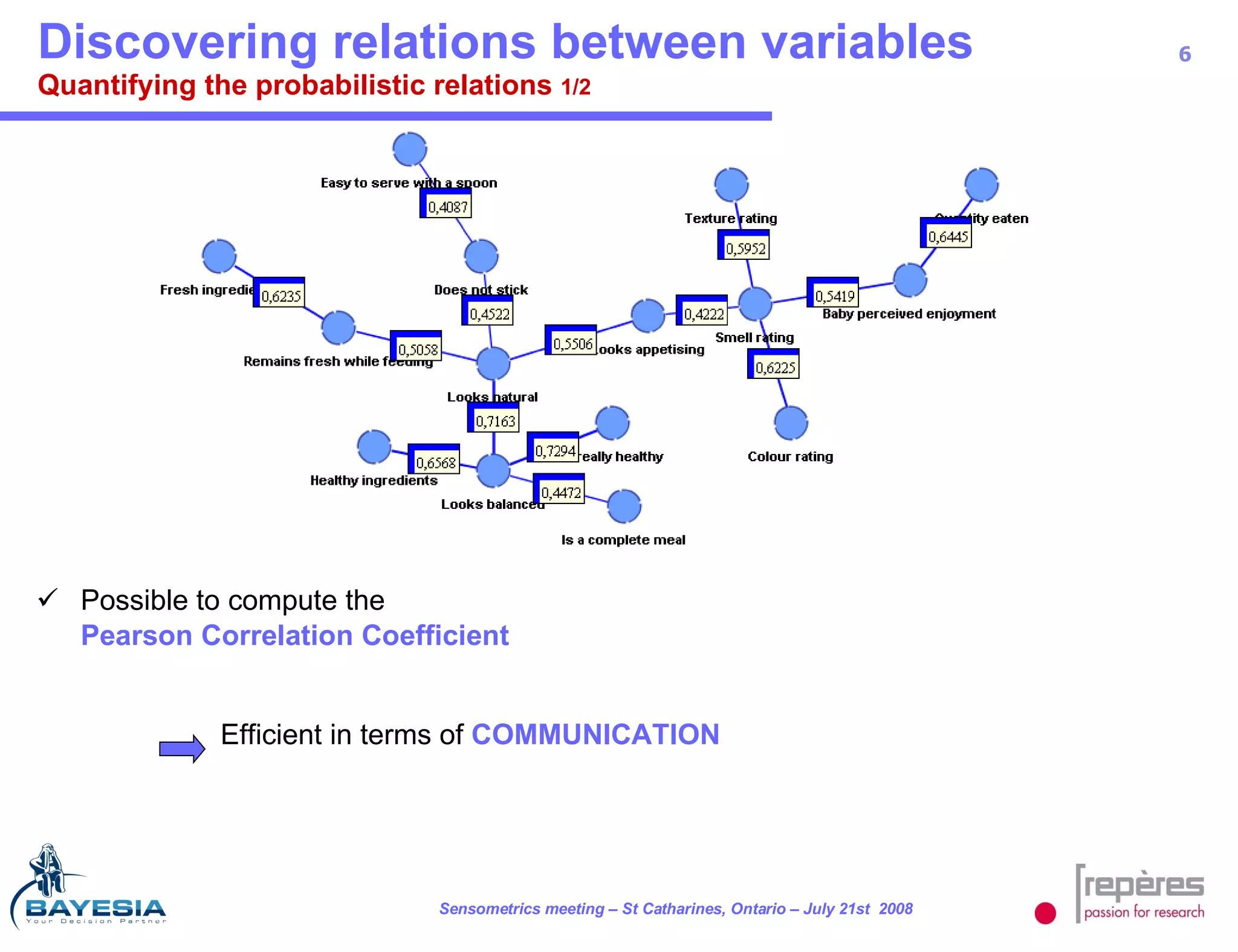
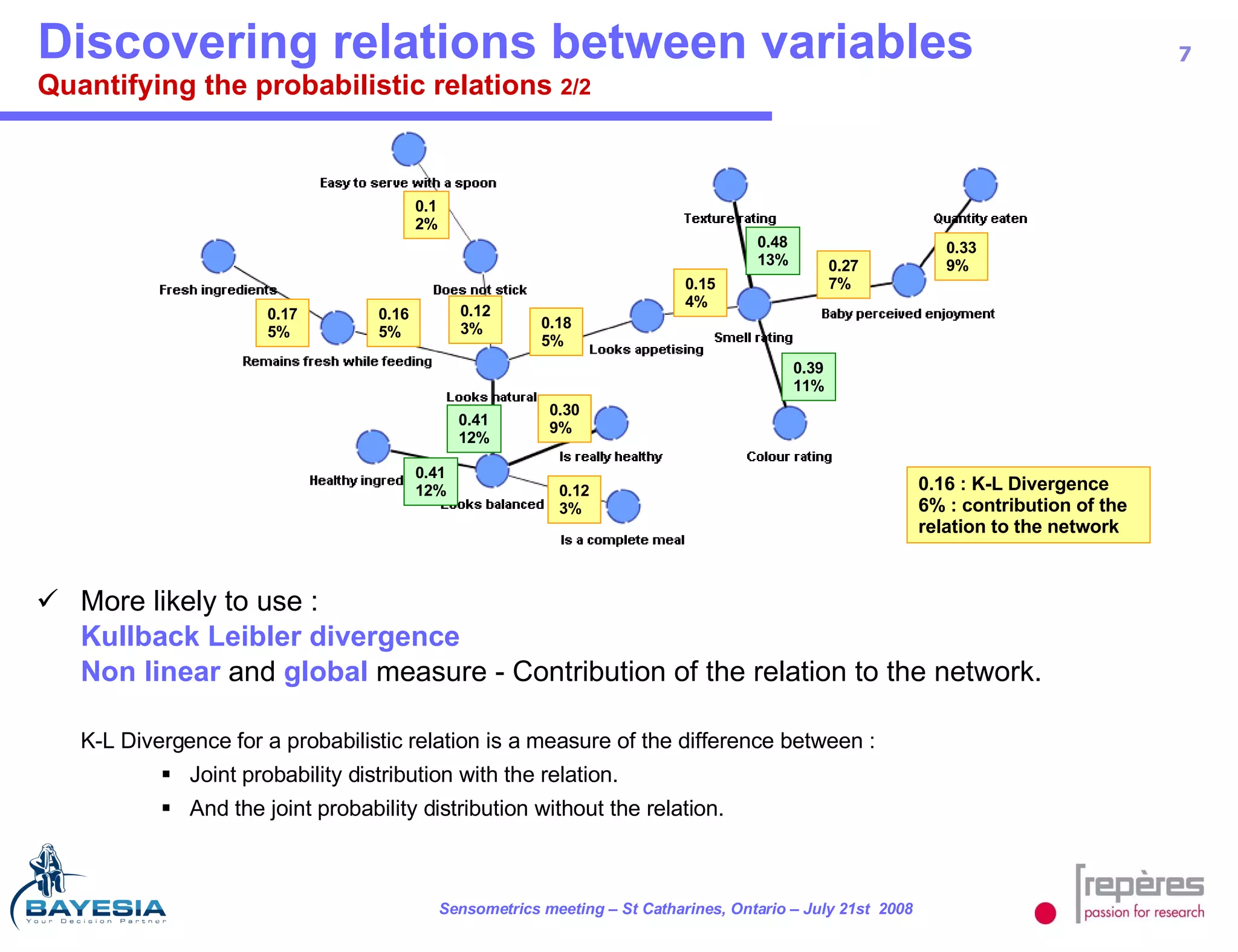
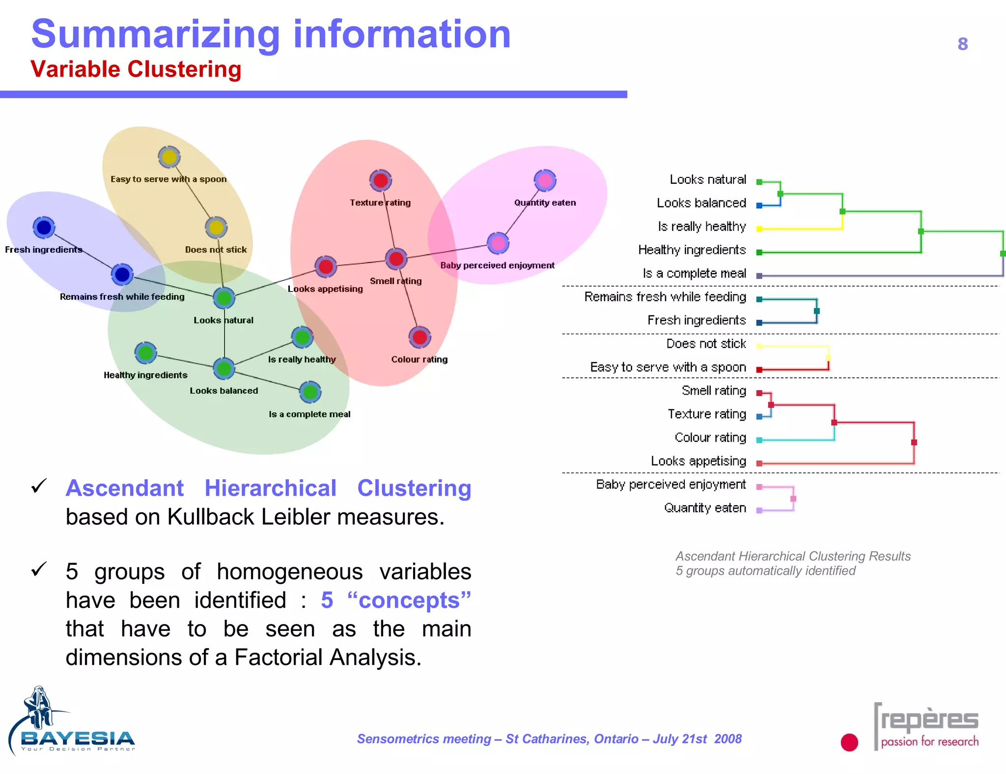
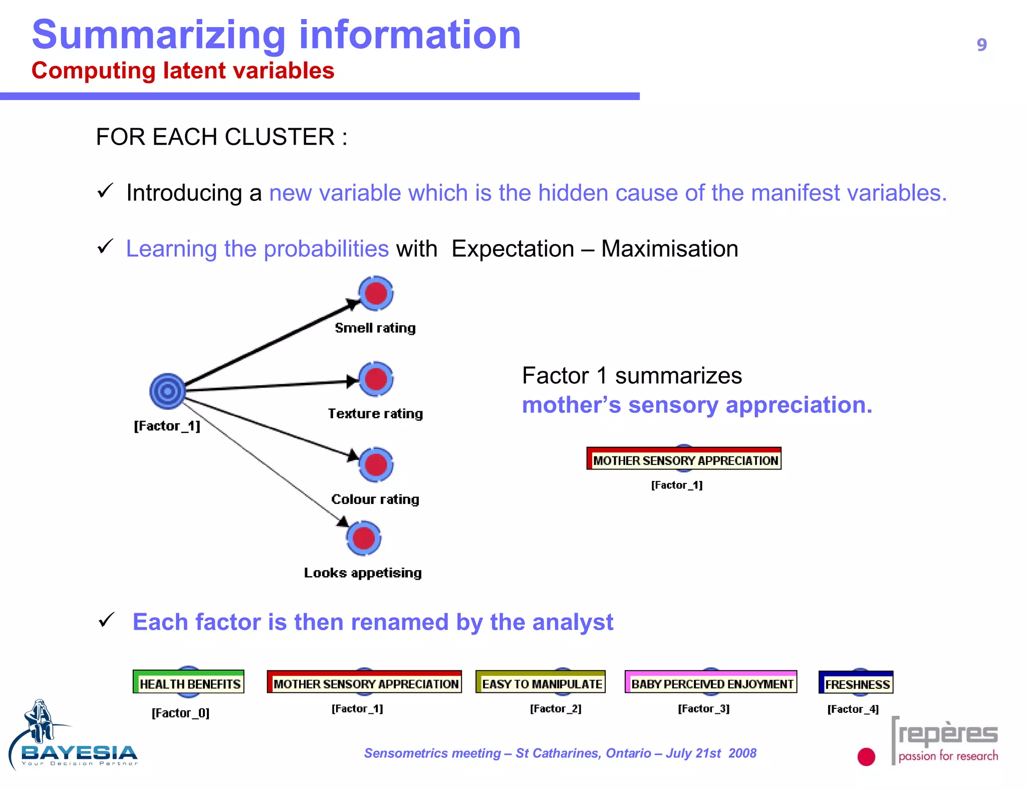
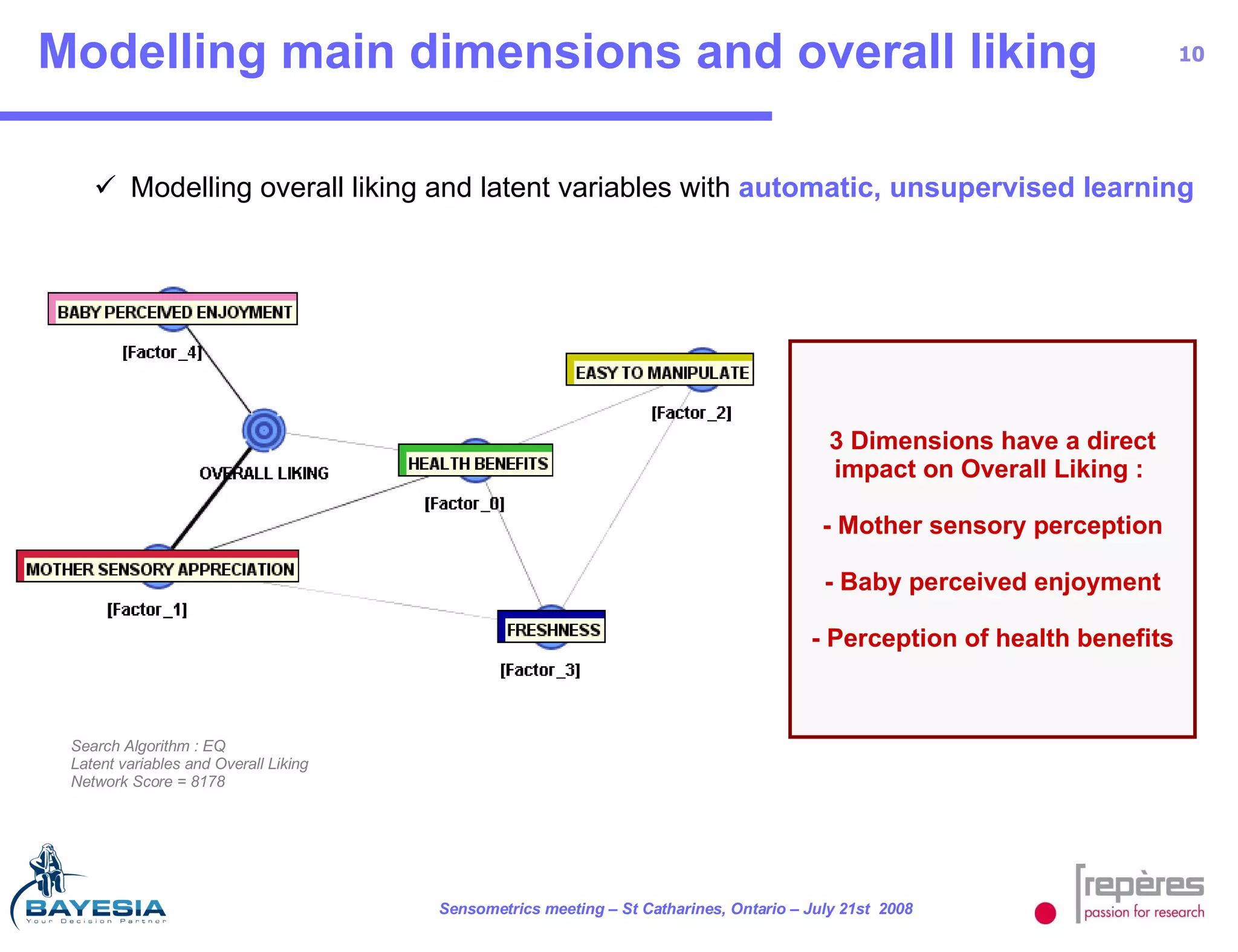
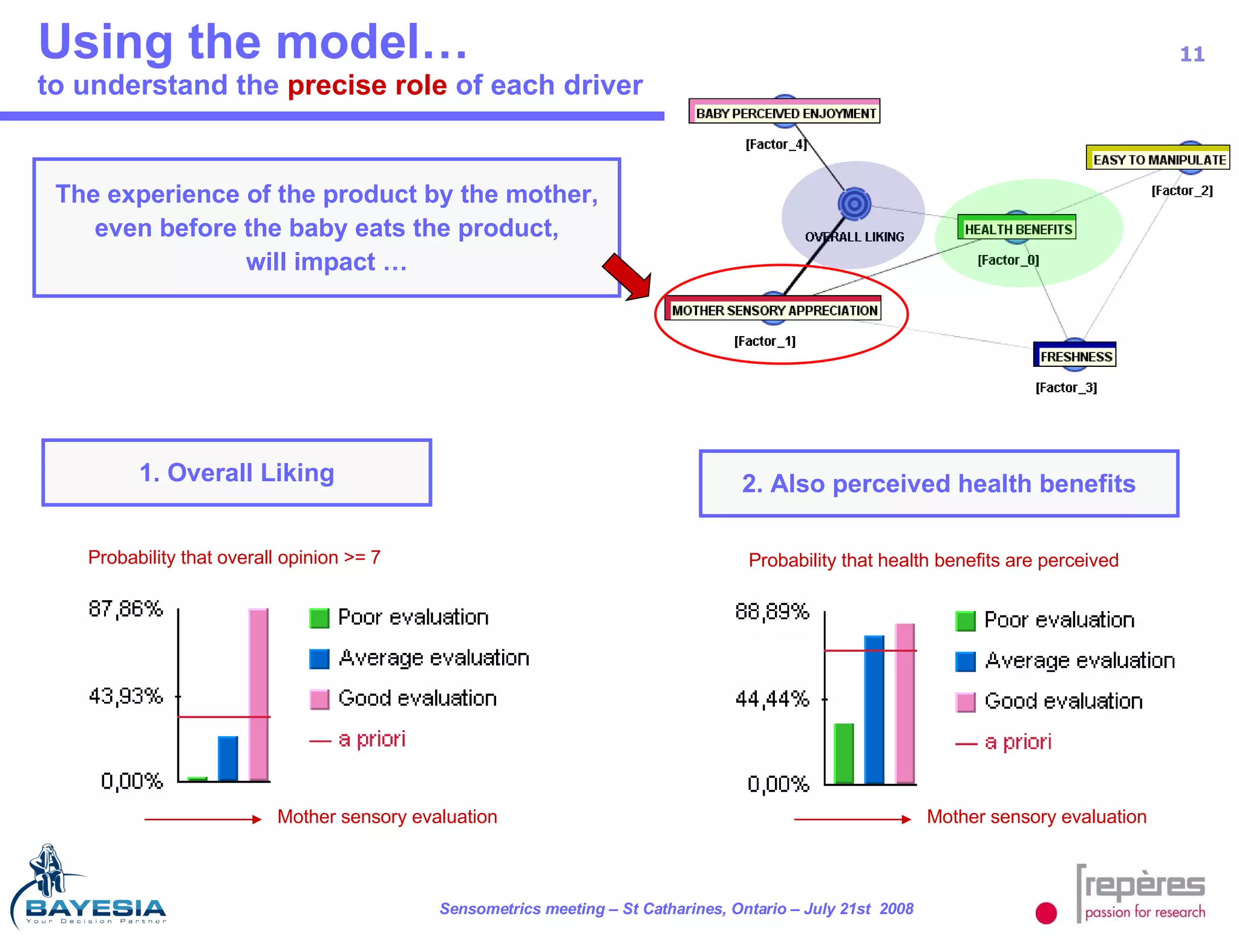
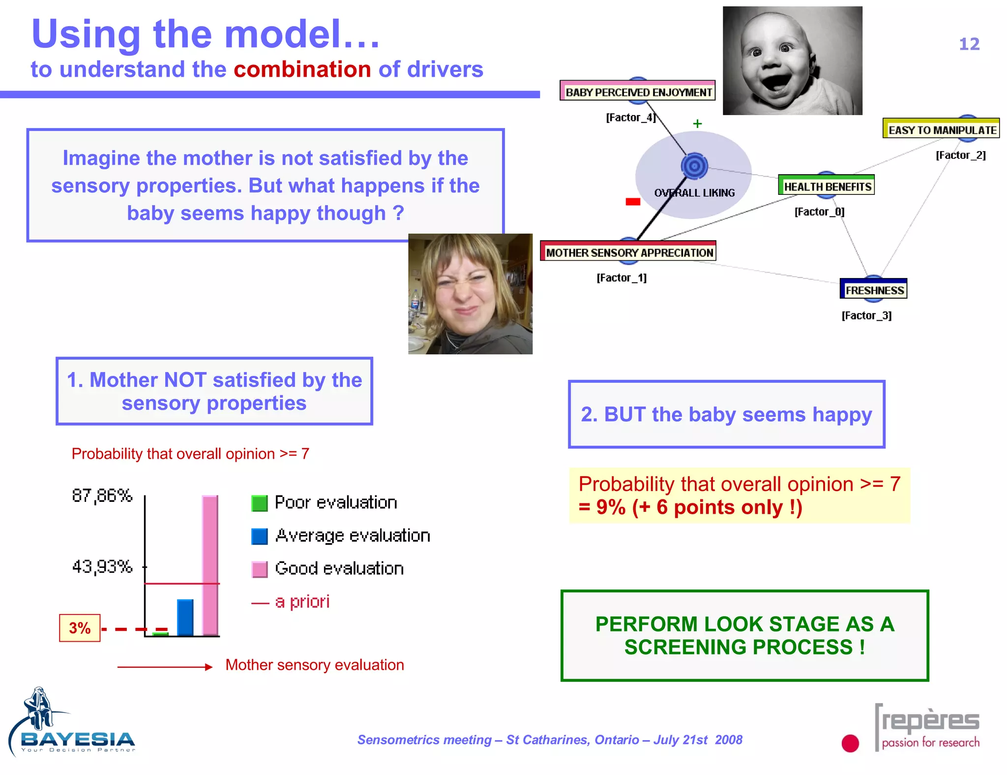
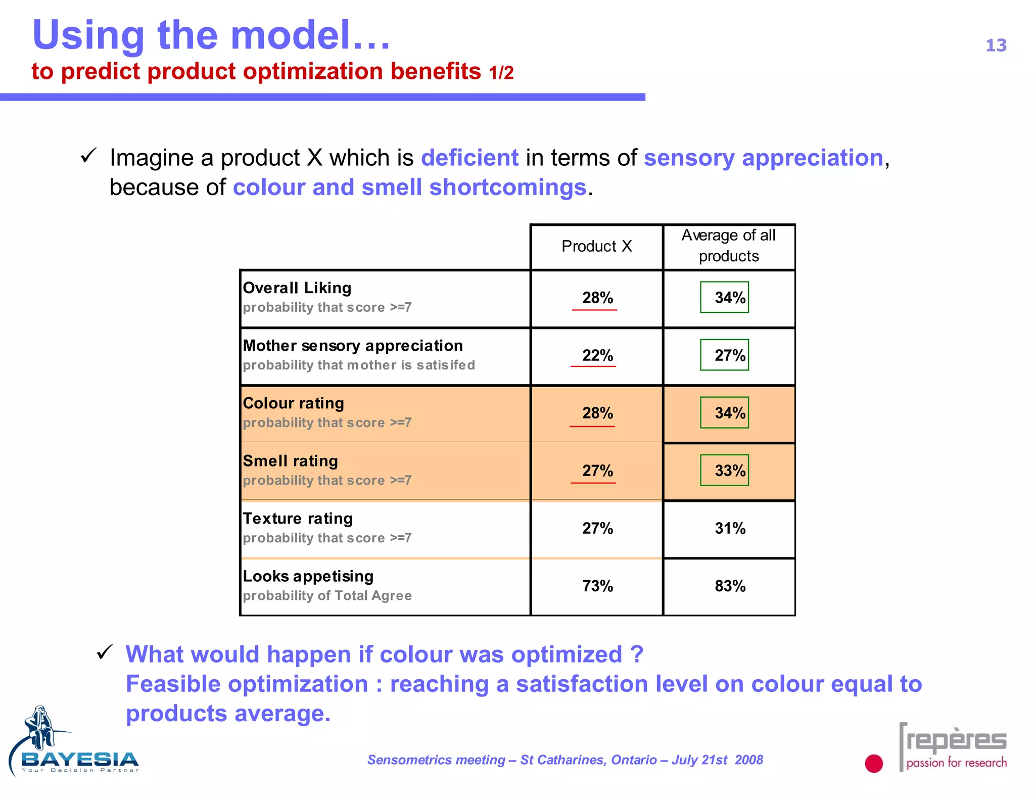
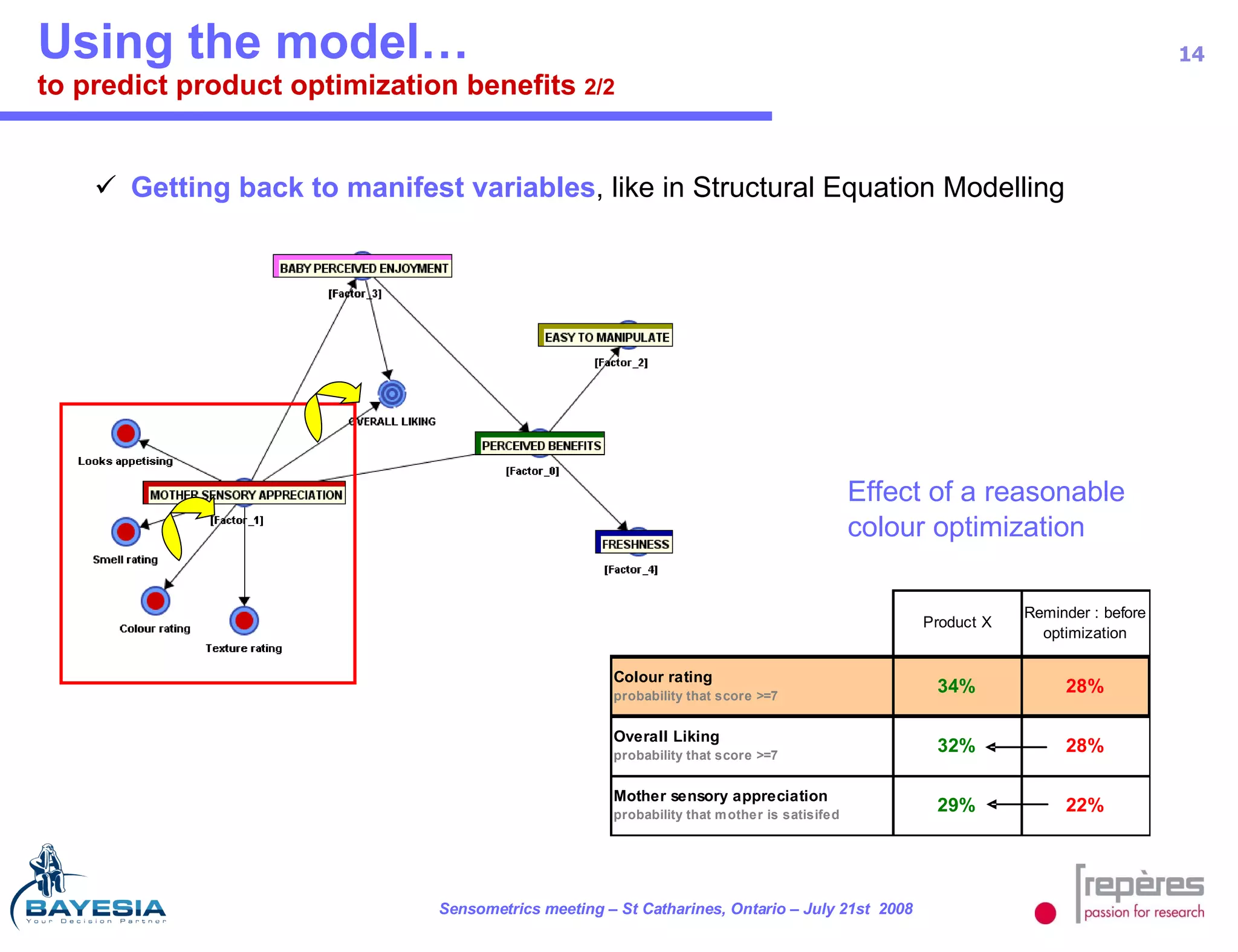
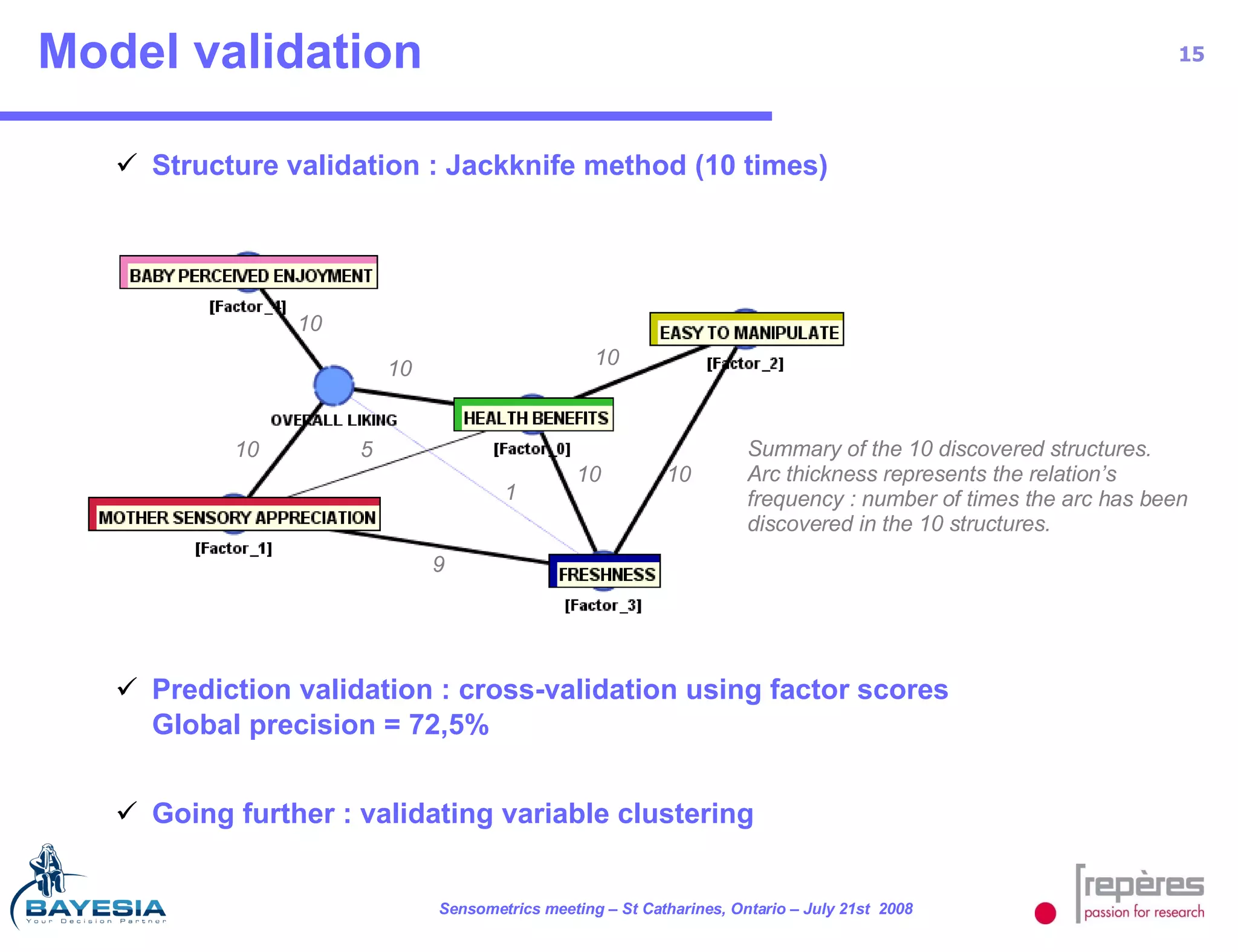
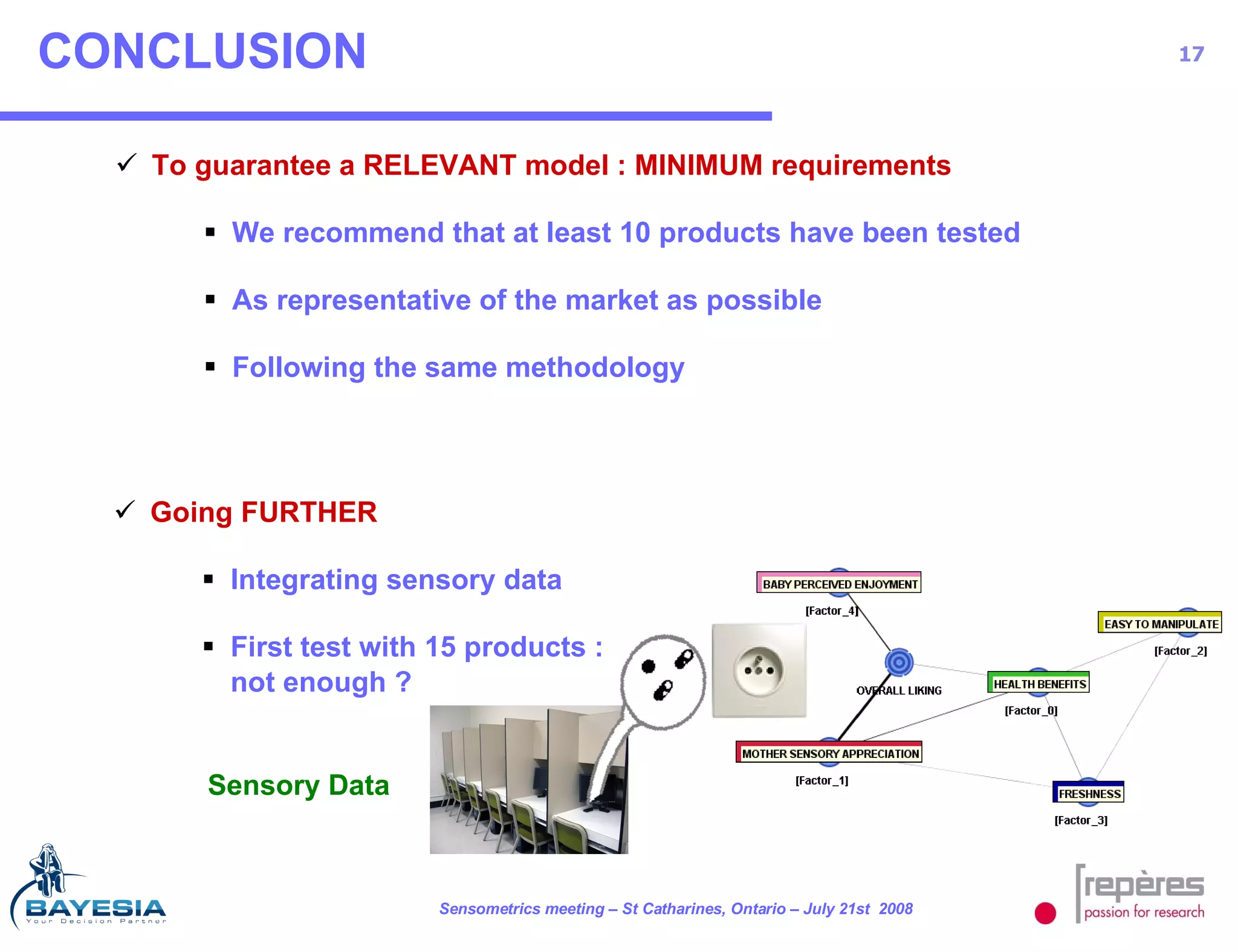
The document summarizes a study that used Bayesian networks to understand the consumer drivers of liking for baby food products. It analyzed survey data from 1770 mothers who tested 15 baby food products. The Bayesian network identified 5 key consumer dimensions that impact overall liking: 1) mother's sensory perception, 2) baby's perceived enjoyment, and 3) perception of health benefits. The model found that a mother's sensory evaluation, even before feeding the baby, impacts overall liking. Optimizing aspects like color could significantly increase the likelihood that mothers rate products positively. Validation tests confirmed the model's ability to understand and predict consumer behavior.

1. Studying consumer drivers with Bayesian Networks Sensometrics meeting – St Catharines, Ontario – July 21st 2008

2. Bayesian Networks in a nutshell A definition : a mathematical tool to model PROBABILISTIC RELATIONS . The basis : BAYES THEOREM (1763) Formalism : 2 distinctive parts GRAPH / PARAMETERS

3. Real case study Slightly blinded for confidentiality reasons Product testing survey Baby food tested amongst mothers 15 products tested Monadic blind test Standardized questionnaire “ LOOK” stage : mother handles the food before feeding her baby “ USE” stage : mother feeds her baby What are the consumer drivers of liking ? How do they relate to each other ?

4. Data presentation 1770 consumers 17 variables Overall liking (score / 10) Consumer statements : - colour, texture, smell rating by the mother - perceived quantity eaten by the baby, did the baby enjoy the food ? - perceived benefits Use this data to build a model explaining overall liking

5. Heuristic Search Algorithm to find the best representation of the joint probability distribution. Discovering relations between variables Unsupervised learning Minimum Description Length Score to evaluate the quality of the network based on fitness and compactness . MDL = DL(network) + DL (data | network) Search Algorithm : maximum spanning tree (focus on the strongest relations) Overall Liking and Buying intention are let aside Network Score =

6. Discovering relations between variables Quantifying the probabilistic relations 1/2 Possible to compute the Pearson Correlation Coefficient Efficient in terms of COMMUNICATION

7. 0.41 12% 0.30 9% 0.12 3% 0.48 13% 0.18 5% 0.1 2% 0.39 11% 0.27 7% 0.33 9% 0.16 5% 0.17 5% 0.15 4% 0.16 : K-L Divergence 6% : contribution of the relation to the network More likely to use : Kullback Leibler divergence Non linear and global measure - Contribution of the relation to the network. K-L Divergence for a probabilistic relation is a measure of the difference between : Joint probability distribution with the relation. And the joint probability distribution without the relation. 0.12 3% 0.41 12% Discovering relations between variables Quantifying the probabilistic relations 2/2

8. Summarizing information Variable Clustering Ascendant Hierarchical Clustering based on Kullback Leibler measures. 5 groups of homogeneous variables have been identified : 5 “concepts” that have to be seen as the main dimensions of a Factorial Analysis. Ascendant Hierarchical Clustering Results 5 groups automatically identified

9. FOR EACH CLUSTER : Introducing a new variable which is the hidden cause of the manifest variables. Learning the probabilities with Expectation – Maximisation Summarizing information Computing latent variables Each factor is then renamed by the analyst Factor 1 summarizes mother’s sensory appreciation.

10. Modelling main dimensions and overall liking Modelling overall liking and latent variables with automatic, unsupervised learning 3 Dimensions have a direct impact on Overall Liking : - Mother sensory perception - Baby perceived enjoyment - Perception of health benefits Search Algorithm : EQ Latent variables and Overall Liking Network Score = 8178

11. Using the model… to understand the precise role of each driver The experience of the product by the mother, even before the baby eats the product, will impact … Mother sensory evaluation Probability that overall opinion >= 7 1. Overall Liking Probability that health benefits are perceived 2. Also perceived health benefits Mother sensory evaluation

12. Using the model… to understand the combination of drivers PERFORM LOOK STAGE AS A SCREENING PROCESS ! Imagine the mother is not satisfied by the sensory properties. But what happens if the baby seems happy though ? 2. BUT the baby seems happy Probability that overall opinion >= 7 = 9% (+ 6 points only !) + 1. Mother NOT satisfied by the sensory properties - 3% Mother sensory evaluation Probability that overall opinion >= 7

13. Using the model… to predict product optimization benefits 1/2 What would happen if colour was optimized ? Feasible optimization : reaching a satisfaction level on colour equal to products average. Imagine a product X which is deficient in terms of sensory appreciation , because of colour and smell shortcomings .

14. Using the model… to predict product optimization benefits 2/2 Getting back to manifest variables , like in Structural Equation Modelling Effect of a reasonable colour optimization

15. Model validation Structure validation : Jackknife method (10 times) Prediction validation : cross-validation using factor scores Global precision = 72,5% Summary of the 10 discovered structures. Arc thickness represents the relation’s frequency : number of times the arc has been discovered in the 10 structures. 10 10 10 9 10 10 10 5 Going further : validating variable clustering 1

16. CONCLUSION Good tool to UNDERSTAND and PREDICT (Diagnosis and Simulation) How consumer dimensions impact Liking How consumer dimensions relate to each other Product optimization effects SOUND and TRANSPARENT computations Everything relates to conditional probabilities Stable structures validated by Jackknife validation : no over fitting (conservative learning) Good COMMUNICATION tool Graphical representation Probabilities are easy to understand

17. CONCLUSION To guarantee a RELEVANT model : MINIMUM requirements We recommend that at least 10 products have been tested As representative of the market as possible Following the same methodology Going FURTHER Integrating sensory data First test with 15 products : not enough ? Sensory Data

18. THANK YOU FOR YOUR ATTENTION ! Jouffe Lionel Managing Director [email_address] Craignou Fabien Data Mining Department Manager [email_address]