MARKETING STRATEGY
EXOHIND - HIGHLIGHTS
Presented by
Soumyadeep Chowdhury
EXOHIND GROWTH PLAN – EXTENDED BDM
• ‘ExoHind’ is a start-up company that is funded partly
by seed capital of the founding members and partly by
taking loan and going to start a business in the
Lifestyle travel category
• Since this is a start-up so I don’t have any sales data
for it
• In order to forecast our sales I used Brand level
extension of Bass Diffusion Model –
• Then we use the Funds Balance Equation to identify
the expected growth rate
Year 1 Year 2 Year 3
Revenue 21576742 22929742 24282742
Growth Rate 0 6.27 5.90
Expenses 5000000 5000000 5000000
Profit 16576742 17929742 19282742
RONA 2.81 3.04 3.27
debt/equity 0.50 1.50 2.00
retained earning ratio r 0.77 0.78 0.79
g(s) 3.20 5.82 7.79
BRAND ATTRIBUTES & IMPORTANCE - FISHBEIN
• We use the reverse fishbein model to find
out the relative importance of the three
attributes that are relevant for us
• We found the rough estimates of market
shares of the various competitors for
previous year
• For this year we use Bass Diffusion model
to forecast category level sales and
calculate market share
• From that market share we find out attitude
and then run a Regression analysis on
Brand Attitudes and beliefs to find out the
‘Importance’ ratings
Attributes
MakemyT
rip Yatra ExoHind Others
Importan
ce
Arts & Cultural value 7 6 9 8 b1 = 5
Website quality 7 6 8 7 b2 = 14
Travel experience in
India 9 8 7 8 b3 = 81
Attitude
A1 =
10.58
A2 =
5.29
A3 =
2.47 A4 = 6.17 100
Market Share 0.432 0.216 0.101 0.252 1.000
CLASSIFICATION AND REGRESSION TREE
SEGMENTATION
• Here I have taken a representative data set of
customers, based on various demographic
and psychographic attributes
• Then I use CART algorithm on that data set
• This algorithm basically divides the records in
the data set into various decision nodes
based on the criterion mentioned in the
candidate split
• Each split gives us a set of nodes
• We measure ‘Φ’ – the goodness of split for
each candidate splits
• Φ(s|t) = 2 PLPR 𝑗
# 𝐶𝑙𝑎𝑠𝑠𝑒𝑠
| 𝑃 𝑗 𝑡 𝐿 − 𝑃(𝑗|𝑡 𝑅)|
• The split with highest ‘Φ’ value gives us the
desired segment
Custom
er Income Age Internet
Museum
Attendance
Travel to
India
ExoHind
Prospect
1 30k 20-30 No Yes No No
2 50k 30-40 Yes No Yes No
3 80k 50+ Yes Yes Yes Yes
4 30k 20-30 Yes No No No
5 45k 30-40 Yes No Yes No
6 55k 30-40 Yes Yes No Yes
7 65k 50+ Yes Yes Yes Yes
8 40k 20-30 Yes No No No
No Left child node, t(L) Right child node, t(R )
1 Internet = no Internet = yes
2 Travel to India = no Travel to India = yes
3 Museum attendance = no Museum attendance = yes
4 Age <= 30 Age>30
5 Age <= 40 Age>40
6 Age <= 50 Age>50
7 Income <= 30k Income>30k
8 Income <= 50k Income>50k
9 Income <= 75k Income> 75k
CART DECISION
TREE DIAGRAM
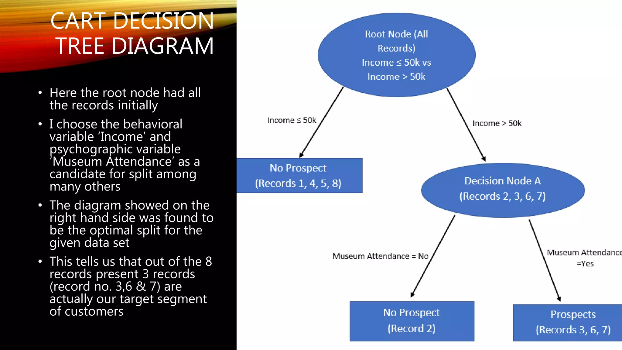
• Here the root node had all
the records initially
• I choose the behavioral
variable ‘Income’ and
psychographic variable
‘Museum Attendance’ as a
candidate for split among
many others
• The diagram showed on the
right hand side was found to
be the optimal split for the
given data set
• This tells us that out of the 8
records present 3 records
(record no. 3,6 & 7) are
actually our target segment
of customers
KANGAROO SEGMENTATION – BAYESIAN MAP
CLASSIFICATION
• In order to find out similar customer
profile, like our loyal customers, among
non-users I use an algorithm called
‘Bayesian Maximum A Priori (MAP)
Classification’
• Here we find a ‘MAP estimate’ of a
customer using our service given some pre
defined criterion
• Using this I could identify two records in
my data set where the ‘MAP estimate’ is
maximum
• These two customers are our loyal
customers
• Any non-user having same demographic
and psychographic profile as these two
customers has the highest potential to
become our customer
Customer
Museum
Attendance
Travel to
India
ExoHind
Prospect
1 Yes No No
2 No Yes No
4 No No No
5 No Yes No
8 No No No
10 No No No
3 Yes Yes Yes 50+, 80k
6 Yes No Yes
7 Yes Yes Yes 50+,65k
9 No Yes Yes
For
Table 1
(when the customer has travelled to India & goes to
museum)
P(Prospect = true) = P(T ꓵ M|EP). P(EP) = 0.5x0.4 = 0.2
P(Prospect = false) = P(T ꓵ M|E̅P̅). P(E̅P̅) = 0x0.6 = 0
VARIOUS ELASTICITY
CALCULATION
Price Promo Online ad TV ad Sales
40 10.5 6.5 6 300
30 10.5 6.5 6 380
30 8 11 7 460
40 11 7 10 540
30 13.5 8 6.5 620
30 14 5 13 700
30 12 10 13 780
40 15 7 19 860
40 15 15 15 940
• The Sales Response function is given by –
Q = K. 𝑃 𝑎. 𝑃𝑟 𝑏. 𝑂𝐴 𝑐. 𝑇𝐴 𝑑 ,
where Q = Sales response function,
K= constant,
P= Price,
Pr = Promotion,
OA= Online advertisement
and TA= Television advertisement
• In order to design the test market to find out the
elasticity values, we use the ‘Before-After’
experimental design methodology
• We get sales data from this test market experiment
• We take logarithms and then run a Regression
Analysis to obtain the values of the various elasticity
co-efficient
• These elasticity values will help me in – calculating
Sales response calculations, pricing strategy and
advertisement budget calculation
Elasticity co-efficient
Price (a) -0.734
Promo (b) 0.727
Online ad (c) 0.361
TV ad (d) 0.570
BRAND AWARENESS AND ADVERTISEMENT – EMPIRICAL
HEM
• Since ExoHind is a start-up so we need a lot of Brand Awareness campaign
• Semiotics principles will be used to design advertisement
• Advertisements and their copies will be inserted in various media
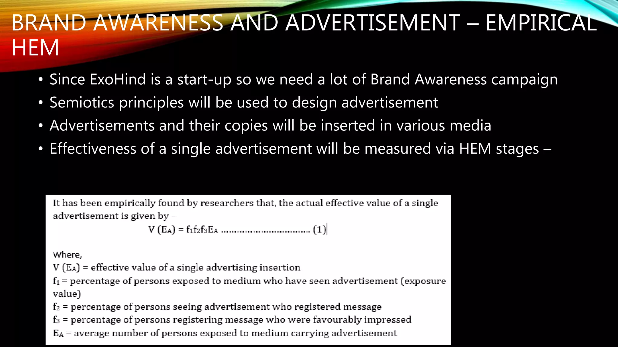
• Effectiveness of a single advertisement will be measured via HEM stages –
MODEL FOR MEASURING BRAND AWARENESS
• I will use Blattberg and Jeuland,1981 model for measuring the effectiveness of a Brand
Awareness campaign
• This model uses ‘Bernoulli advertising exposure process’ and an ‘exponential forgetting
process’ to model awareness
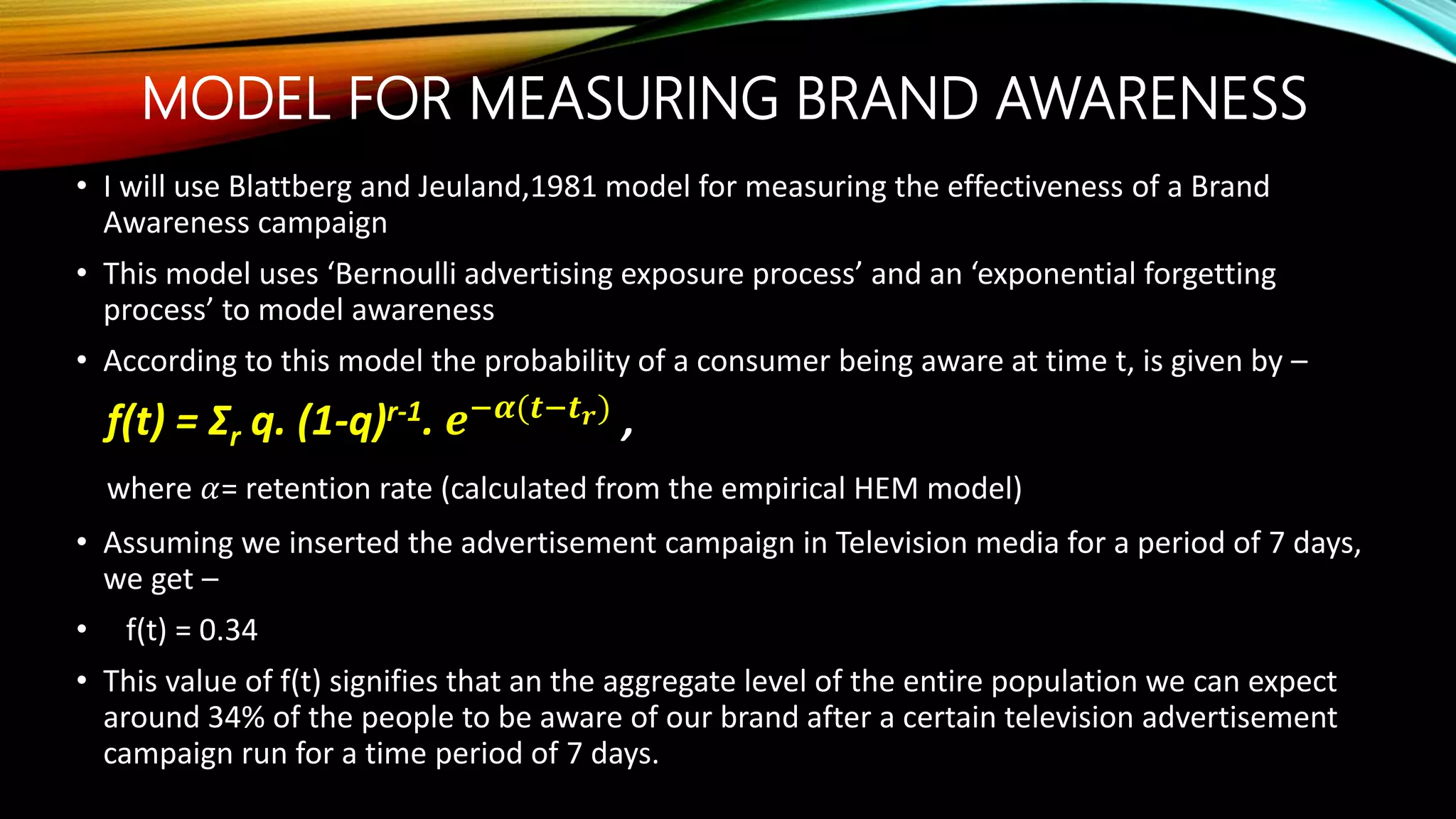
• According to this model the probability of a consumer being aware at time t, is given by –
f(t) = Σr q. (1-q)r-1. 𝒆−𝜶(𝒕−𝒕 𝒓)
,
where 𝛼= retention rate (calculated from the empirical HEM model)
• Assuming we inserted the advertisement campaign in Television media for a period of 7 days,
we get –
• f(t) = 0.34
• This value of f(t) signifies that an the aggregate level of the entire population we can expect
around 34% of the people to be aware of our brand after a certain television advertisement
campaign run for a time period of 7 days.
ADVERTISEMENT BUDGET – VIDALE & WOLFE
MODEL
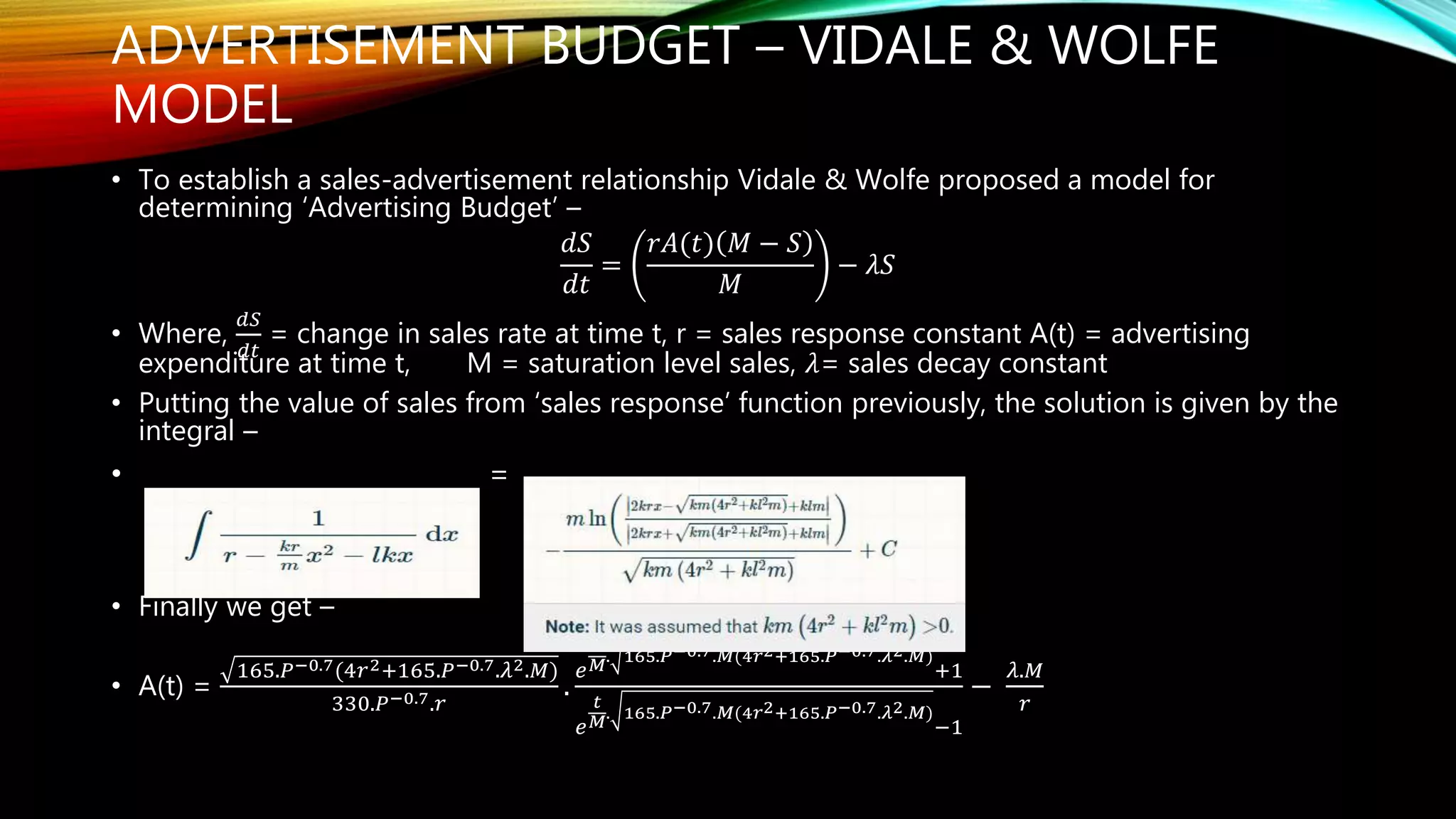
• To establish a sales-advertisement relationship Vidale & Wolfe proposed a model for
determining ‘Advertising Budget’ –
𝑑𝑆
𝑑𝑡
=
𝑟𝐴(𝑡) 𝑀 − 𝑆
𝑀
− 𝜆𝑆
• Where,
𝑑𝑆
𝑑𝑡
= change in sales rate at time t, r = sales response constant A(t) = advertising
expenditure at time t, M = saturation level sales, 𝜆= sales decay constant
• Putting the value of sales from ‘sales response’ function previously, the solution is given by the
integral –
• =
• Finally we get –
• A(t) =
165.𝑃−0.7(4𝑟2+165.𝑃−0.7.𝜆2.𝑀)
330.𝑃−0.7.𝑟
.
𝑒
𝑡
𝑀
. 165.𝑃−0.7.𝑀(4𝑟2+165.𝑃−0.7.𝜆2.𝑀)
+1
𝑒
𝑡
𝑀
. 165.𝑃−0.7.𝑀(4𝑟2+165.𝑃−0.7.𝜆2.𝑀)
−1
−
𝜆.𝑀
𝑟
PRICING STRATEGY – DOCKNER & JORGENSEN
MODEL
• We will set our price using competitive pricing
– using Dockner & Jorgensen model (1988)
• This model assumes an open-loop Nash
equilibrium concept where each firm is
assumed to optimize its price time path, given
knowledge of what all other firms are doing
• Optimal price according to this is given by –
Dockner-
Jorgensen Model
This
Year
Next
Year
Next Year
with EH
Differe
nce
Sales
Lost (λ)
Elastici
ty
MMT Market
Share = 88320
11408
1 102599 11482 0.48 0.72
Yatra Market
Share = 44160 57041 51300 5741 0.24 0.76
ExoHind Market
Share = 0 0 23921 0 0.73
Others = 51520 66547 59849 6698 0.28 0.77
Optimal price
= $ 903
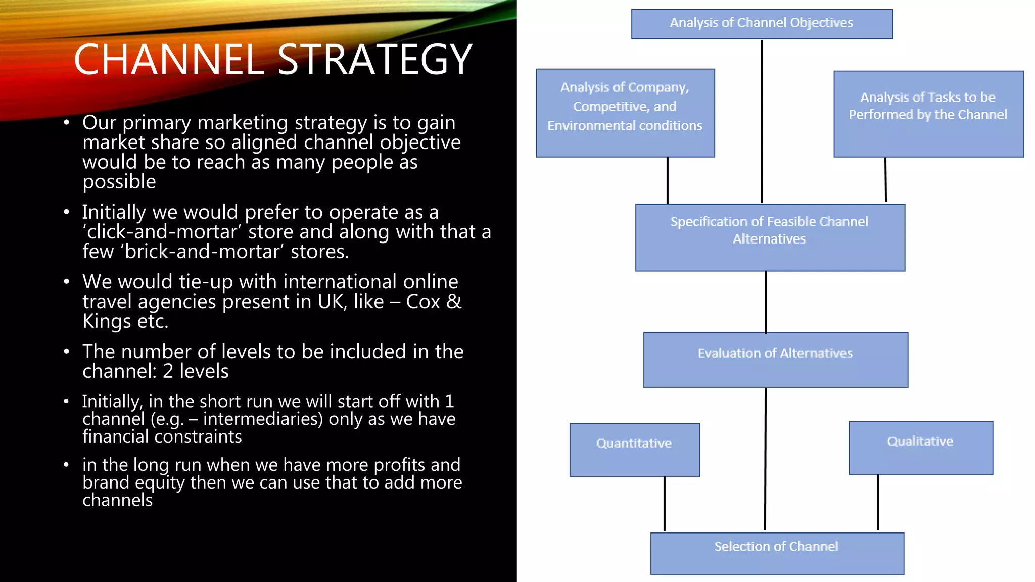
CHANNEL STRATEGY
• Our primary marketing strategy is to gain
market share so aligned channel objective
would be to reach as many people as
possible
• Initially we would prefer to operate as a
‘click-and-mortar’ store and along with that a
few ‘brick-and-mortar’ stores.
• We would tie-up with international online
travel agencies present in UK, like – Cox &
Kings etc.
• The number of levels to be included in the
channel: 2 levels
• Initially, in the short run we will start off with 1
channel (e.g. – intermediaries) only as we have
financial constraints
• in the long run when we have more profits and
brand equity then we can use that to add more
channels

Marketing strategy exo hind

  • 1.
    MARKETING STRATEGY EXOHIND -HIGHLIGHTS Presented by Soumyadeep Chowdhury
  • 2.
    EXOHIND GROWTH PLAN– EXTENDED BDM • ‘ExoHind’ is a start-up company that is funded partly by seed capital of the founding members and partly by taking loan and going to start a business in the Lifestyle travel category • Since this is a start-up so I don’t have any sales data for it • In order to forecast our sales I used Brand level extension of Bass Diffusion Model – • Then we use the Funds Balance Equation to identify the expected growth rate Year 1 Year 2 Year 3 Revenue 21576742 22929742 24282742 Growth Rate 0 6.27 5.90 Expenses 5000000 5000000 5000000 Profit 16576742 17929742 19282742 RONA 2.81 3.04 3.27 debt/equity 0.50 1.50 2.00 retained earning ratio r 0.77 0.78 0.79 g(s) 3.20 5.82 7.79
  • 3.
    BRAND ATTRIBUTES &IMPORTANCE - FISHBEIN • We use the reverse fishbein model to find out the relative importance of the three attributes that are relevant for us • We found the rough estimates of market shares of the various competitors for previous year • For this year we use Bass Diffusion model to forecast category level sales and calculate market share • From that market share we find out attitude and then run a Regression analysis on Brand Attitudes and beliefs to find out the ‘Importance’ ratings Attributes MakemyT rip Yatra ExoHind Others Importan ce Arts & Cultural value 7 6 9 8 b1 = 5 Website quality 7 6 8 7 b2 = 14 Travel experience in India 9 8 7 8 b3 = 81 Attitude A1 = 10.58 A2 = 5.29 A3 = 2.47 A4 = 6.17 100 Market Share 0.432 0.216 0.101 0.252 1.000
  • 4.
    CLASSIFICATION AND REGRESSIONTREE SEGMENTATION • Here I have taken a representative data set of customers, based on various demographic and psychographic attributes • Then I use CART algorithm on that data set • This algorithm basically divides the records in the data set into various decision nodes based on the criterion mentioned in the candidate split • Each split gives us a set of nodes • We measure ‘Φ’ – the goodness of split for each candidate splits • Φ(s|t) = 2 PLPR 𝑗 # 𝐶𝑙𝑎𝑠𝑠𝑒𝑠 | 𝑃 𝑗 𝑡 𝐿 − 𝑃(𝑗|𝑡 𝑅)| • The split with highest ‘Φ’ value gives us the desired segment Custom er Income Age Internet Museum Attendance Travel to India ExoHind Prospect 1 30k 20-30 No Yes No No 2 50k 30-40 Yes No Yes No 3 80k 50+ Yes Yes Yes Yes 4 30k 20-30 Yes No No No 5 45k 30-40 Yes No Yes No 6 55k 30-40 Yes Yes No Yes 7 65k 50+ Yes Yes Yes Yes 8 40k 20-30 Yes No No No No Left child node, t(L) Right child node, t(R ) 1 Internet = no Internet = yes 2 Travel to India = no Travel to India = yes 3 Museum attendance = no Museum attendance = yes 4 Age <= 30 Age>30 5 Age <= 40 Age>40 6 Age <= 50 Age>50 7 Income <= 30k Income>30k 8 Income <= 50k Income>50k 9 Income <= 75k Income> 75k
  • 5.
    CART DECISION TREE DIAGRAM •Here the root node had all the records initially • I choose the behavioral variable ‘Income’ and psychographic variable ‘Museum Attendance’ as a candidate for split among many others • The diagram showed on the right hand side was found to be the optimal split for the given data set • This tells us that out of the 8 records present 3 records (record no. 3,6 & 7) are actually our target segment of customers
  • 6.
    KANGAROO SEGMENTATION –BAYESIAN MAP CLASSIFICATION • In order to find out similar customer profile, like our loyal customers, among non-users I use an algorithm called ‘Bayesian Maximum A Priori (MAP) Classification’ • Here we find a ‘MAP estimate’ of a customer using our service given some pre defined criterion • Using this I could identify two records in my data set where the ‘MAP estimate’ is maximum • These two customers are our loyal customers • Any non-user having same demographic and psychographic profile as these two customers has the highest potential to become our customer Customer Museum Attendance Travel to India ExoHind Prospect 1 Yes No No 2 No Yes No 4 No No No 5 No Yes No 8 No No No 10 No No No 3 Yes Yes Yes 50+, 80k 6 Yes No Yes 7 Yes Yes Yes 50+,65k 9 No Yes Yes For Table 1 (when the customer has travelled to India & goes to museum) P(Prospect = true) = P(T ꓵ M|EP). P(EP) = 0.5x0.4 = 0.2 P(Prospect = false) = P(T ꓵ M|E̅P̅). P(E̅P̅) = 0x0.6 = 0
  • 7.
    VARIOUS ELASTICITY CALCULATION Price PromoOnline ad TV ad Sales 40 10.5 6.5 6 300 30 10.5 6.5 6 380 30 8 11 7 460 40 11 7 10 540 30 13.5 8 6.5 620 30 14 5 13 700 30 12 10 13 780 40 15 7 19 860 40 15 15 15 940 • The Sales Response function is given by – Q = K. 𝑃 𝑎. 𝑃𝑟 𝑏. 𝑂𝐴 𝑐. 𝑇𝐴 𝑑 , where Q = Sales response function, K= constant, P= Price, Pr = Promotion, OA= Online advertisement and TA= Television advertisement • In order to design the test market to find out the elasticity values, we use the ‘Before-After’ experimental design methodology • We get sales data from this test market experiment • We take logarithms and then run a Regression Analysis to obtain the values of the various elasticity co-efficient • These elasticity values will help me in – calculating Sales response calculations, pricing strategy and advertisement budget calculation Elasticity co-efficient Price (a) -0.734 Promo (b) 0.727 Online ad (c) 0.361 TV ad (d) 0.570
  • 8.
    BRAND AWARENESS ANDADVERTISEMENT – EMPIRICAL HEM • Since ExoHind is a start-up so we need a lot of Brand Awareness campaign • Semiotics principles will be used to design advertisement • Advertisements and their copies will be inserted in various media • Effectiveness of a single advertisement will be measured via HEM stages –
  • 9.
    MODEL FOR MEASURINGBRAND AWARENESS • I will use Blattberg and Jeuland,1981 model for measuring the effectiveness of a Brand Awareness campaign • This model uses ‘Bernoulli advertising exposure process’ and an ‘exponential forgetting process’ to model awareness • According to this model the probability of a consumer being aware at time t, is given by – f(t) = Σr q. (1-q)r-1. 𝒆−𝜶(𝒕−𝒕 𝒓) , where 𝛼= retention rate (calculated from the empirical HEM model) • Assuming we inserted the advertisement campaign in Television media for a period of 7 days, we get – • f(t) = 0.34 • This value of f(t) signifies that an the aggregate level of the entire population we can expect around 34% of the people to be aware of our brand after a certain television advertisement campaign run for a time period of 7 days.
  • 10.
    ADVERTISEMENT BUDGET –VIDALE & WOLFE MODEL • To establish a sales-advertisement relationship Vidale & Wolfe proposed a model for determining ‘Advertising Budget’ – 𝑑𝑆 𝑑𝑡 = 𝑟𝐴(𝑡) 𝑀 − 𝑆 𝑀 − 𝜆𝑆 • Where, 𝑑𝑆 𝑑𝑡 = change in sales rate at time t, r = sales response constant A(t) = advertising expenditure at time t, M = saturation level sales, 𝜆= sales decay constant • Putting the value of sales from ‘sales response’ function previously, the solution is given by the integral – • = • Finally we get – • A(t) = 165.𝑃−0.7(4𝑟2+165.𝑃−0.7.𝜆2.𝑀) 330.𝑃−0.7.𝑟 . 𝑒 𝑡 𝑀 . 165.𝑃−0.7.𝑀(4𝑟2+165.𝑃−0.7.𝜆2.𝑀) +1 𝑒 𝑡 𝑀 . 165.𝑃−0.7.𝑀(4𝑟2+165.𝑃−0.7.𝜆2.𝑀) −1 − 𝜆.𝑀 𝑟
  • 11.
    PRICING STRATEGY –DOCKNER & JORGENSEN MODEL • We will set our price using competitive pricing – using Dockner & Jorgensen model (1988) • This model assumes an open-loop Nash equilibrium concept where each firm is assumed to optimize its price time path, given knowledge of what all other firms are doing • Optimal price according to this is given by – Dockner- Jorgensen Model This Year Next Year Next Year with EH Differe nce Sales Lost (λ) Elastici ty MMT Market Share = 88320 11408 1 102599 11482 0.48 0.72 Yatra Market Share = 44160 57041 51300 5741 0.24 0.76 ExoHind Market Share = 0 0 23921 0 0.73 Others = 51520 66547 59849 6698 0.28 0.77 Optimal price = $ 903
  • 12.
    CHANNEL STRATEGY • Ourprimary marketing strategy is to gain market share so aligned channel objective would be to reach as many people as possible • Initially we would prefer to operate as a ‘click-and-mortar’ store and along with that a few ‘brick-and-mortar’ stores. • We would tie-up with international online travel agencies present in UK, like – Cox & Kings etc. • The number of levels to be included in the channel: 2 levels • Initially, in the short run we will start off with 1 channel (e.g. – intermediaries) only as we have financial constraints • in the long run when we have more profits and brand equity then we can use that to add more channels