Download as PDF, PPTX
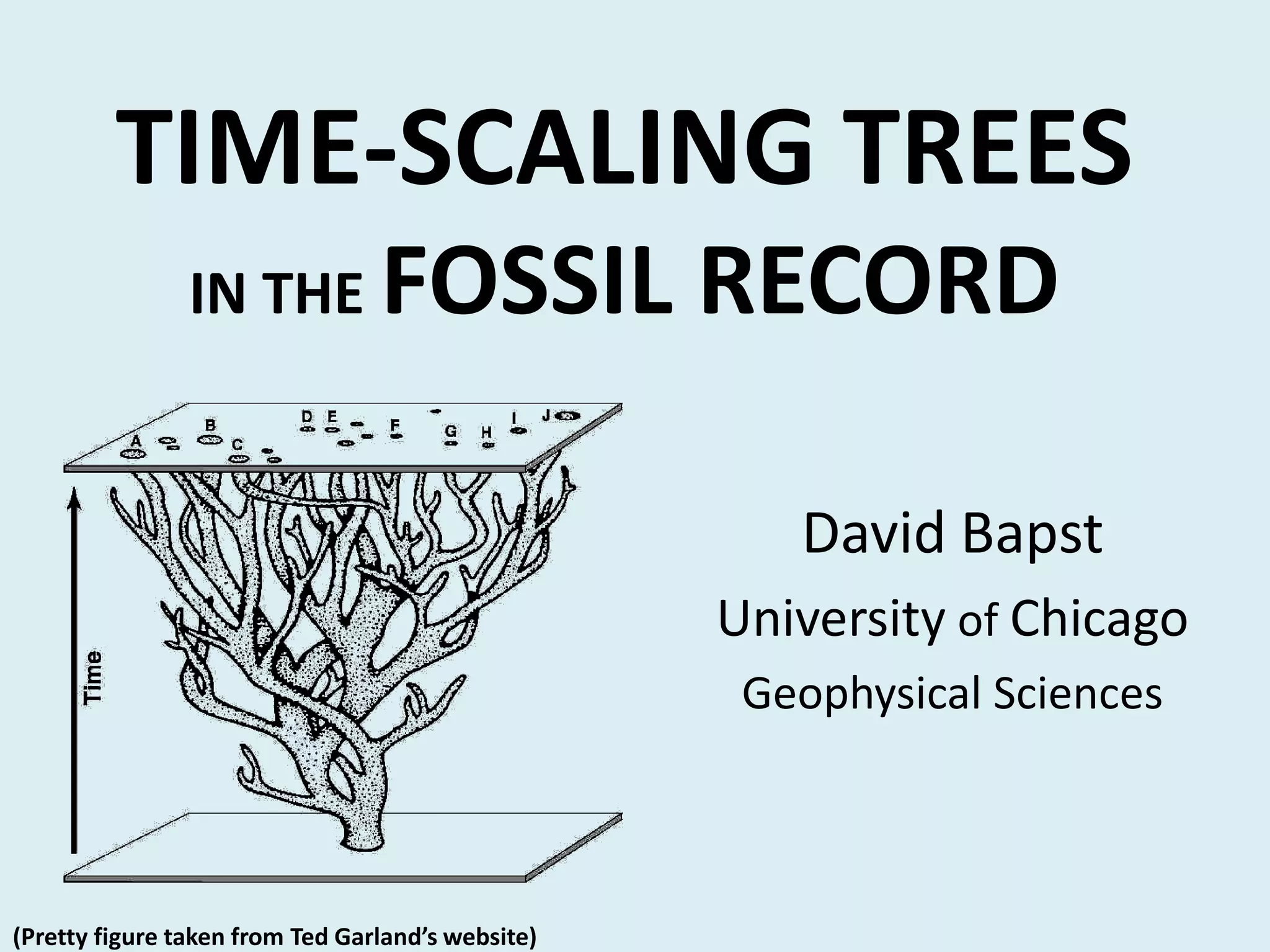
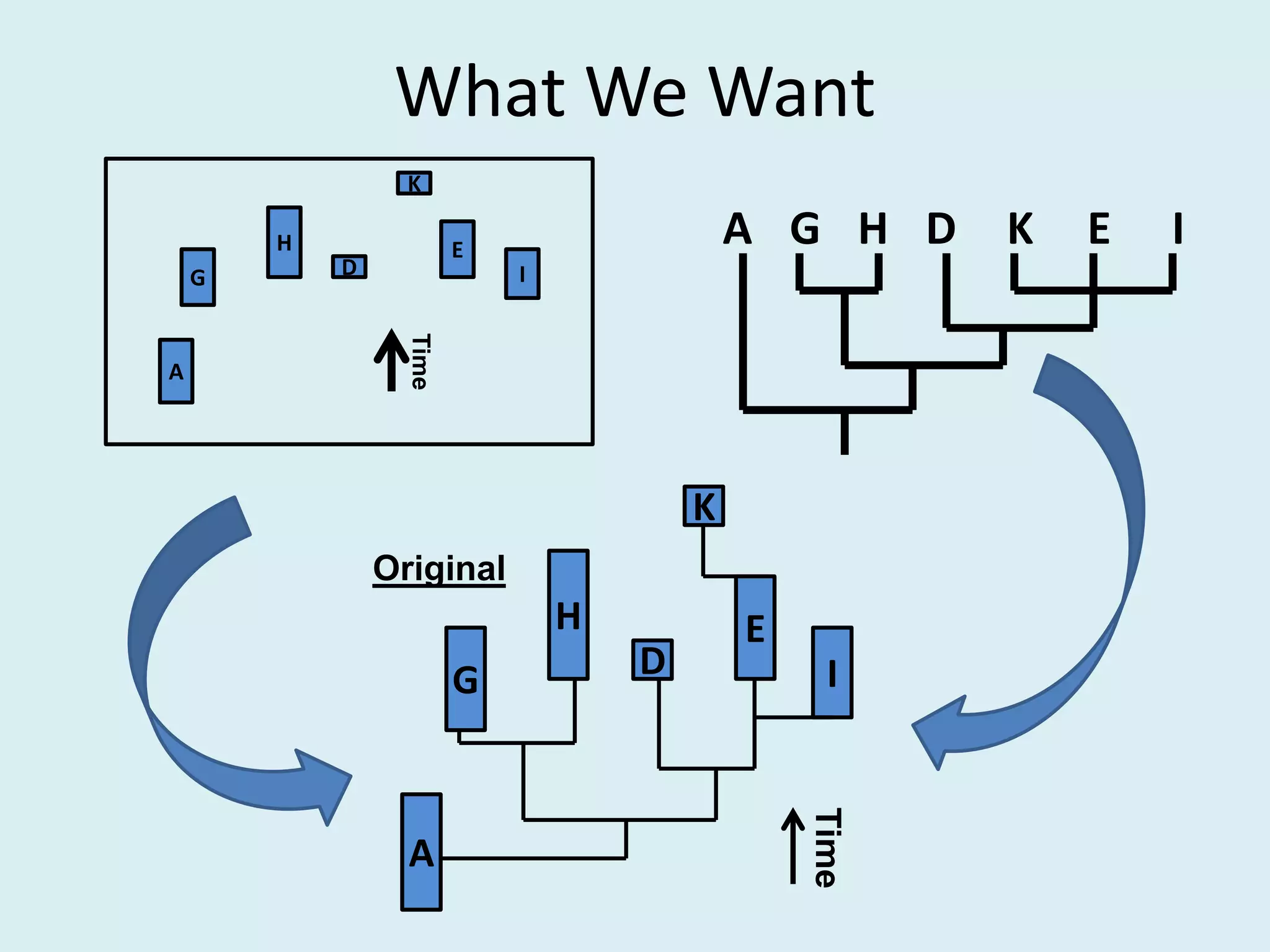
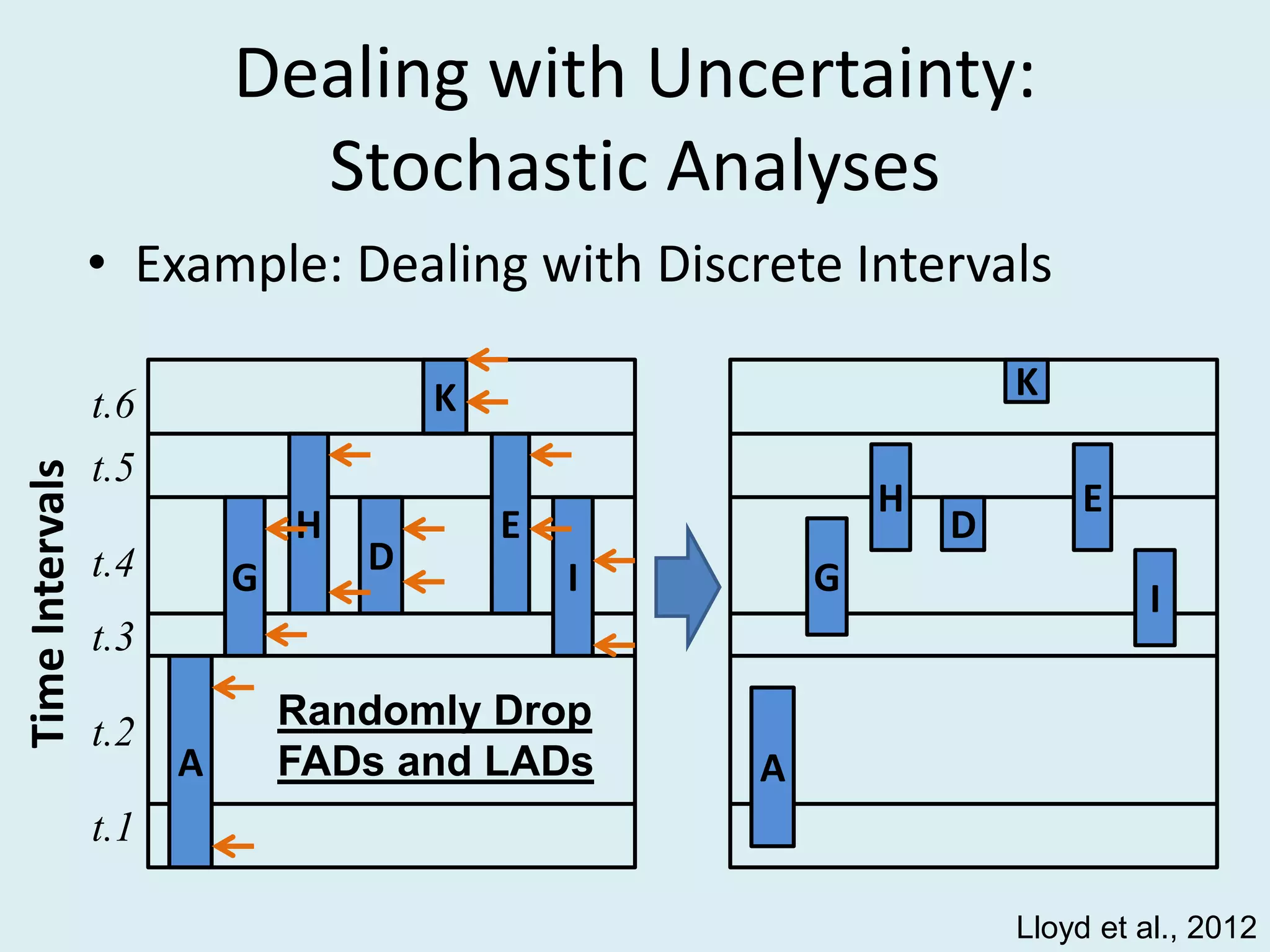
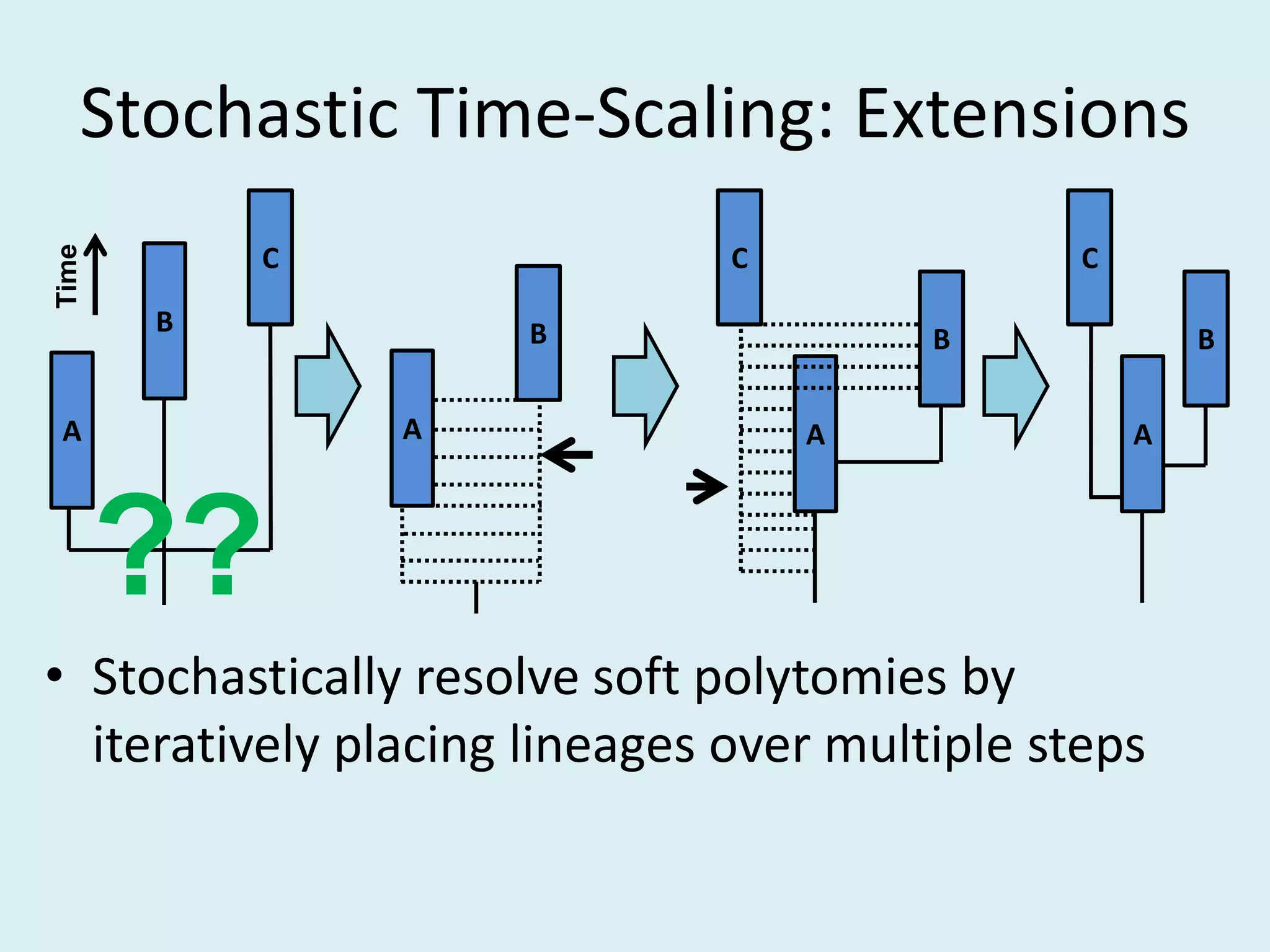
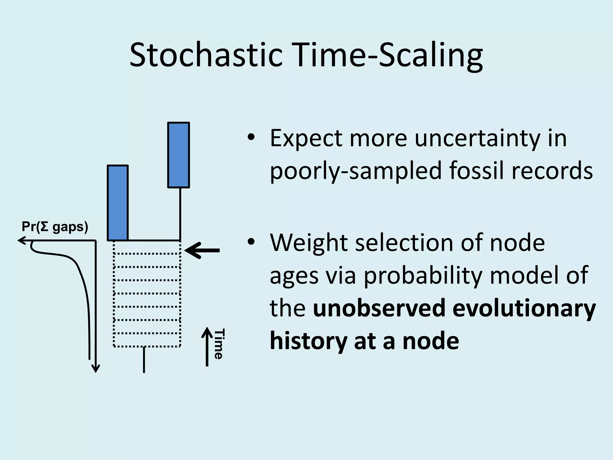
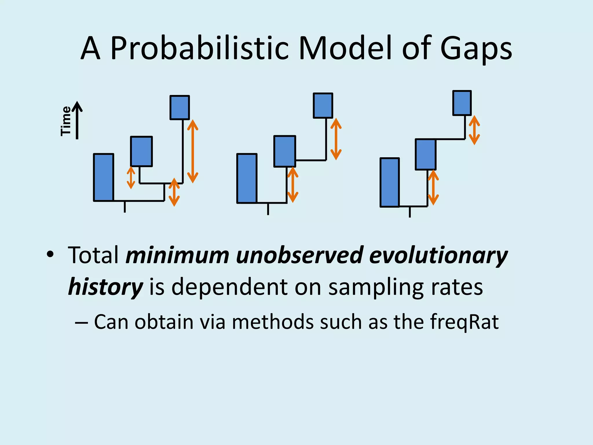
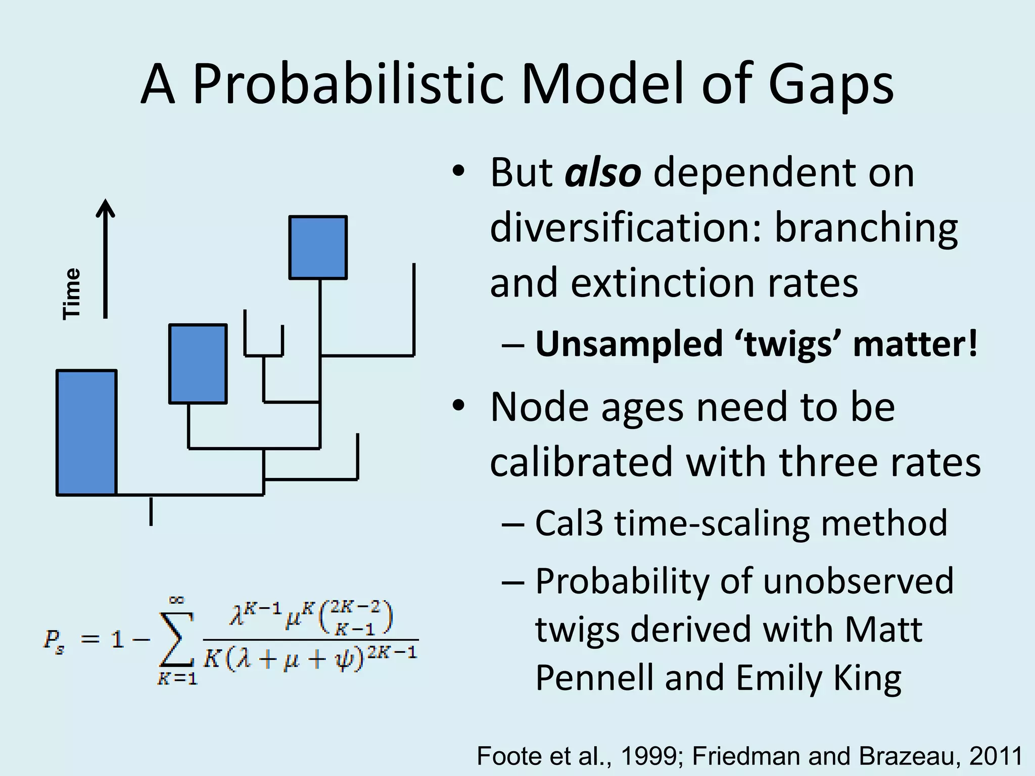
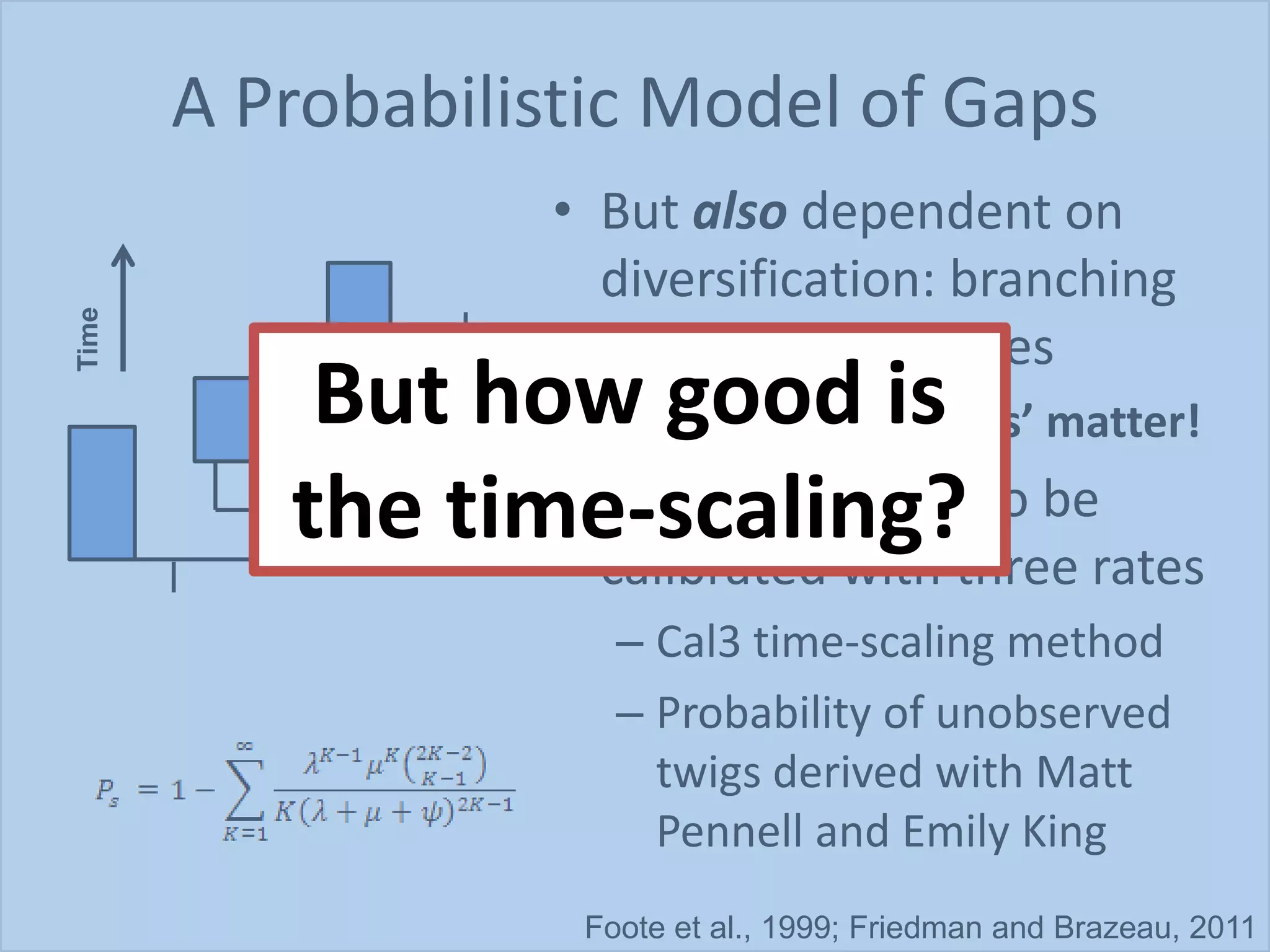
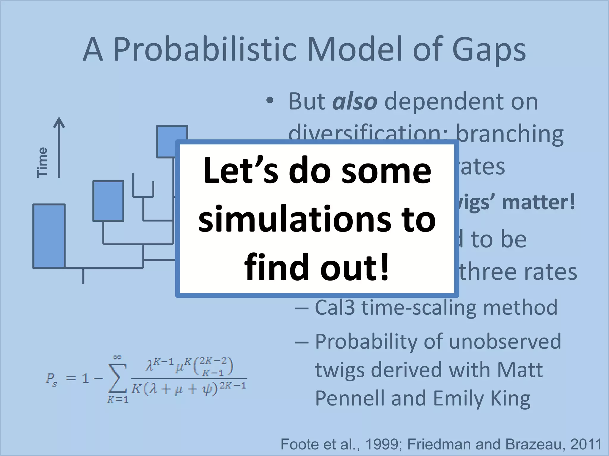
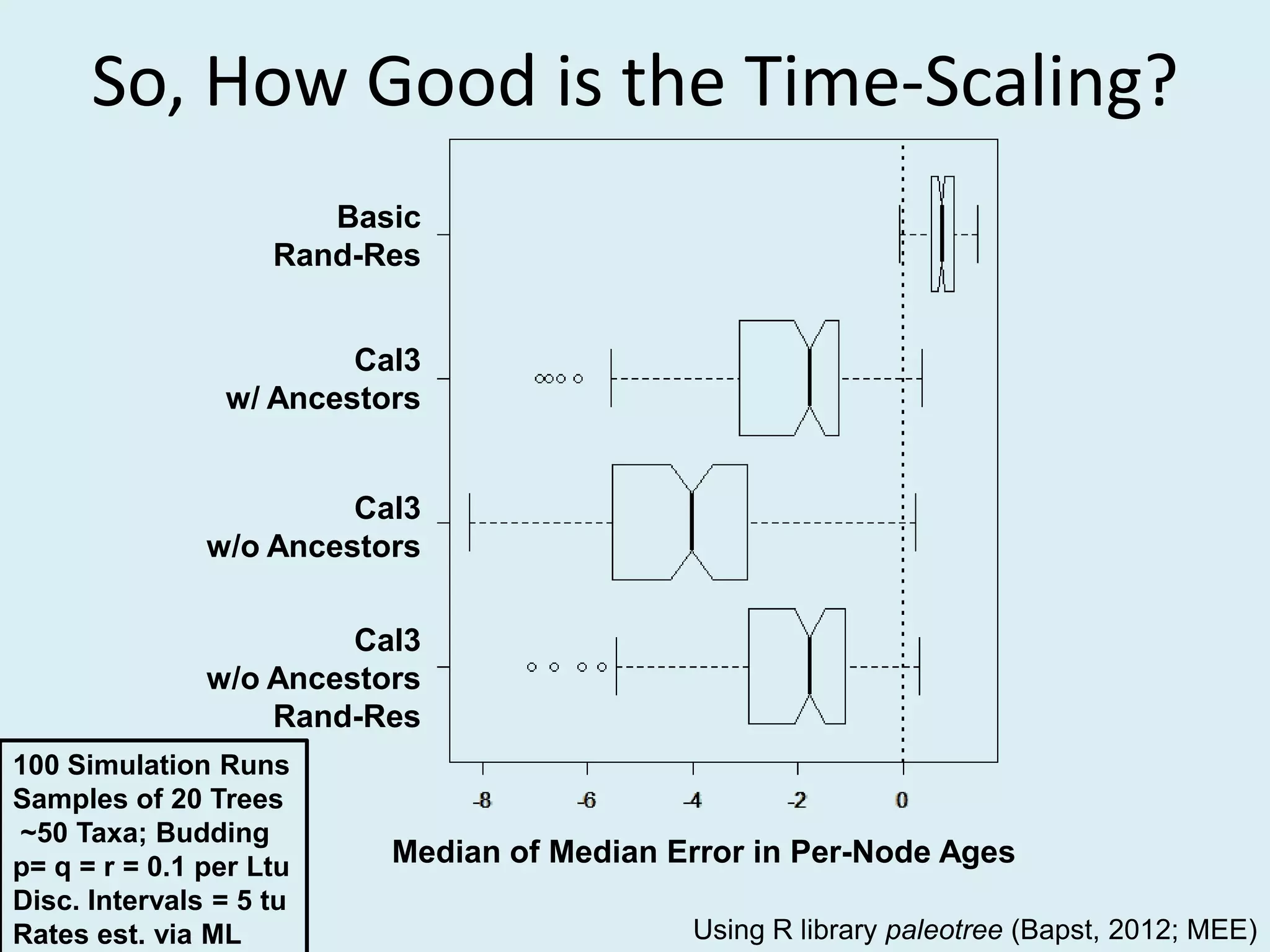
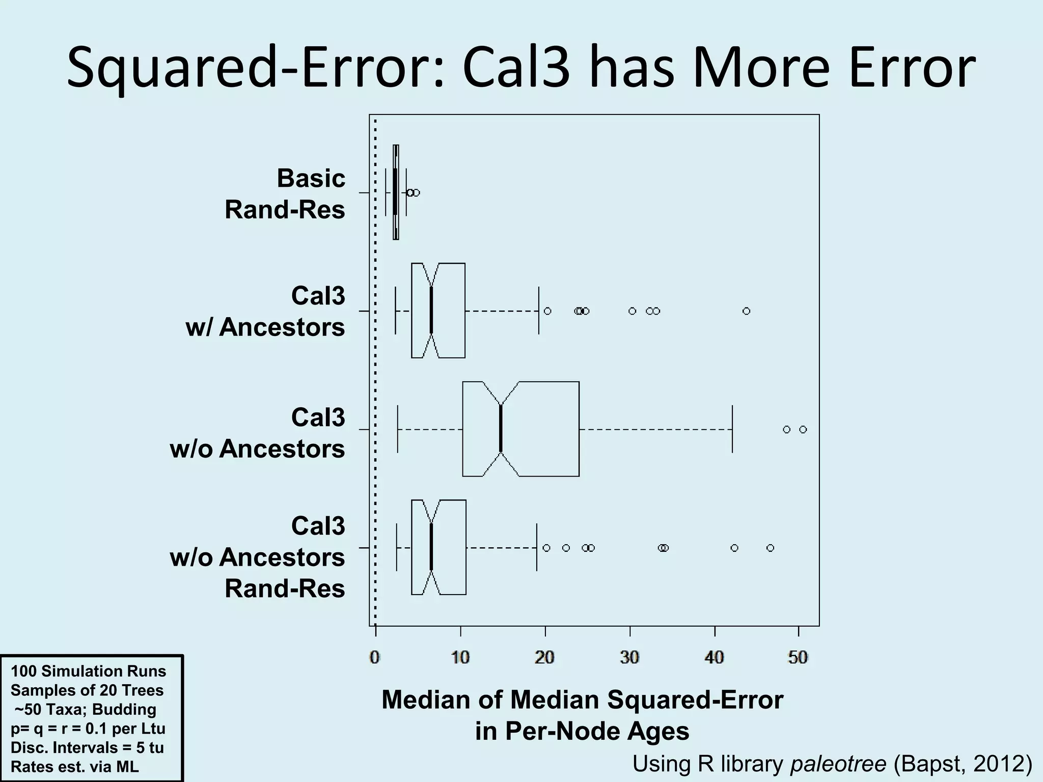
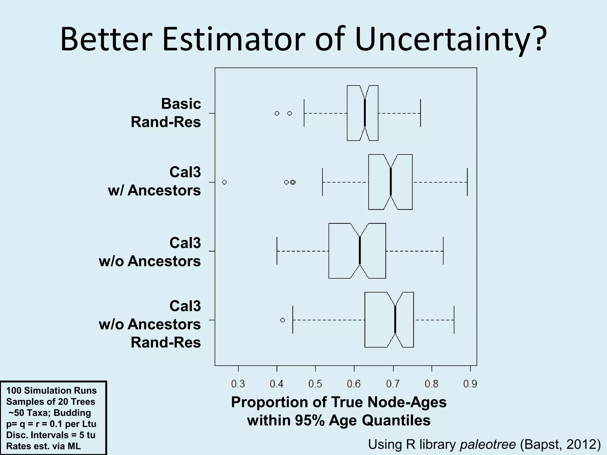
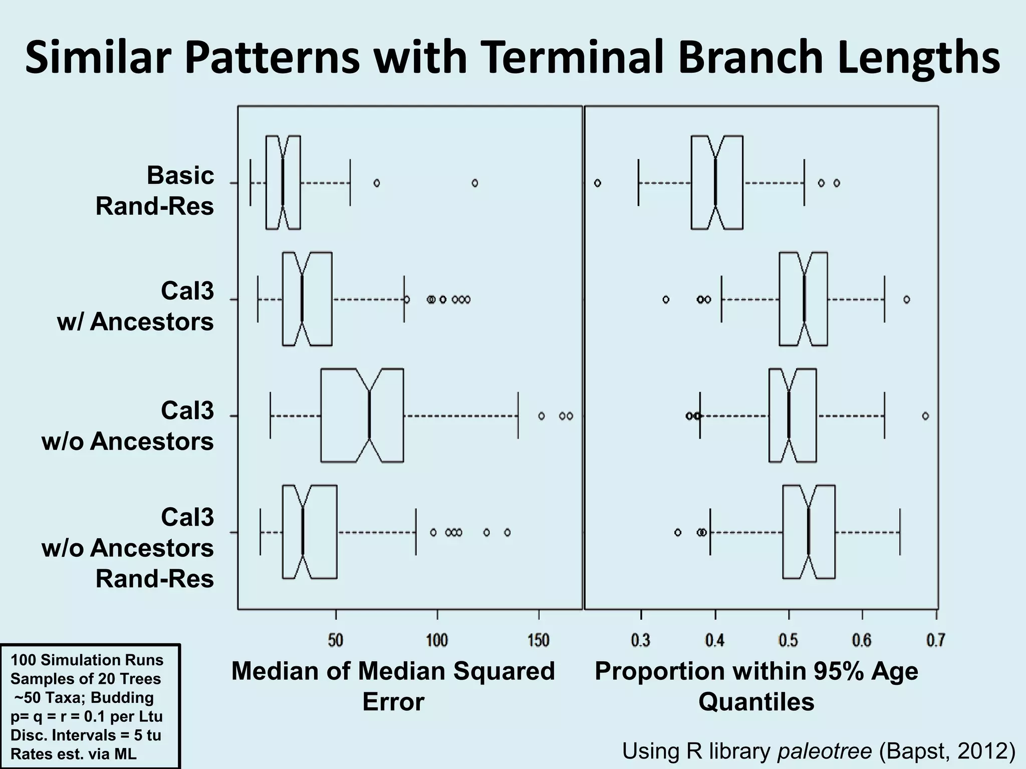
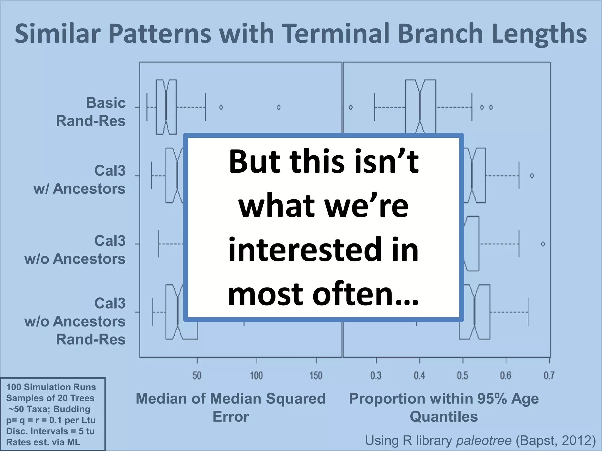
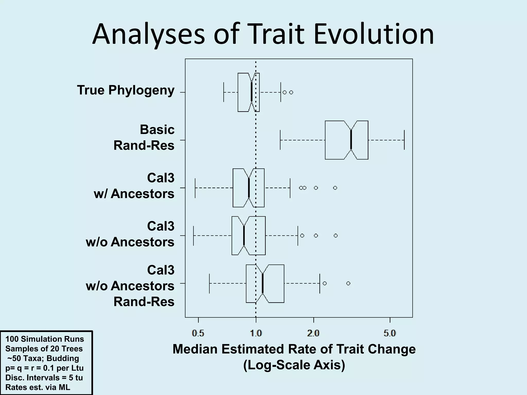
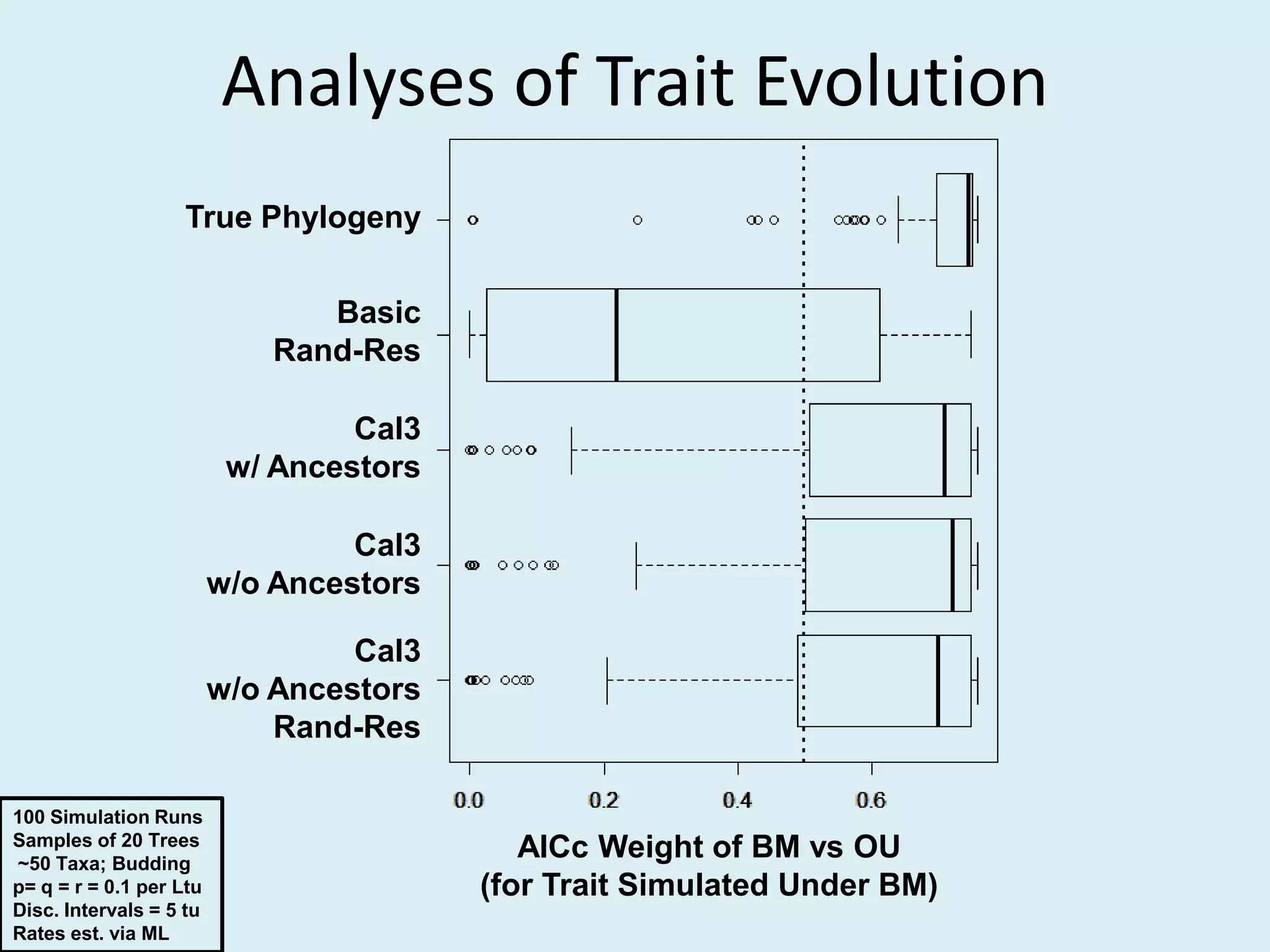
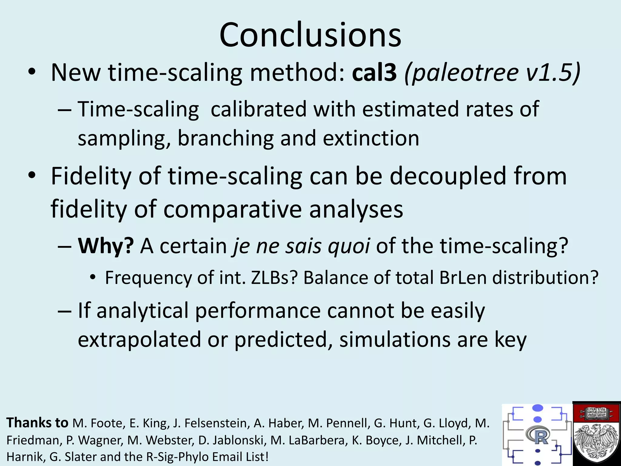


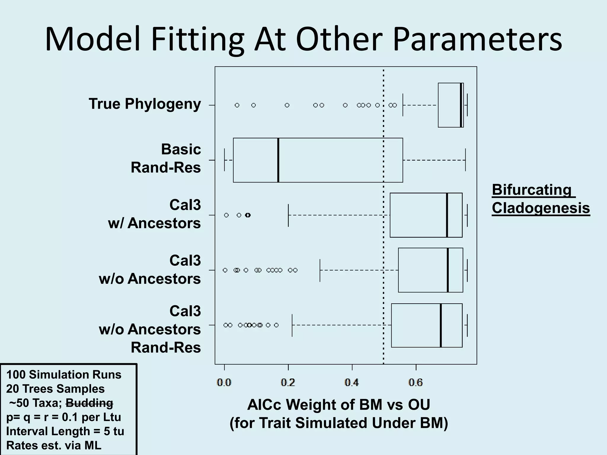
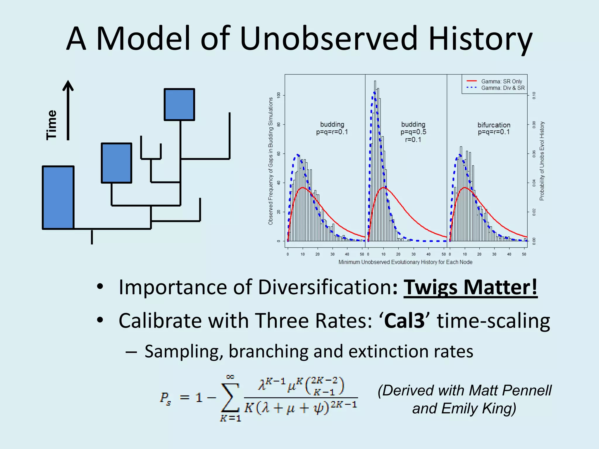


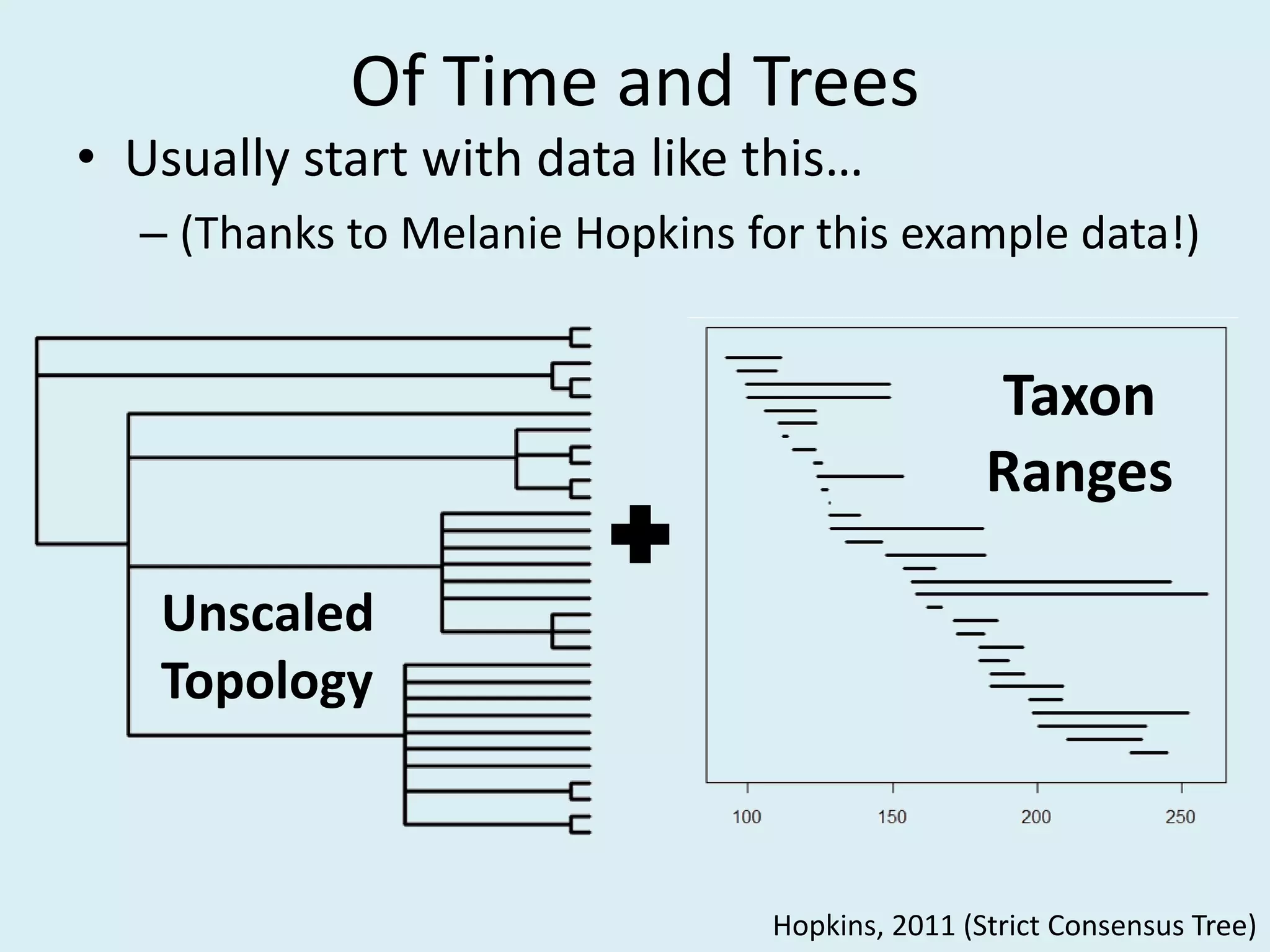
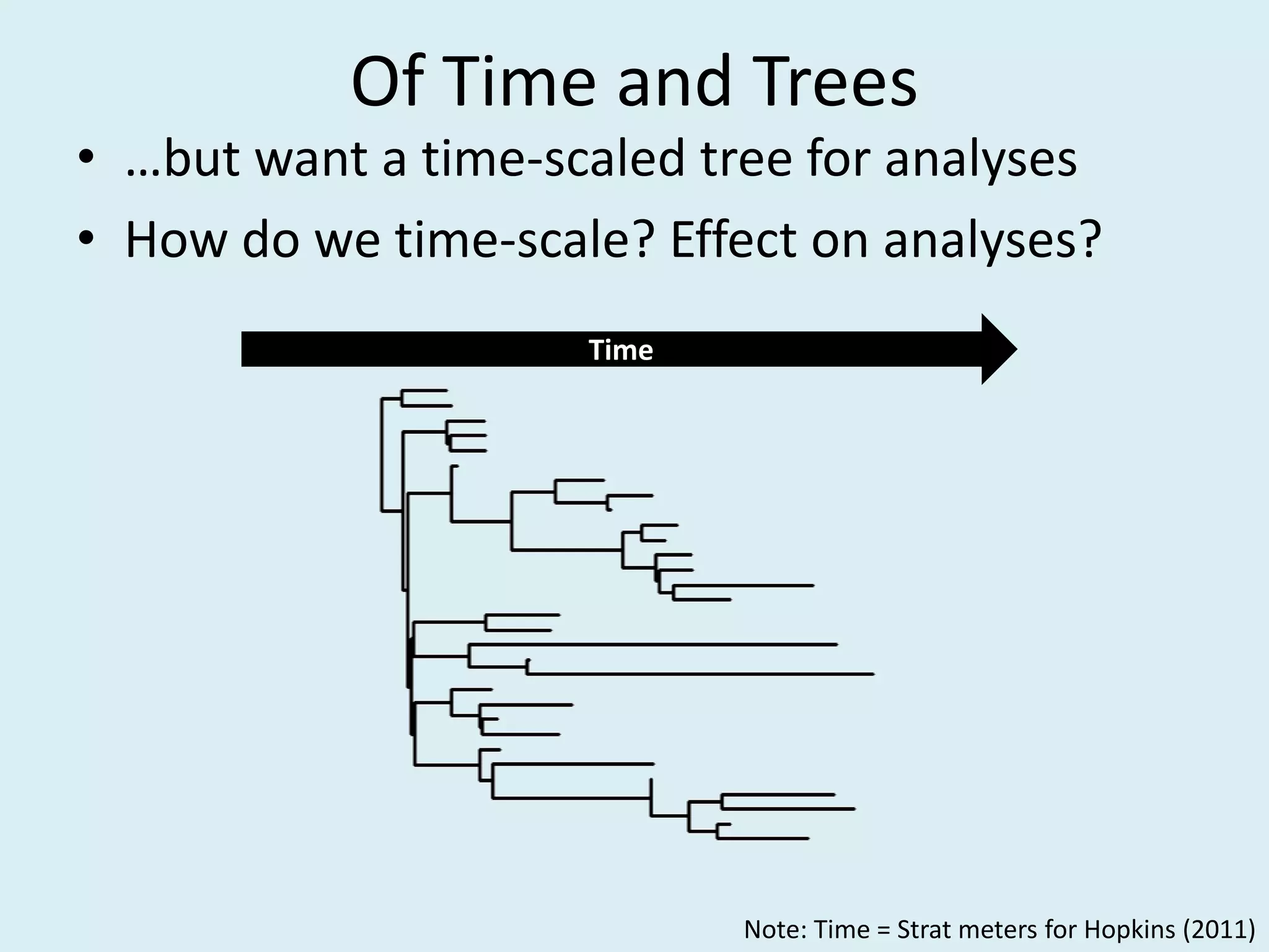
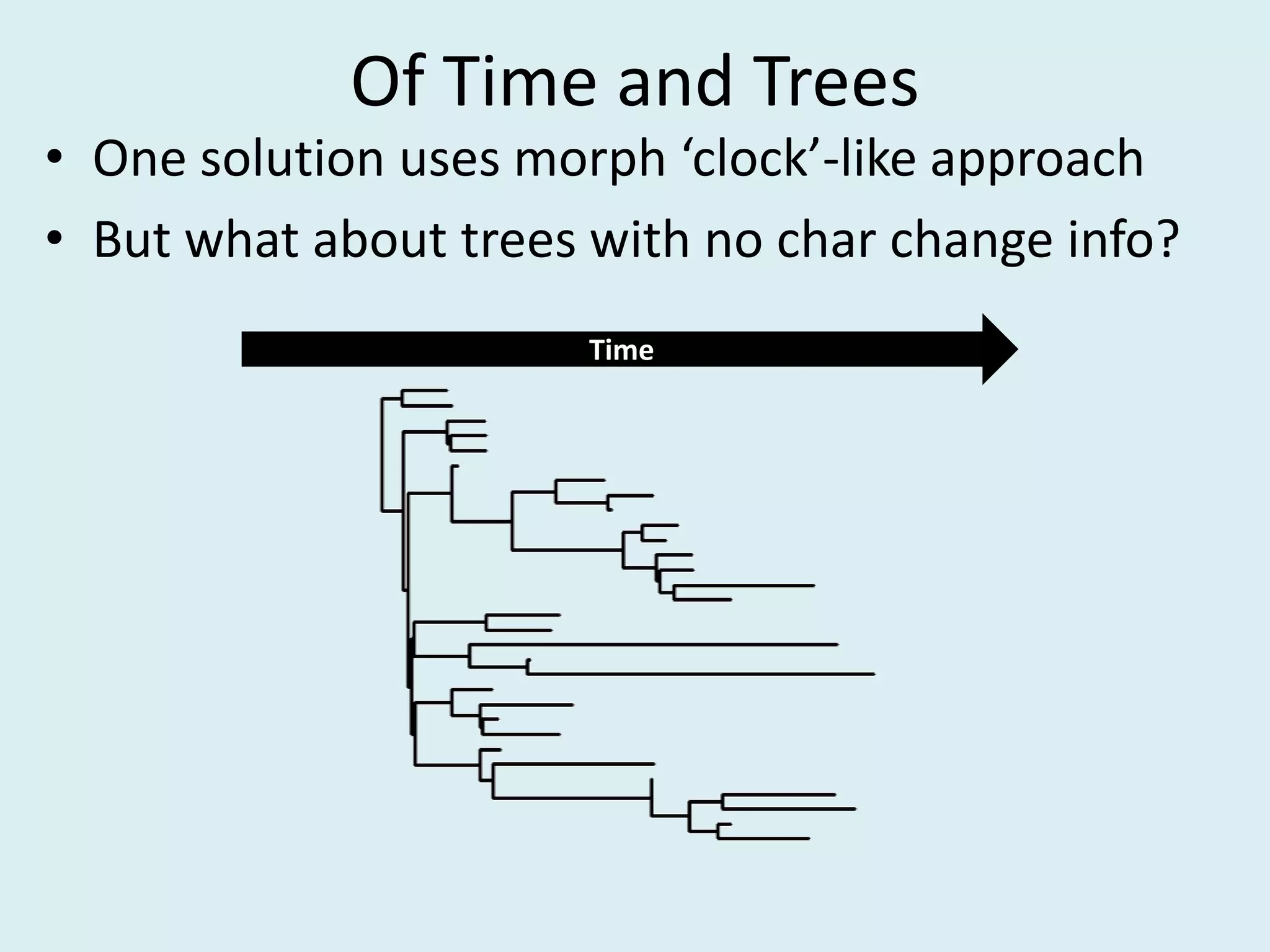
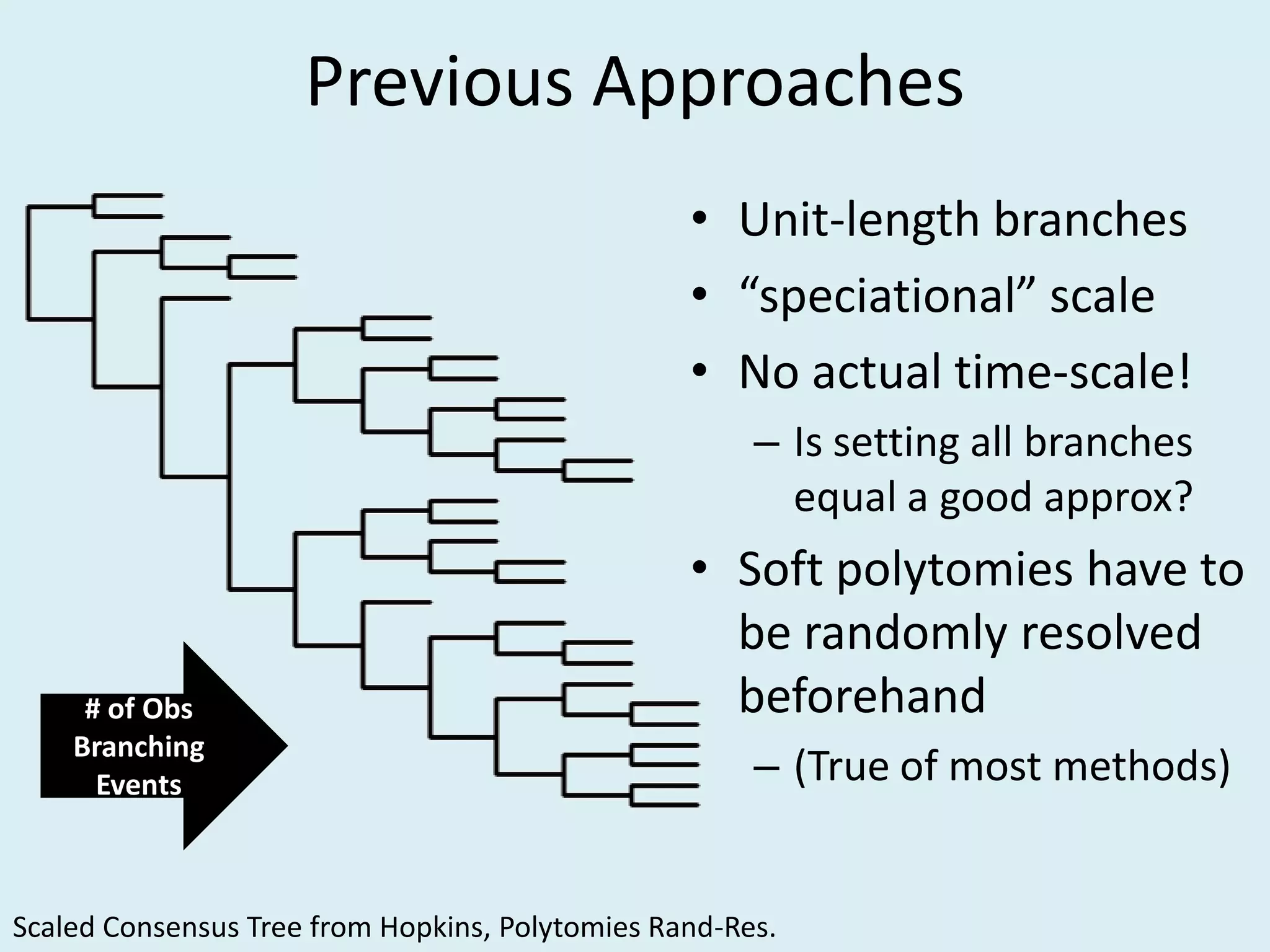
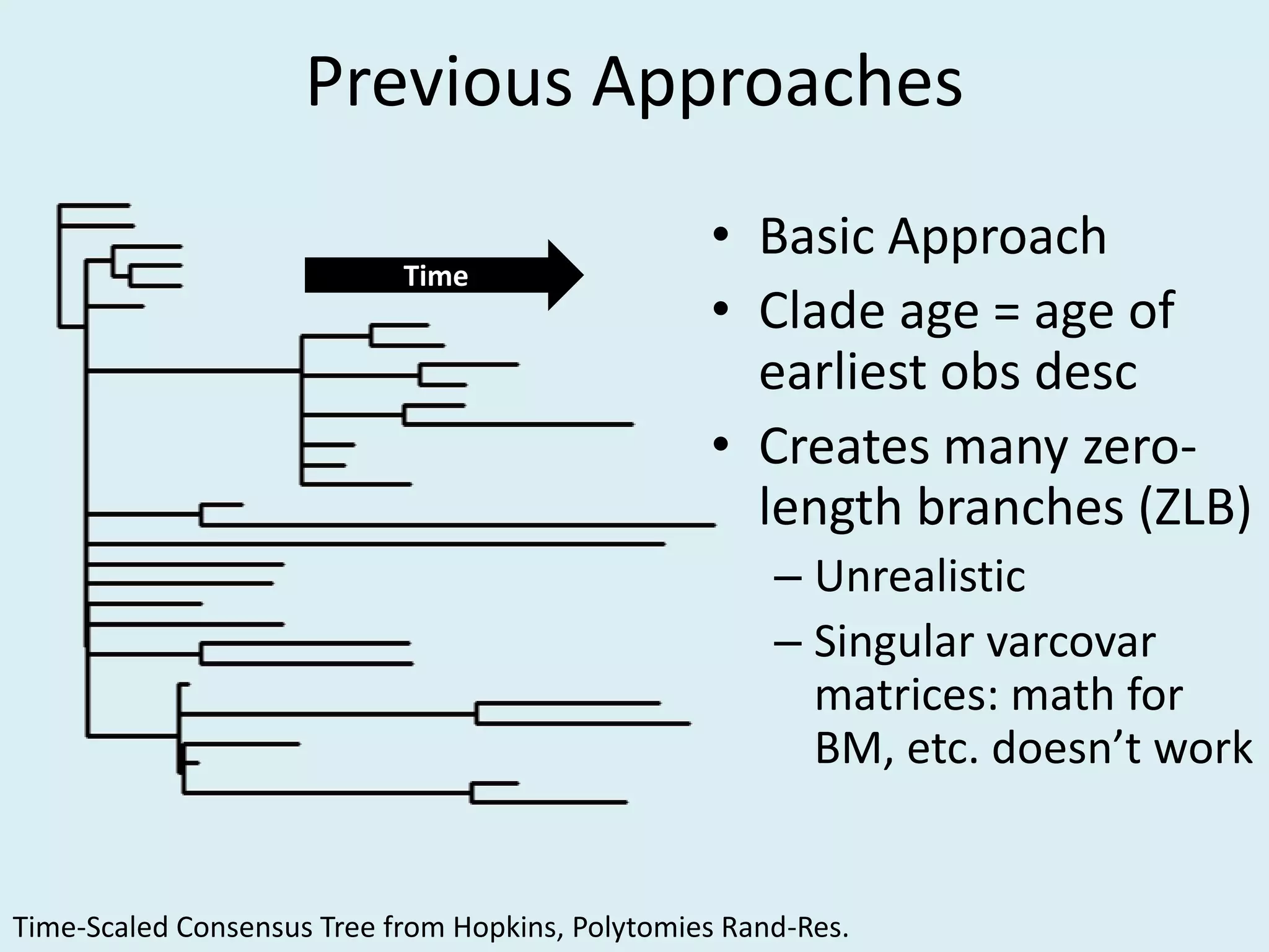
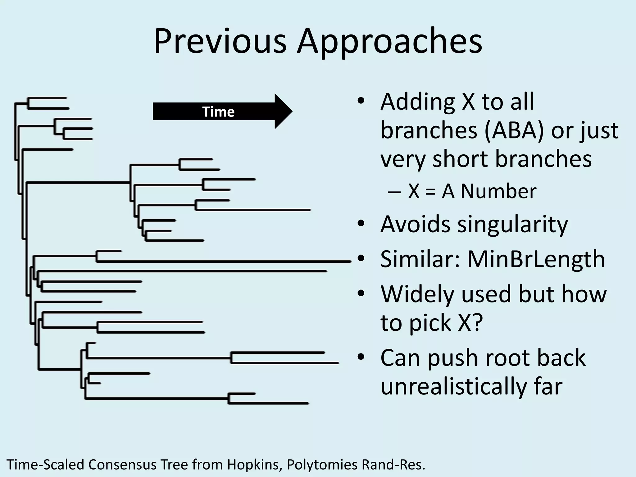
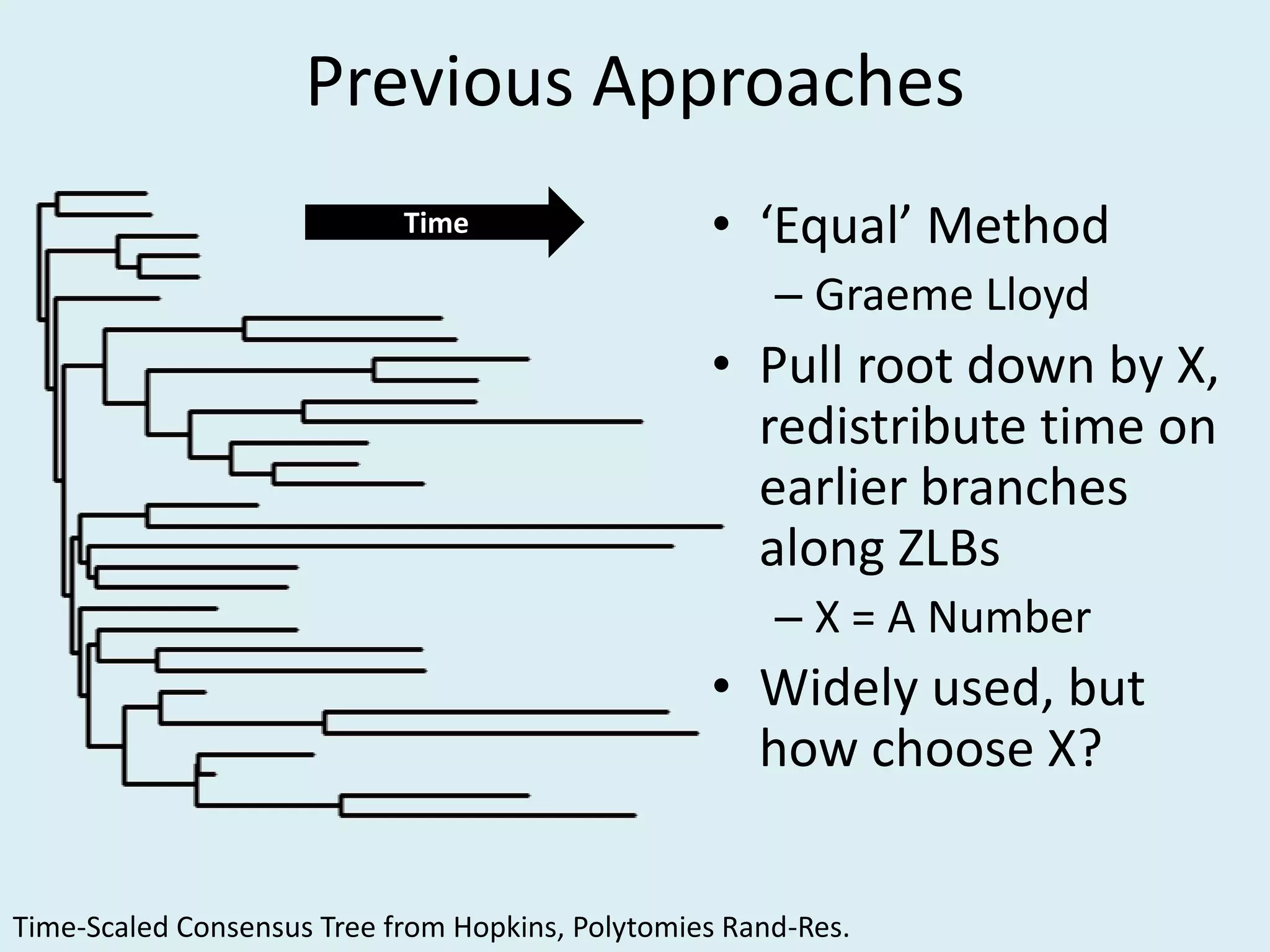
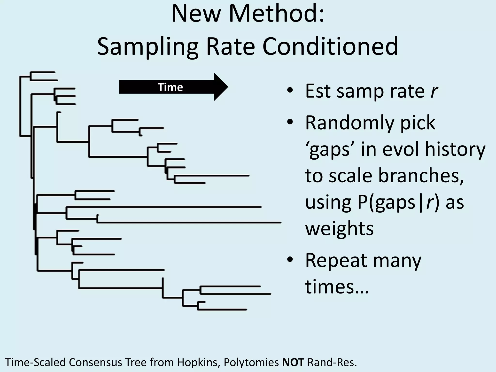
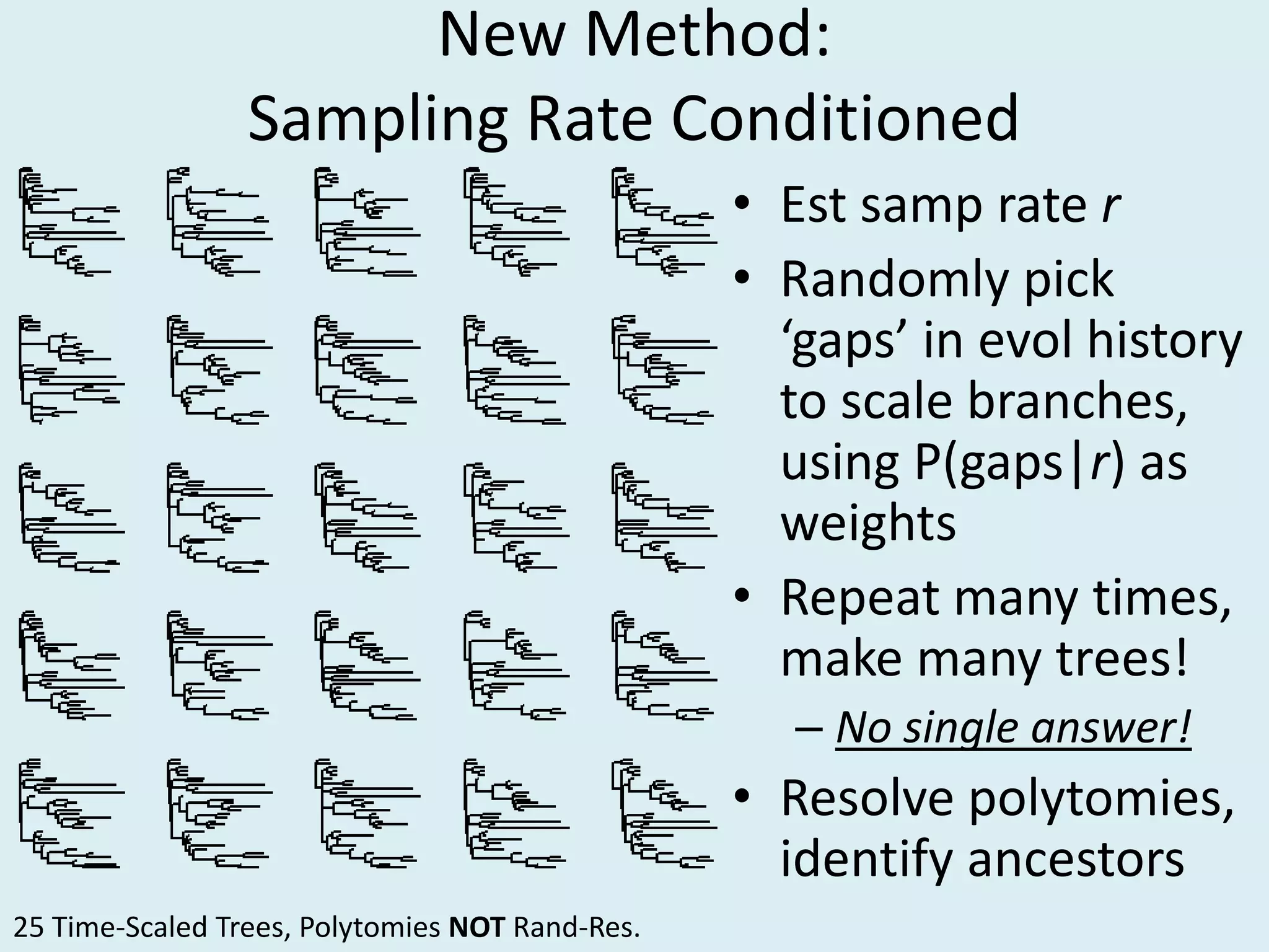

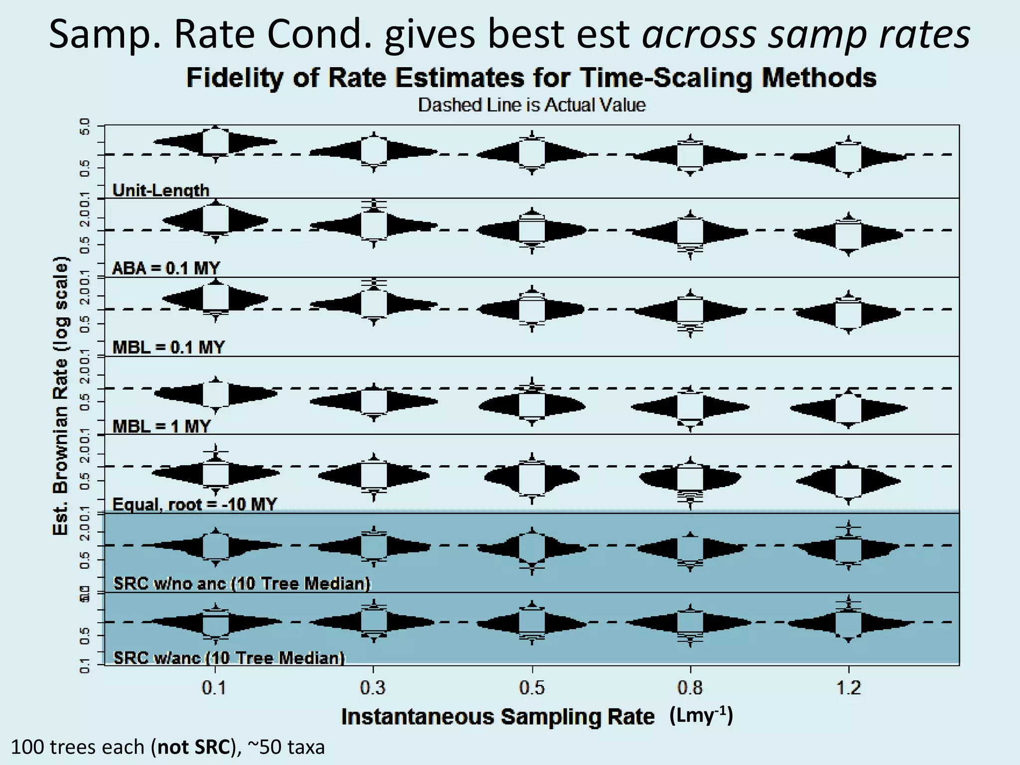
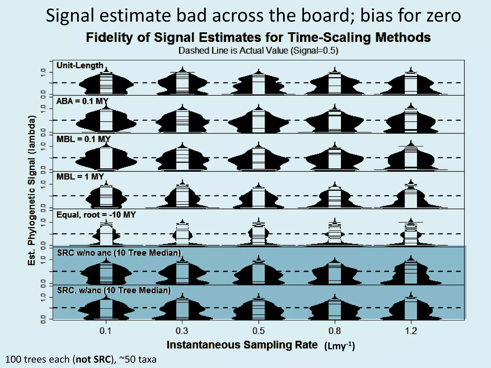
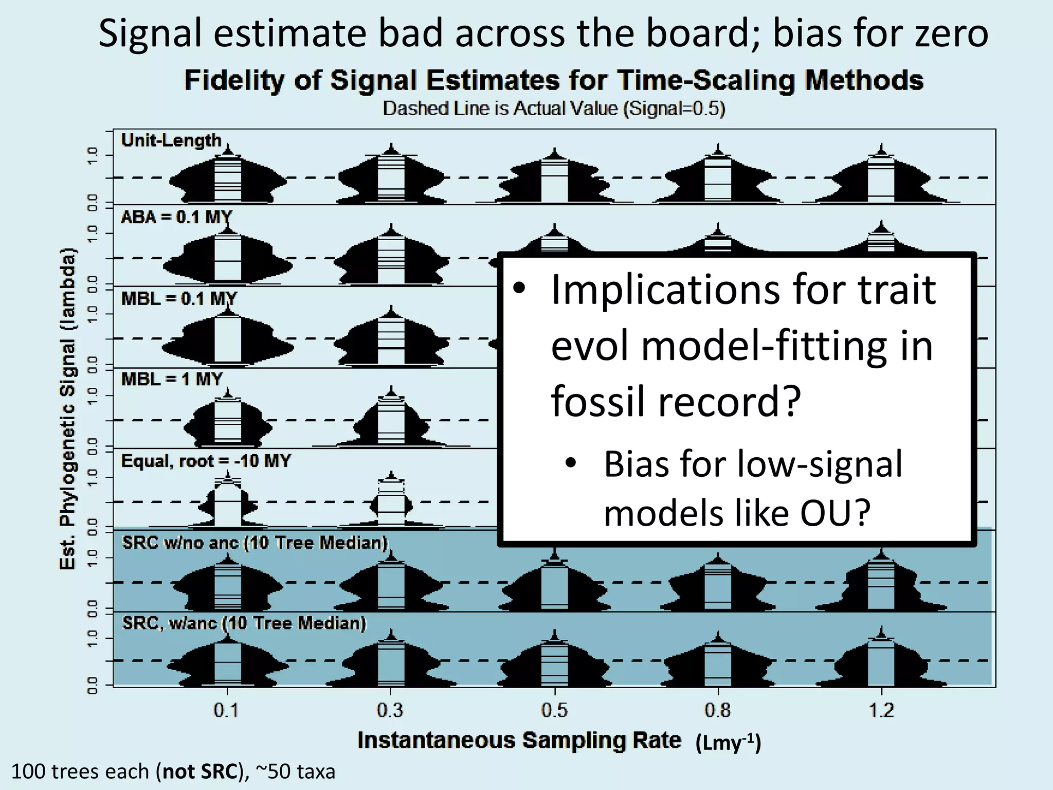
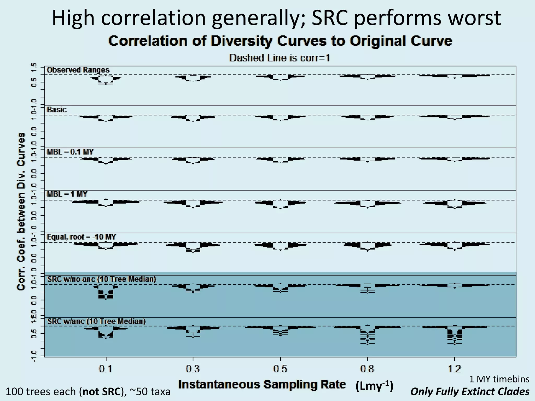
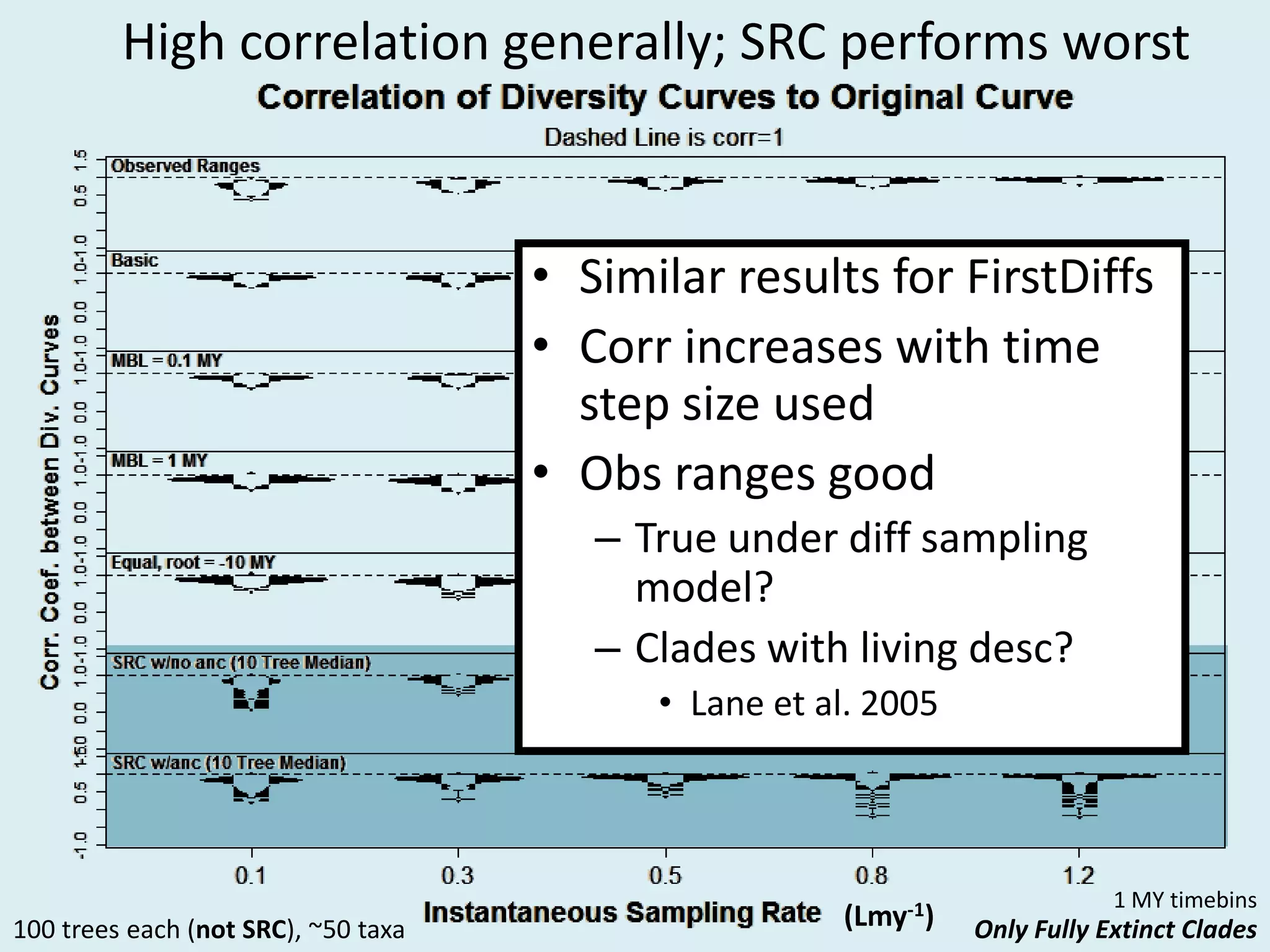
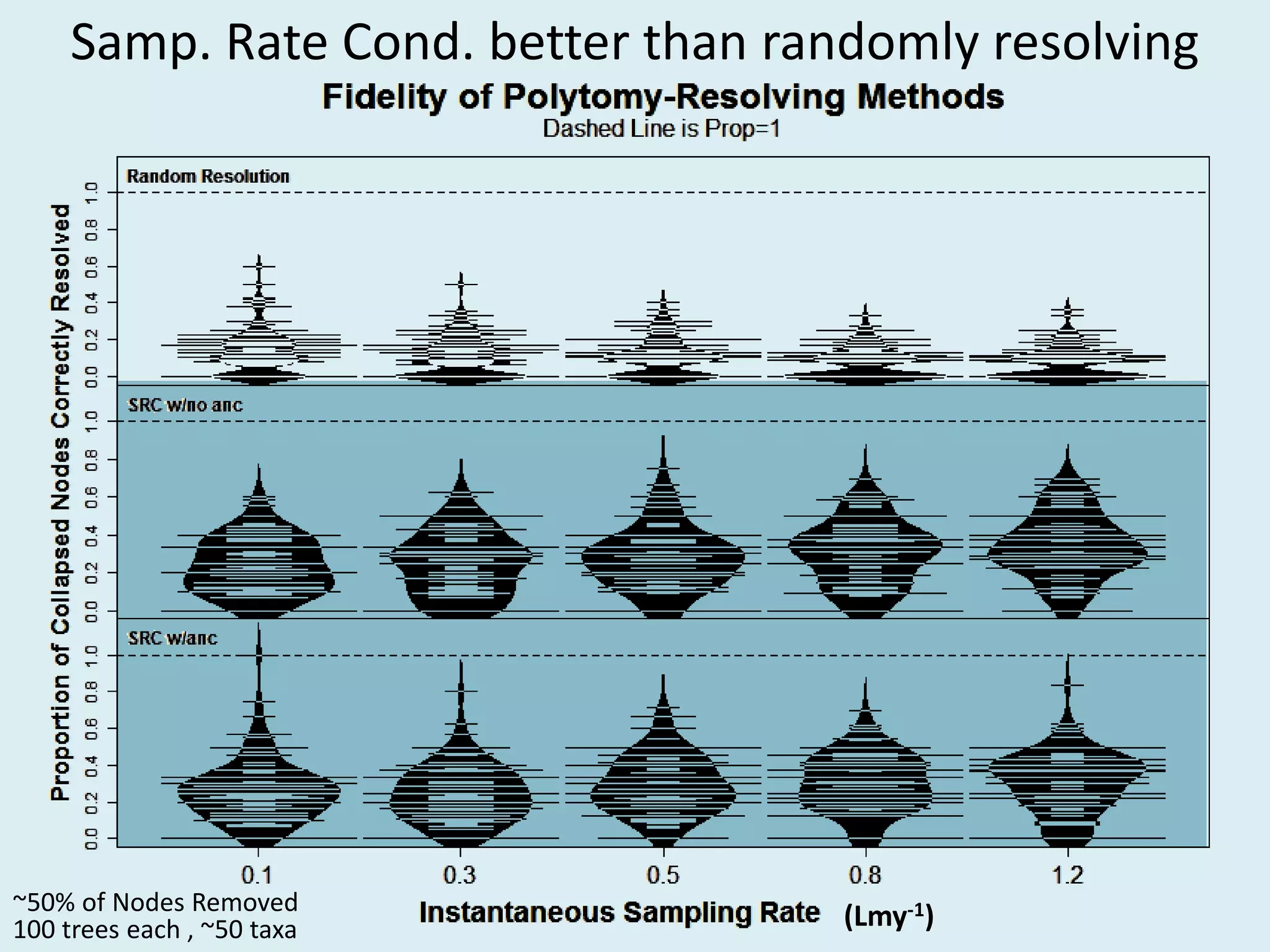
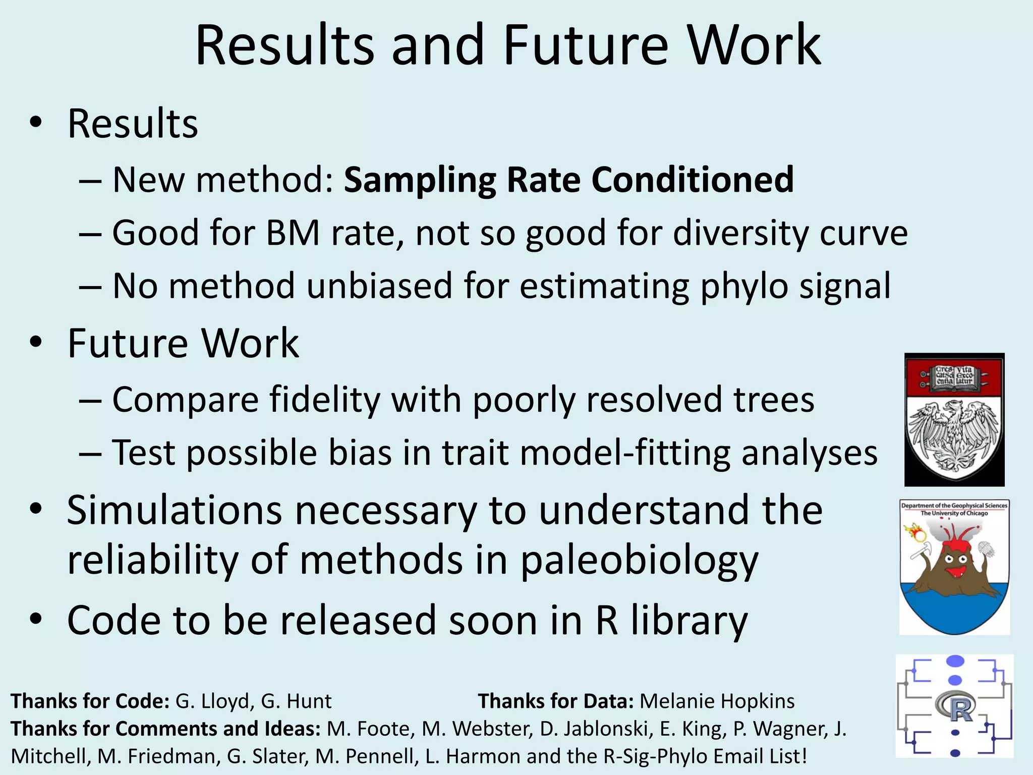


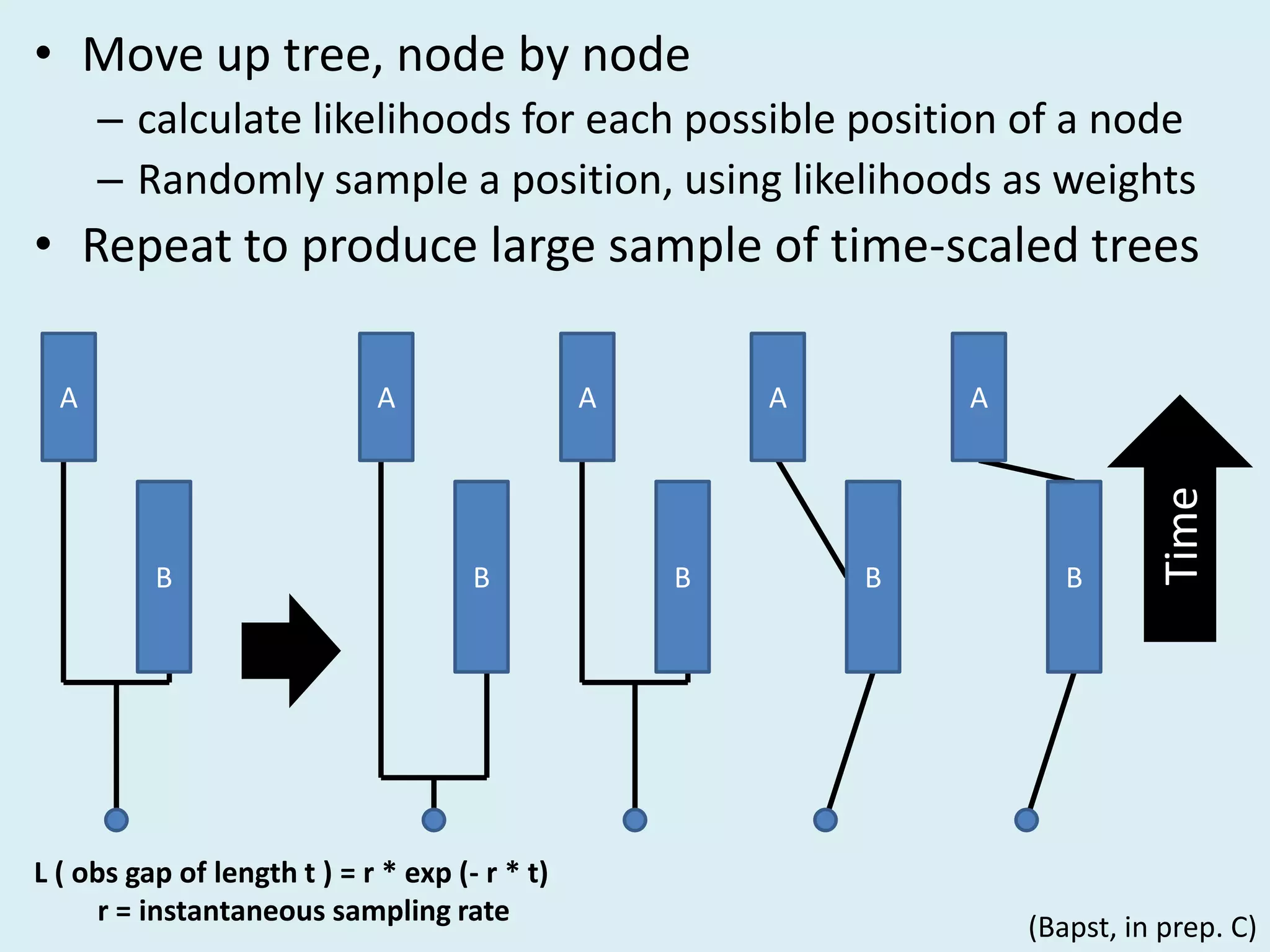
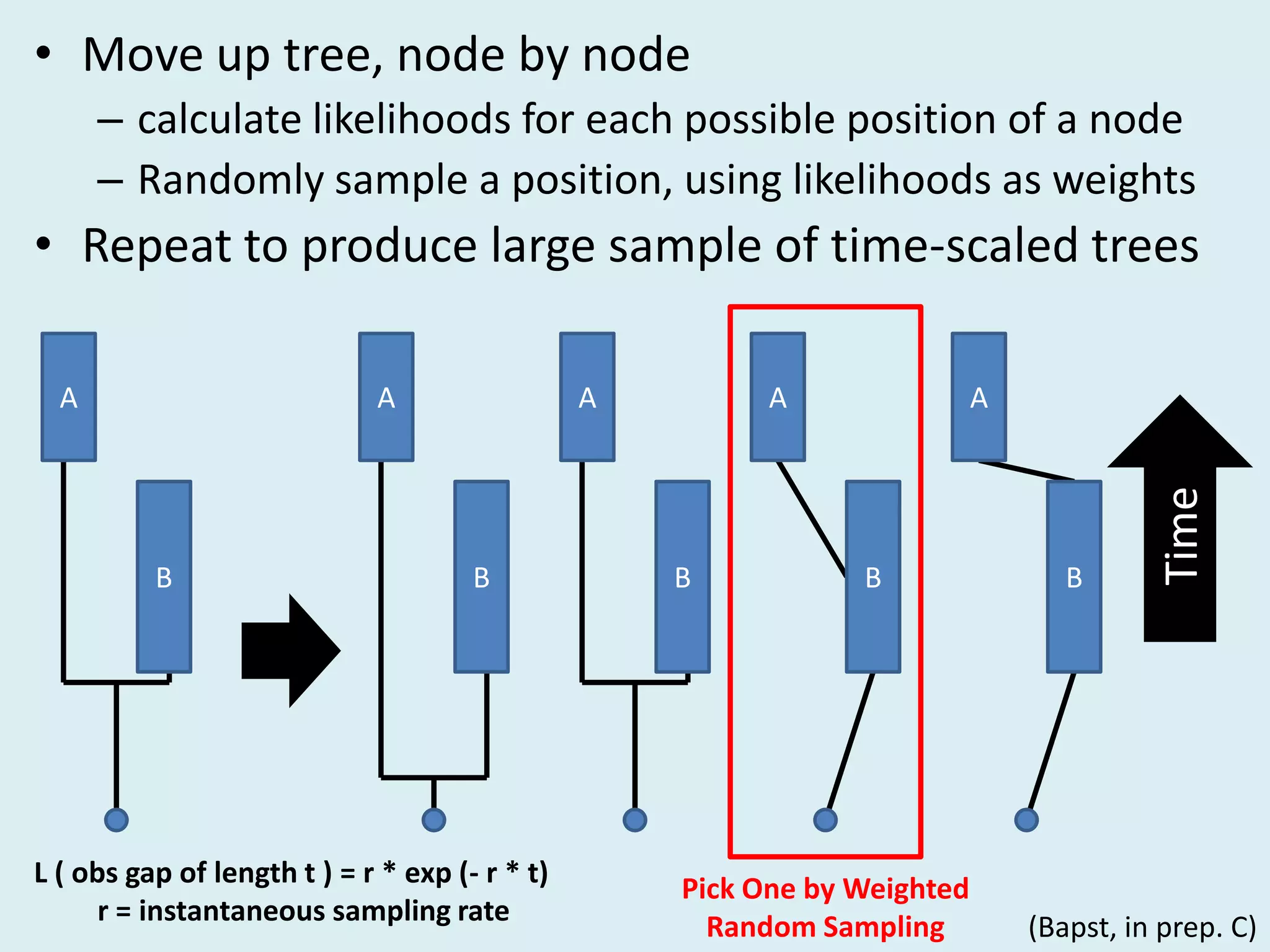
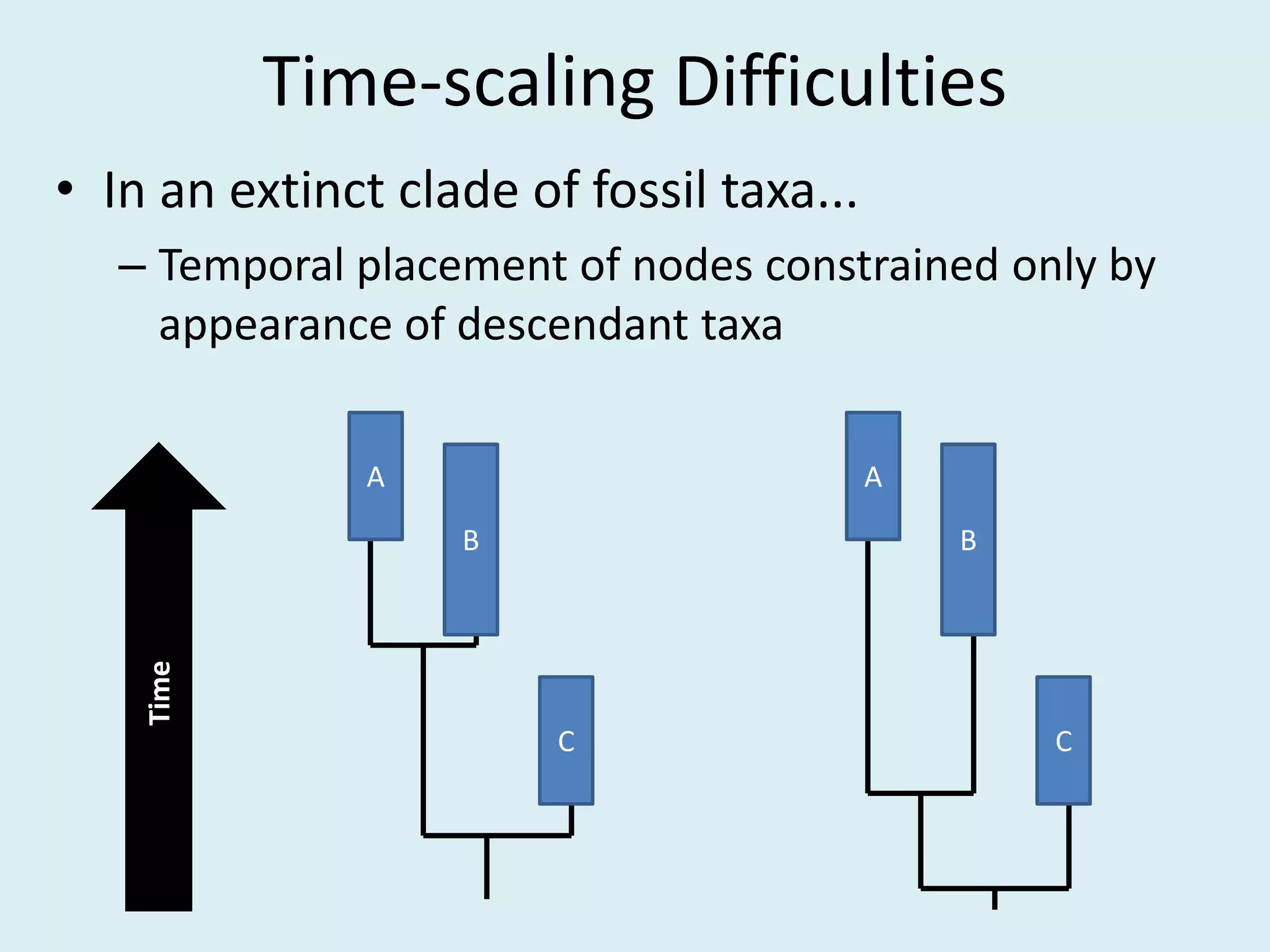
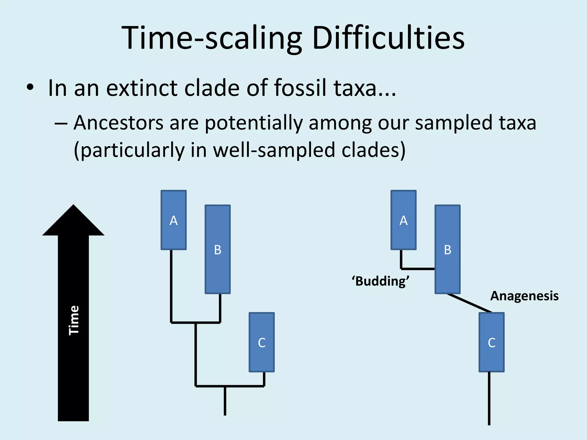
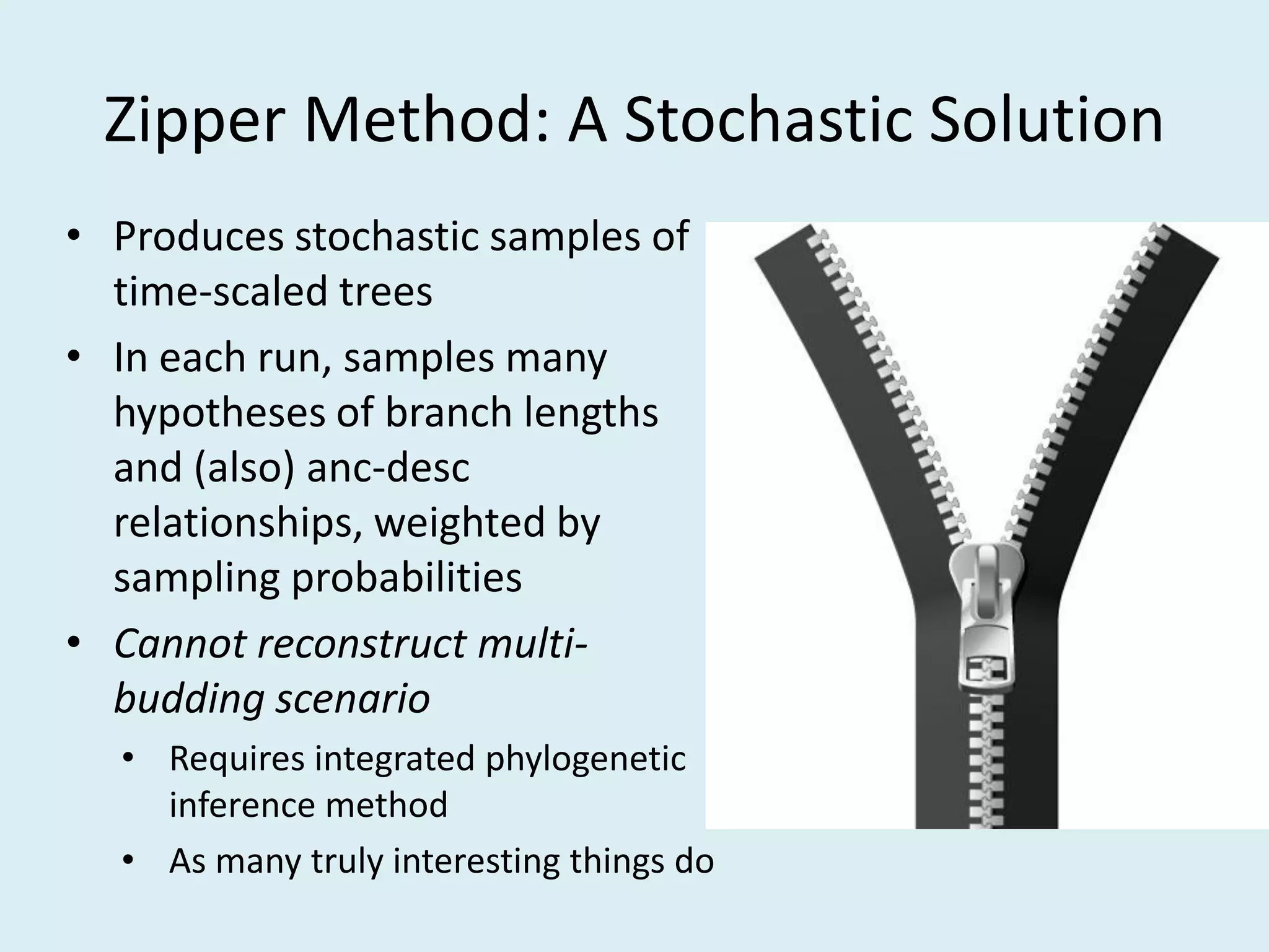
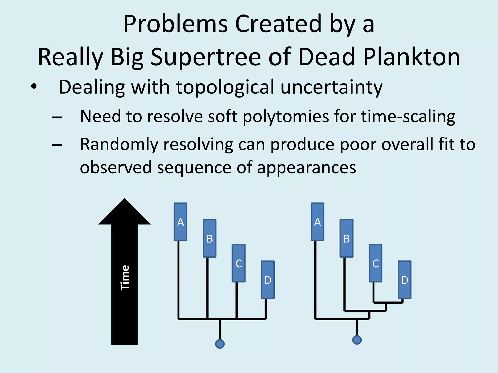

This document discusses various methods for time-scaling phylogenetic trees constructed from fossil occurrence data. It introduces a new method called sampling rate conditioned time-scaling that randomly scales branches based on the estimated fossil sampling rate to account for uncertainty. Simulation results show this method generally outperforms previous approaches in estimating divergence times, trait evolution rates, and model selection. Accounting for the incompleteness of the fossil record through probabilistic time-scaling methods improves analyses relying on time-scaled trees.


