The document provides analysis and interpretation of test scores for 30 candidates. It includes various graphs such as a pie chart, histogram, frequency polygon, ogive, scatter plot and measures of central tendency and variability. 1. The pie chart shows the distribution of scores, with most candidates scoring between 15-21 marks. 2. The histogram shows that most candidates (9) scored between 14.5-17.5 marks, indicating satisfactory overall performance. 3. Measures of central tendency - the mean score is 16.8, median is 16.5, and mode is 17 marks.

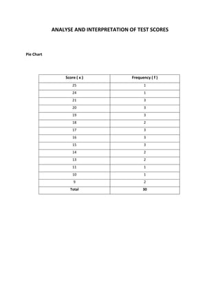
1. ANALYSE AND INTERPRETATION OF TEST SCORES
Pie Chart
Score ( x ) Frequency ( f )
25 1
24 1
21 3
20 3
19 3
18 2
17 3
16 3
15 3
14 2
13 2
11 1
10 1
9 2
Total 30

2. Pie Chart of 3 Dinamik Scores
25 24
10
11 3% 3%
13 3%
3%
7% 9
21
7%
10%
20
14
10%
7%
15 19
10% 10%
16 18
10% 17 7%
10%
The pie chart shows that:
1. 3% represents only 1 candidate who obtains 25 marks, 24 marks, 11 marks and 10 marks.
2. 7% represents 2 candidates who obtain 18 marks, 14 marks, 13 marks, and 9 marks.
3. 10% represents 3 candidates who obtain 21 marks, 20 marks, 19 marks, 17 marks, 16 marks and
15 marks.

3. Histogram
Class Interval Class Boundary Frequency
9 – 11 8.5 – 11.5 4
12 – 14 11.5 – 14.5 4
15 – 17 14.5 – 17.5 9
18 – 20 17.5 – 20.5 8
21 – 23 20.5 – 23.5 3
24– 26 23.5 – 26.5 2
Total 30
Histogram of 3 Dinamik Scores
10
9
8
7
Frequency
6
5
4
3
2
1
0
8.5 – 11.5 11.5 – 14.5 14.5 – 17.5 17.5 – 20.5 20.5 – 23.5 23.5 – 26.5
Scores

4. From the histogram, we can conclude that:
1. The score which most candidates obtained is 14.5-17.5.
2. The number of candidates who obtained the most scores within 14.5-17.5 is 9.
3. The total number of candidates who obtained sores within 17.5-20.5 is 8.
4. On the whole, the performance of the candidates is satisfactory because half of the candidates
obtained high marks.

5. Frequency Polygon
Class Interval Class Boundary Class Mark Frequency
9 – 11 8.5 – 11.5 10 4
12 – 14 11.5 – 14.5 13 4
15 – 17 14.5 – 17.5 16 9
18 – 20 17.5 – 20.5 19 8
21 – 23 20.5 – 23.5 22 3
24– 26 23.5 – 26.5 25 2
Total 30
Frequency Polygon of 3 Dinamik Scores
10
9
8
7
Frequency
6
5
4
3
2
1
0
0 8.5 – 11.5 11.5 – 14.5 14.5 – 17.5 17.5 – 20.5 20.5 – 23.5 23.5 – 26.5
Scores

6. Frequency Curve of 3 Dinamik Scores
10
9
8
7
Frequency
6
5
4
3
2
1
0
0 1 2 3 4 5 6 7
Scores

7. Ogive
Cumulative
Class Interval Upper Class Boundary Frequency
Frequency
9 – 11 11.5 4 4
12 – 14 14.5 4 8
15 – 17 17.5 9 17
18 – 20 20.5 8 25
21 – 23 23.5 3 28
24– 26 26.5 2 30
Ogive of 3 Dinamik Scores
35
30
25
Frequency
20
15
10
5
0
15
8.5 – 11.5 11.5 – 14.5 14.5 – 17.5 17.5 – 20.5 20.5 – 23.5 23.5 – 26.5
Scores

8. Percentage Ogive
Percentage
Upper Class Cumulative
Class Interval Frequency Cumulative
Boundary Frequency
Frequency
9 – 11 11.5 4 4 13.3
12 – 14 14.5 4 8 26.7
15 – 17 17.5 9 17 56.7
18 – 20 20.5 8 25 83.3
21 – 23 23.5 3 28 93.3
24– 26 26.5 2 30 100
Total 30
Percentage Ogive of 3 Dinamik Scores
35
30 100%
25
75%
Frequency
20
15 50%
10
25%
5
0
8.5 – 11.5 11.5 – 14.5 14.5 – 17.5 17.5 – 20.5 20.5 – 23.5 23.5 – 26.5
Scores

9. From the ogive, we can find that:
1. The number of candidates who failed, if the passing mark is 15 marks are 8 candidates.
2. The number of candidates who would obtain grade A, if grade A is 25 marks and above is only
one candidate.
Scatter plots
Score ( x ) Frequency ( f )
25 1
24 1
21 3
20 3
19 3
18 2
17 3
16 3
15 3
14 2
13 2
11 1
10 1
9 2
Total 30

10. Scatter Plots of 3 Dinamik Scores
3.5
3
2.5
Frequency
2
1.5
1
0.5
0
0 5 10 15 20 25 30
Scores
From the scatter plots, we can find that:
1. There are 3 groups of pupils: high, moderate and low performers.

11. MEASURES OF CENTRAL TENDENCY
Mean, Median and Mod
Class Interval ( x ) Class Mark ( x ) Frequency ( f ) (f)(x)
9 – 11 10 4 40
12 – 14 13 4 52
15 – 17 16 9 144
18 – 20 19 8 152
21 – 23 22 3 66
24– 26 25 2 50
Mean,

12. Median,
Where L = lower class boundary of median class
N= number of items in data
s= cumulative frequency of all classes prior to the median class
= frequency of median class
C= size of median class interval
Class Boundary Frequency Cumulative Frequency
8.5 – 11.5 4 4
11.5 – 14.5 4 8
14.5 – 17.5 9 17
17.5 – 20.5 8 25
20.5 – 23.5 3 28
23.5 – 26.5 2 30

13. Mode,
Where L = lower class boundary of modal class
= frequency of modal class – frequency before modal class
= frequency of modal class – frequency after modal class
C= class width
Class Boundary Frequency
8.5 – 11.5 4
11.5 – 14.5 4
14.5 – 17.5 9
17.5 – 20.5 8
20.5 – 23.5 3
23.5 – 26.5 2

14. Mode obtained from histogram :
Histogram of 3 Dinamik Scores
10
9
8 Mode
7
Frequency
6
5
4
3
2
1
0
17
8.5 – 11.5 11.5 – 14.5 14.5 – 17.5 17.5 – 20.5 20.5 – 23.5 23.5 – 26.5
Scores

15. MEASURES OF VARIABILITY
Range, Variance and Standard Deviation
Range = Highest Score – Lowest Score
= 25 – 9
= 16
Differences Squared,
Score ( x ) Differences,
25 25 – 16.8 = 8.2 67.24
24 24 – 16.8 = 7.2 51.84
21 21 – 16.8 = 4.2 17.64
20 20 – 16.8 = 3.2 10.24
19 19 – 16.8 = 2.2 4.84
18 18 – 16.8 = 1.2 1.44
17 17 – 16.8 = 0.2 0.04
16 16 – 16.8 = -0.8 0.64
15 15 – 16.8 = -1.8 3.24
14 14 – 16.8 = -2.8 7.84
13 13 – 16.8 = -3.8 14.44
11 11 – 16.8 = -5.8 33.64
10 10 – 16.8 = -6.8 46.24
9 9 – 16.8 = -7.8 60.84
Total = 232 Total = 320.16

16. Variance
=
=
=
Standard Deviation
=
=
=
=