
Recommended
Recommended
More Related Content
Recently uploaded
Recently uploaded (20)
Featured
Featured (20)
Data analysis 2 with Mathematica 10
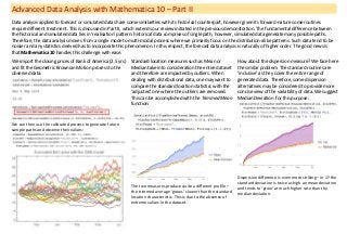
- 1. Advanced Data Analysis with Mathematica 10 – Part II Data analysis applied to forecast or simulated data share some similarities with its historical counterpart, however given its forward-nature some routines require different treatment. This is discussed in Part II, which extends our review initiated in the previous demonstration. The fundamental difference between the historical and simulated data lies in ‘realisation’ pattern: historical data comprises of single path, however, simulated data generate many possible paths. Therefore, the data analysis moves from a single mode to multi-modal process where we primarily focus on the distribution-alike patterns. Such data tend to be noisier and any statistics derived has to incorporate this phenomenon. In this respect, the forecast data analysis is naturally of higher order. The good news is that Mathematica 10 handles this challenge with ease. We import the closing prices of Bank of America (2.5 yrs) and fit the Geometric Brownian Motion process to the observed data: We can then use the calibrated process to generate future sample paths and observe their values: Standard location measures such as Mean or Median take into consideration the entire dataset and therefore are impacted by outliers. When dealing with distributional data, one may want to compare the standard location statistics with the ‘adjusted’ one where the outliers are removed. This can be accomplished with the Trimmed Mean function: The two measures produce quite a different profile – the trimmed average ‘grows’ slower than the standard location characteristic. This is due to the absence of extreme values in the dataset. How about the dispersion measure? We face here the similar problem. The standard routines are ‘inclusive’ as they cover the entire range of generated data. Therefore, some dispersion alternatives may be considered to provide more concise view of the variability of data. We suggest Median Deviation for this purpose: Dispersion difference is even more striking – in 1Y the standard deviation is twice as high an mean deviation and tends to ‘grow’ at much higher rate than the median deviation.
- 2. Mathematica 10 allows us to conduct the similar analysis in different order. Rather than working in ‘vertical’ dimension with distributed simulated data in a given point of time, we can change the order and work with data in the ‘horizontal’ direction first and then apply the ‘vertical’ aggregation. We replicate here the dispersion statistics with different ordering: 1) Turn stock prices into daily returns 2) Calculate the deviation along each path 3) Average the data The volatility and median deviation patterns are quite different – both numerically and in terms of patterns. Other useful measure of the dispersion in data is the inter-quartile range (I-Q range) that measures the distance between the two outermost quartiles. When the data is ‘spiky’, we can use the Mathematica’s function to identify the peaks in the data that exceeds certain thresholds. Here we again apply the higher-order analysis where we measure the I-Q range of the median in the projected stock prices for the next 12M (peaks >0.15 shown as black dots): Since all computed objects in Mathematica are internally consistent, we can work with them as with any other random variable. For example, I-Q range represents a certain distribution that we can examine and test further for detection of patterns. We compute the first two moments and check if the I-Q range is normally distributed: This does not look like a normal which is confirmed by the distribution fit test: