
Recommended
More Related Content
What's hot
What's hot (16)
Viewers also liked
Similar to Production & Operation Management Chapter5[1]
Similar to Production & Operation Management Chapter5[1] (20)
More from Hariharan Ponnusamy
More from Hariharan Ponnusamy (20)
Recently uploaded
Recently uploaded (20)
Production & Operation Management Chapter5[1]
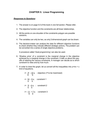
- 1. CHAPTER 5: Linear Programming Responses to Questions: 1. The answer is on page 5.5 of the book in one full section. Please refer. 2. The objective function and the constraints are all linear relationships. 3. All the points on one shoulder of the constraints polygon are possible solutions. 4. The variables can only be two, as only 2-dimensional graph can be drawn. 5. The decision-maker can analyze the data for different objective functions to check whether they indicate different strategic actions. The problem can be converted into a series of single objective problems. A procedure called ‘Goal programming’ can also be used. 6. ‘Shadow price’ of a constraint is the marginal change in the objective achieved by a marginal change in the constraint. It tells us about the pay- offs of relaxing the various constraints. A manager can decide as to which constraint to relax and by how much. 7. In order to draw the graph, let us convert all the inequalities into y=mx + c kind of equations. r= P - 10 q : objective ( P to be maximized) 9 9 r= 14 - 5 q : constraint 1 4 4 r= 9 - 4 q : constraint 2 5 5 r= - 11 + 7 q : constraint 3 9 9
- 2. 2 r 1 2 q 3 Obj. As seen above, constraints # 1 & 2 decide the values of the variables. Solving, we get: q= 0.265 and r=3.17 8. For a unique solution, it is necessary to have at least as many constraints as the decision variables. 9. Absolutely. In fact, the LP procedure ‘searches’ for the vertices of the n- dimensional polygon. Topology is very useful. 10.Dynamic programming is useful in situations where a series of interrelated (sequential) decisions are to be made. For example, in automobile production planning, monthly decisions may be made regarding how many cars of various models should be produced in each assembly plant. Optimal planning requires that enough cars be available to satisfy the highly seasonal and varying monthly demands and that this be achieved at a minimum cost. Or, a company may wish to make a series of marketing decisions over time which will maximize the sales volume. Each month’s production/sales level is a separate decision. However, each earlier choice affects the freedom of choice in later months. The decision one makes at each stage influences not only the next stage but also every stage to the end of the problem. Dynamic programming starts with the last stage of the problem and works backwards towards the first stage, making optimal decisions at each stage of the problem. Unlike in Linear programming, there is no ‘standard approach’ in Dynamic programming. It solves the large complex problem by breaking it down into a series of smaller problems which are more easily solved. The main advantage of Dynamic programming is its computational efficiency.
- 3. 3 11. Let the quantities (in ml) of shampoo and crème per girl per month be ‘s’ and ‘c’ respectively. The objective is to maximize the repel effect (E). Objective function: Maximize E = 2 s + 3 c. The constraints are for expenses per month per girl student, availability of the repellents Ugh & No-No, and the requirements of shampoo & crème per month. These are given below: 0.10s + 0.90 c ≤ 450 … (1) Money availability (0.011s + 0.005 c)(10) ≤ 15 …(2) Ugh availability (0.001s + 0.0025 c)(10) ≤ 5 … (3) No-no availability s ≥ (2) (10) (30) … (4) Shampoo requirement c ≥ (1) (10) (30) … (5) Crème requirement The LP is formulated and can now be solved using any software package. 12.Let M and S be the medical and surgical patients per month. We need to maximize total number of patients treated in a month. Objective function: Maximize Patients P = M + S. There are constraints on bed-days available, physio-days available, number of tests that can be done, number of X-Rays that can be taken and the number of surgical operations that can be performed in a month. These are expressed below. 7M + 3 S ≤ (100) (30) ….. (1) bed-days M + 2 S ≤ (25) (30) ….. (2) physio 10M + 5S ≤ (100) (30) …. (3) tests 5 M + 2S ≤ (36) (30) …. (4) X-rays S ≤ (10) (30) …. (5) surgeries Also, there are constraints on minimum medical and surgical cases that must be admitted per day. These are expressed below. S ≥ (5) (30) ….. (6) surgeries M ≥ (10) (30) ….. (7) medical cases The LP is now formulated and can be solved by graphical method or by using any software.
- 4. 4 CHAPTER 5: Linear Programming Objective Questions: 1. Shadow price in an LP problem is: √a. the coefficient of the slack variable. b. the idle capacity available within a constraint. c. the effect on the other objective function. d. the diseconomy of scale. 2. If there are three (3) decision variables, the constraints involving all three decision variables would be: a. lines √b. planes c. 3-dimensional cuboids d. n (more than 3)-dimensional figures. 3. The mathematical discipline that has much application in Linear Programming is: a. Probability theory b. Queuing theory c. Ontology √d. Topology 4. In Linear Programming (LP) what is optimized? a. Constraints √b. Objective function c. Decision variables d. Slack variables 5. Formulation of a Linear Programming problem consists of drawing up: a. Decision variables b. Constraints c. Objective function √d. All of the above 6. In an LP, inequities are used in: √a. constraints b. objective function c. a & b d. none of the above 7. Goal Programming can be useful when the optimization problem has: a. one specific or unique goal. b. goals instead of constraints. √c. multiple objectives.
- 5. 5 d. decision variables that cannot take fractional value. 8. For the case when the decision variable cannot take fractional values, a technique related to Linear Programming can be used. It is called: a. Goal programming b. Dynamic programming √c. Integer programming d. None of the above 9. Regarding decision variables, in a Linear Programming, it is assumed that: a. there are economies of scale. √b. there are no interactions between the decision variables. c. they are free to take any value. d. all of the above. 10.One of the pioneers in formulating the procedure of Linear Programming technique has been: √a. G.B. Dantzig b. Edward Deming c. Frederick W. Taylor d. Phil Crosby 11.Linear programming finds use in: a. Production planning b. Product-mix decisions c. Capital budgeting √d. All the above 12.When there are multiple objectives, we can use: √a. Goal programming b. Dynamic programming c. Integer programming d. None of the above 13.An iterative mathematical procedure used to solve a Linear programming problem is: a. Interpoint Savings method b. Kilbridge & Wester method c. Delphi method √d. Simplex method
- 6. 6 14.The following is a variant of Linear Programming: a. Bayesian analysis b. Strings & Weights analog method √c. Transportation problem d. None of the above 15.Simplex routine is basically a technique for:: √a. maximizing b. minimizing c. a & b d. none of the above 16.Strings & Weights method is used in: a. Purchasing √b. Warehouse location. c. Linear Programming d. Dynamic Programming 17.Transportation problem is related to: √a. Linear programming b. Purchase price decisions c. Inventory control under uncertainty d. Vehicle route scheduling 18.In Linear programming, the optimum solution lies: a. within the feasible region. b. in line with a binding constraint. c. in line with a slack constraint. √d. at one of the corners of the feasible region (polygon).