Production & Operation Management

1. Chapter 21: Inventory Models and Safety Stocks
Response to Questions:
1. Material delivery cost is relevant for procurement decisions such as:
“Where to source the supplies from?” For the purchasing manager,
material delivery cost is a ‘controllable’ cost. The number of deliveries, the
distance, and the type of the carrier or mode of transport are important
elements of the procurement cost.
2. Basic EOQ model is a static model and does not take into account the
uncertainties in either the demand or the supply of the item. It assumes a
constant rate of usage and in ‘lumpy’ demand situations this model is not
quite appropriate. The EOQ concept of ‘balancing’ various costs – such as
balancing the procurement costs and carrying costs – is a useful concept.
It could find use despite the model per se not being valid.
3. Changeover from one item to another in a manufacturing facility would
involve the cost of:
a) time spent in changing over,
b) rework, scrap, rejects during the setup and
c) paper work.
Costs (a) & (b) may be different for different sequences.
4. Yes, it would. One has to identify the least cost sequence in the joint
production run.
5. When product-runs are calculated individually, one assumes an ‘average’
set-up time, in an attempt to make the computations independent of the
sequencing decisions. Please note that inventory control calculations are
indeed based on several assumptions.
6. As mentioned in the earlier question, the set-up costs will differ for A, B
and C. The ‘joint cycle’ formula can be used without much difficulty.
7. The activities done before the material is procured and those done before
the material is processed are the cost generators. In manufacturing, the
cost is generated due to waiting of the plant/machinery/manpower. In
purchasing, the cost is generated mainly due to the various paperwork,
phone, fax, receipt and inspection activities. Thus, the components of the
cost are dissimilar. The similarity is that these are pre-manufacturing costs
and can be reduced to a bare minimum.
With proper technical action the manufacturing set-ups could be made
‘single touch’ setups; and with good supplier tie-ups and supply chains,

2. 2
the purchasing order costs could come down drastically. A batch can be
loaded immediately or a material can arrive just in time with minimal
ordering effort.
8. One of the components of carrying costs, viz. the capital cost, is amenable
to be expressed as a fraction of the value of the item. But, the other
components are not. Hence, expressing the carrying cost as a fraction of
the value of the item would not be an accurate way of computing the order
quantities. However, in any case, the ‘cost of capital’ itself is a nebulous
concept; and many simplifications exist in the inventory model itself.
Hence, expressing carrying cost as a fraction of the value of an item offers
much convenience adding only a little more to the existing simplification.
9. When a number of raw materials are procured:
(i) the difficulty is in apportioning order costs to the different
materials (How to divide telephone, follow up charges? How to
apportion effort?);
(ii) there is difficulty in also apportioning the space, materials
handling and insurance costs.
10. Aggregate inventory control can be done by using a Fixed Order Period
model. The carrying cost can also be expressed as a fraction of the value
of inventory.
11. Cost of not being able to fill an order is the shortage cost. However, there
are a number of ways in which a shortage can be met. The items could be
outsourced, borrowed, postponed, or staggered. Hence, computing the
shortage cost becomes difficult.
12. Stock-out can be expressed in terms of
(a) risk level: as done in the chapter, or in terms of
(b) shortage costs (explicit in money terms).
13. Safety stock is there to provide uninterrupted supply to the
production/operations, despite the vagaries in the supplies market and the
changes in the internal production demand.
14. Both R&M are needed simultaneously in order to make the product.
Service levels required = √ 95 / 100
= 0.9747 or 0.975
That is, a service level of 97.5% is required.

3. 3
15.In a fixed order quantity model, the correction (replenishment) takes place
after 1 lead time period. In fixed order period model, the correction takes
place only after a time period of (Lead time + Review period).
16.The fixed order cycle model is preferred when the order for the various
items is to be placed at the same time. This is convenient. However, the
safety stocks required are larger. Hence, the firm may prefer fixed order
quantity model.
17.The time between order and receipt is the ’lead time’. However, lead time
is not just the external (supplier’s) lead time. The internal lead time could
be as big as the external lead time and, hence, needs serious
consideration. How early the need should be communicated is the
question. Internal lead time involves the internal paper-work and other
communication to get the external ordering process started.
18. Inventory Control suggests generalized procedures, whereas Purchasing
and Physical Distribution functions could suggest response to specific
situations in the external market – when there is a dearth or a glut in the
market, when shipments are possible and when they are not. Hence, the
Purchase Manager and Manager of Logistics may want the Inventory
Control to be tempered by the realities of the external environment.
19.Inventory of materials is one type of operations capacity. Inventory could
give the firm the flexibility to respond to sudden demand surges. Hence,
carrying inventory is one of the operations strategies.
However, the other capacity-related strategies could include an ‘inventory’
of manpower, outsourcing and carrying back-orders. Manufacturing
strategies could relate to costs, agility, quality, timeliness, new
technologies etc. Thus, inventory is only a ‘part’ of the manufacturing
strategy.
20.The answer to this question is given in the previous response.
“Optimization of what?“ is the question that one needs to ask. Cost
optimization is not the only objective in front of the management of the
firm. Inventory models express one kind of efficiency and/or effectiveness
that is desired in the organization.
21.Inventory control, Purchasing, Manufacturing, Sales and Physical
Distribution are different aspects of management that need to be
integrated. These different activities need to be coordinated towards the
common organizational set of objectives.

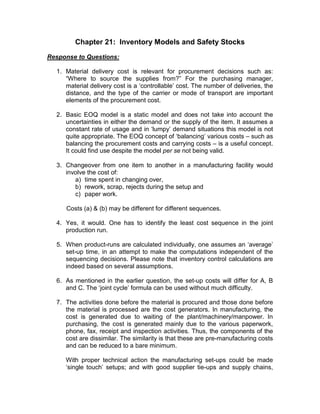
4. 4
22.Here Ku, the understocking cost, is the profit forgone, which is the
difference between sales price per unit and unit cost: (80p – 55p) = 25p.
Ko, the overstocking cost, is the loss in sale on the next day; which is the
difference between the cost per unit and the salvage value per unit: 55p –
40p = 15p.
F(x*) = Ku = 0.25 = 0.625
Ku + Ko 0.25 + 0.15
This is met at x = 700, where the cumulative probability is 0.650 slightly
exceeding the value 0.625.
Assuming that Iyengar makes buns only in 100’s, he should make 700
buns.
23.The service level is defined here in terms of 2 stock-outs in a year. This
necessitates that we know the number of ordering situations in a year.
Therefore, we need to find the EOQ for which the data is available.
EOQ = √ 2ACo
Cc
where A = annual demand = 52 x 1000 units
Co = Rs 200 per order
Cc = Rs 5 per unit
Therefore EOQ = √ 2X52000X200 = 2039.6 units
5
Number of ordering cycles per year A = 52000 = 25.5 = say 26.
Q 2039.6
∴ Service level is 26 -2 = 0.9231
26
This corresponds to a z value of 1.425 (this value is found by referring to
the Normal Distribution table given in Appendix II pg. 21.37)
Since the standard deviation of the usage during a week (which is also the
lead time) is 200 units, the safety stock required is:
(x - µ) = z.σ = 1.425 X 200 = 285 units

5. 5
This is shown in the Figure below.
24.p = 5,000 m/hr, r = 20,000/8 = 2,500 m/hr
A = (20,000 X 365) m/year
CO = 450 per set-up
Cc = 5x0.25 = Rs. 1.25 per m. per year
EBQ =
2 X 450 X (20000 x 365) = 1,02,528 m.
1.25 X (2500 / 5000)
No. of cycles required in a year = 20000 X 365 = 71.2 = 71 approx.
102528
If we make it 73 cycles, then the cycles are taken after every 5 days
(365/73 = 5).

6. 6
25. Solution : Q3opt = 2 x A x C0
s3 x f
where A = 10,000 C0 = Rs 300
f = 0.20 s3 = 9.70
Q3opt = 2 x 10000 x 300 = 1758.6
9.70 x 0.20
This quantity is in the middle price range and not in the range where price
s3 (i.e. Rs 9.70) prevails. Therefore, let us find Q2opt.
Q2opt = 2 x 10000 x 300 = 1745.2
9.85 x 0.20
This falls within its feasible range, because, for this quantity the price s2
(i.e. Rs 9.85) prevails. Refer to the following figure:
(TC)
T
o
t
a
l
c
o
s
t
s
Total cost vs Quantity Relationship for the Problem
The cost at Q2optimal = C0 . __A___ + s2 . f. Q2opt + (A . s2)
Q2opt 2

7. 7
= 300 x 10000 + 9.85 x 0.20 x 1745.2 + (10000 x 9.85)
1795.2 2
= 1719 + 1719 + 98,500 = Rs 1,01,938
We should compare the total costs at Q2opt with the total costs at b2 (i.e. second
price-break quantity).
Total costs at b2 = C0 . A + s3 .f. b2 + (A . s3)
b2 2
= 300 x 10000 + 9.70 x 0.20 x 300 + (10000 x 9.70)
3000 2
= 1000 + 2910 + 97000 = Rs 1,00,910
Therefore, TC (b2) < TC (Q2opt)
Thus, economic order quantity = b2 = 3000 units.
26.The problem is to:
Minimize 5 Qisi (1)
∑ 2
i = 1
(Note: Qisi/2 is the average stock value in Rupees for item ‘i’, Qi being the
order quantity, si, the price per unit of item ‘i’, and usage being assumed to
be uniform over time.)
The constraint is:
5 ai ≤ 10 (2)
∑ Qi
i = 1

8. 8
where ai = weekly usage of item ‘i’, in units.
Using λ as the Lagrange Multiplier, we define ‘F’ as:
5 Qisi + λ 5 ai _ 10
F = ∑ 2 ∑ Qi
i = 1 i = 1
Now, Equate ∂ F to zero and ∂ F to zero
∂ Qi ∂ λ
(i = 1, 2, …, 5)
On differentiation with respect to Qi we get, for each ‘i’:
si + λ . ai = 0
2 - Qi
2
Therefore Qi = 2λ . ai (3)
si
Now, 5 ai = 10 since ∂ F = 0
∑ Qi ∂ λ
i = 1
Substituting for Qi from Eq. (3):
5 ai . √si_ = 10 or 5 √ai si = 10
∑ √ (2λ . ai ) ∑ √(2λ)
i = 1 i = 1
Substituting the values of ai and si from the data given in the problem, we have:
1 √160x20 + √50x30 + √20x180 +√250x20 + √10x75 = 10
√(2λ)
Therefore, √λ = 17.92
Substituting the value of λ, now found, in Eq. (3):
Qi = 17.92 x 2ai …i = 1,2, …, 5
si
Thus, Q1 = 17.92 x 2x20 = 8.96 for Bushings
160
Q2 = 17.92 x 2x30 = 19.63 for Spl. Gaskets
50

9. 9
Q3 = 17.92 x 2x180 = 76.03 for Rings
20
Q4 = 17.92 x 2x20 = 7.17 for Seals
250
Q5 = 17.92 x 2x75 = 69.40 for Pins
10
The weekly orders, ni, are:
n1 = a1 = _20 = 2.23
Q1 8.96
n2 = _30 = 1.53
19.63
n3 = _180 = 2.37
76.03
n4 = _20 = 2.79
7.17
n5 = _75 = 1.08
69.40
Rounding off to the nearest possible integer, we have:
n1 = 2 (for Bushings)
n2 = 2 (for Special Gaskets)
n3 = 2 (for Rings)
n4 = 3 (for Seals)
n5 = 1 (for Pins)
∑ni = 10
The above values give the scheme of ordering for VACO.
The order sizes would, therefore, be:
_______________________________________________________
Serial No. Item No. of Orders Order Size (units)
1. Bushings 2 10
2. Spl. Gaskets 2 15
3. Rings 2 90
4. Seals 3 7, 7 and 6
5. Pins 1 75_______

10. 10
Alternative Solution:
A simple intuitive-cum-trial-&-error approach to the solution of the above problem
could also have been attempted. Such an approach may be allowed here, since
in the earlier solution the number of orders was approximated to the nearest
possible integer. Otherwise, the method involving Lagrange multiplier is quite
precise in calculating the optimal quantities.
The simplistic approach is as follows:
1. Compute the weekly usages of the items in Rupee values.
2. Find the total weekly usage of all the five items; compute the average
Rupee value per order, if 10 (maximum allowed) orders were placed.
3. It is intuitively expected that if the number of orders of each item is
calculated on the basis of average Rupee value per order (earlier
computed), the solution would be optimal or near-optimal.
4. The average stock value (in Rs) is calculated for the above solution.
5. Slight changes may be made in the number of orders for the items and
it may be checked as to whether the average stock value goes any
further down.
6. Accordingly the desired trial-&-error changes are made.
7. The minimum (average stock value) gives the optimal solution.
The computations are given below. The following table gives the first intuitive
values for the number of orders.
No. of Orders Average Stock
Sl Price per Weekly Weekly to be placed= Value
No. Item Unit Usage Usage (Weekly Usage) (Rupees)
(Rs) (units) (Rupees) (1205)
1. Bushings 60 20 1200 1 1200 = 600
1 x 2
2. Spl. Gaskets 50 30 1500 1 1500 = 750
1 x 2
3. Rings 20 180 3600 3 3600 = 600
3 x 2
4. Seals 250 20 5000 4 5000 = 633
4 x 2
5. Pins 10 75 750 1 750 = 375
1 x 2
Total = 12,050 Total = 10 Total = 2958
Average per order = 12,050 = 1,205
10

11. 11
The next set of computations try values which are slightly different from the above.
Trial No. 2 Trial No. 3
Sl Weekly No. of Orders Average No. of Orders Average Stock
No. Item Usage per Week Stock Value per Week Value
(Rupees) (Rupees) (Rupees)
1. Bushings 1200 1 600 2 300
2. Spl. Gaskets 1500 2 375 2 375
3. Rings 3600 3 600 2 900
4. Seals 5000 3 833 3 833
5. Pins 750 1 375 1 375
Total = 2783 Total = 2783
It is noted that both the trials give the same average stock value which is lower
than that found in Trial No. 1. We take one of the latter trial values (of the order
sizes) as our solution. It may be noted that trial No. 3 gives the same solution as
found by the use of Lagrange multiplier earlier.

12. 12
CHAPTER 21: Inventory Models and Safety Stocks
Objective Questions
1. Basic EOQ model assumes:
a. Order quantity is fixed
b. Rate of usage of the material is constant
√c. a & b
d. none of the above
2. When usage is varying, the basic EOQ model needs coverage (by means
of a safety stock) over :
√a. one lead time.
b. a period of time computed based upon the desired service level.
c. one standard deviation of the lead time.
d. none of the above.
3. In a ‘two-bin’ system, one of the bins is stocked equal to:
a. normal usage over the review period.
b. normal usage over the review-plus-lead time.
√c. normal usage over the lead time.
d. none of the above.
4. Re-order Point, in the absence of buffer stocks, equals:
√a. normal usage over one lead time.
b. normal usage over a review period.
c. normal usage over one lead time plus one review period.
d. none of the above.
5. For the same normal usage rate and the same lead time, which of the
following is true?
a. Q-system needs more buffer stock than the P-system of inventory
control.
b. Q-system and P-system need the same level of buffer stock.
√c. Q-system needs less buffer stock than the P-system.
d. none of the above.
6. Usage rate is 100 items per day, procurement cost is Rs. 2000 per
procurement order, the lead time is 4 days and the cost of carrying
inventory is 25 per cent. Each item costs Rs. 400. If a month is taken to
have 30 days, the economic order quantity in this case is:
a. 400
b. 800
√c. 1200
d. data inadequate

13. 13
7. For the above question (Question No.6) the safety stock, corresponding to
an enhanced usage level of 200 items per day, is:
√a. 400
b. 800
c. 1200
d. none of the above
8. Guru Provisions buy an item worth Rs.1 lakh. The inventory carrying costs
are 25 per cent and each ordering procedure involves an expenditure of
Rs. 500. How many orders should Guru place in a year?
a. 2 b. 3 c. 4 √d. 5
9. India Soaps Limited (ISL) buys 1000 tons of tallow annually. The cost of
carrying is estimated at 30 per cent and order cost is estimated at Rs.
10,000 per order. Price of tallow in the supply market is Rs. 10,000 per
ton. Allowing for an annual inflation of 20 per cent in the tallow prices,
what should be ISL’s optimal order quantity for tallow?
a. 105.5 tons
b. 122.4 tons
√c. 148.5 tons
d. 81.6 tons
10.Out of 400 orders, the 372 which were met were all for one unit each;
while the 28 which were not met, were all for five units each. The service
level, in this case, may be said to be:
a. 93 per cent
b. 72.7 per cent
c. 65.8 per cent
√d. either 93 per cent or 72.7 per cent depending upon the definition of
service level.
11.When usage rate variation is probabilistic – approximated to a normal
distribution, if the lead time increases from 1 month to 2 months, the
safety stock requirements will increase by:
√a. 41.4 %
b. 50 %
c. 70.7 %
d. 100 %
12.In a P-system of inventory control, the maximum inventory on hand plus
on order is equal to:
a. Buffer stock.
b. Order quantity plus average usage over lead time.
√c. Average usage over a review period-plus-lead time plus buffer
stock.

14. 14
d. Buffer stock plus average usage over a review period.
13.SNC–ZXLQ brand of radial tyres have a procurement lead-time of 2
weeks, a weekly usage rate of 40 units and a weekly standard deviation of
10 units. Assuming a Normal probability distribution, for a 97 per cent
service level what is the reorder point for this tyre?
a. 60
b. 67
c. 80
√d. 107
14. In the inventory model with purchase discount, the optimal quantity is
Q2 optimal (i.e. that corresponding to Price 2) if:
a. Q2 optimal is higher than Q1 optimal
b. Q2 optimal falls in the zone of Price 1
√c. Q2 optimal falls in the zone of Price 2
d. none of the above