Running Head: Week 3 – Assignment 1: Demand Estimation 1
Assignment 1: Demand Estimation
Ray W. Vance
Strayer University
ECO 550– Managerial Economics and Globalization
Doctor Mohammad Sumadi
Oct 23, 2016
MY INTRODUCTION
This is a report about Demand Estimation. Demand estimation is a proven method of estimating all future sales that a company will make. It is crucial in determining decisions that are vital to the firm. Demand Estimating employs calculations which are acquired on price elasticities, income elasticities, cross price elasticities, and advertisement elasticities, to provide decisive information relative to the firm's expectations, of forthcoming market sales. It is essential for a company to know decisively, if it should increase, or cut it's prices of the goods they sell, contingent on the conditions of the market. Additionally, the firm needs to know, which factors will affect these changes, in both the quantity demanded, as well as the quantity supplied always.
Demand Estimation
The elasticity of demand, indicates the relationship between changes in quantity, demanded changes, and the price changes. Price sensitivity issues are a challenge to every organization, that operates in a competitive environment. Organizations must make considerations for the elasticities, since they enable them to make a forecast, of any changes in the demand for their products. They also imply an impact of the changes, in the prices of the products, and other essential market factors. A firm will be able to make the needed adjustments, to ensure that it maximizes the revenue for the business.
Elasticities For Each Independent Variable
Option 1
QD = - 5200 - 42P + 20PX + 5.2I + 0.20A + 0.25M
(2.002) (17.5) (6.2) (2.5) (0.09) (0.21)
R2 = 0.55 n = 26 F = 4.88
Substituting the values from the values given above,
QD = - 5200 - 42P + 20PX + 5.2I + 0.20A + 0.25M
P= 500, PX=600, I= 5500, A= 10,000, M= 5,000
QD = - 5200 – 42(500) + 20(600) + 5.2 (5,500) + 0.20(10,000) + 0.25(5000)
QD= 17,650
Price Elasticity= (P/Q) * (dQ /dP)
From the regression equation, (dQ/dP) = -42, the price of the widget
Thus, price elasticity= (500/17650) *(-42) = -1.19
The Cross Price Elasticity, EPX= (600/17650)*20= 0.68
Also, the Income Elasticity, EI= (5500/17650) *5.2= 1.62
Advertisements Elasticity, EA = (10,000/17650) *0.20= 0.11
Micro-Oven elasticity, EM= (5000/17650) *0.25= 0.07
Implications Of The Above Computed Elasticities For The Business In Terms Of Short-Term And Long-Term Pricing Strategies
Price Elasticity, -1.19
Since the price elasticity is negative, it implies that with a 1% increase in t ...
Unit-IV; Professional Sales Representative (PSR).pptx
Running Head Week 3 – Assignment 1 Demand Estimation .docx
1. Running Head: Week 3 – Assignment 1: Demand Estimation
1
Assignment 1: Demand Estimation
Ray W. Vance
Strayer University
ECO 550– Managerial Economics and Globalization
Doctor Mohammad Sumadi
Oct 23, 2016
MY INTRODUCTION
This is a report about Demand Estimation. Demand
estimation is a proven method of estimating all future sales that
a company will make. It is crucial in determining decisions that
are vital to the firm. Demand Estimating employs calculations
which are acquired on price elasticities, income elasticities,
cross price elasticities, and advertisement elasticities, to
provide decisive information relative to the firm's expectations,
of forthcoming market sales. It is essential for a company to
know decisively, if it should increase, or cut it's prices of the
goods they sell, contingent on the conditions of the market.
Additionally, the firm needs to know, which factors will affect
these changes, in both the quantity demanded, as well as the
quantity supplied always.
Demand Estimation
The elasticity of demand, indicates the relationship between
changes in quantity, demanded changes, and the price changes.
Price sensitivity issues are a challenge to every organization,
that operates in a competitive environment. Organizations must
make considerations for the elasticities, since they enable them
2. to make a forecast, of any changes in the demand for their
products. They also imply an impact of the changes, in the
prices of the products, and other essential market factors. A
firm will be able to make the needed adjustments, to ensure that
it maximizes the revenue for the business.
Elasticities For Each Independent Variable
Option 1
QD = - 5200 - 42P + 20PX + 5.2I + 0.20A + 0.25M
(2.002) (17.5) (6.2) (2.5) (0.09) (0.21)
R2 = 0.55 n = 26 F = 4.88
Substituting the values from the values given above,
QD = - 5200 - 42P + 20PX + 5.2I + 0.20A + 0.25M
P= 500, PX=600, I= 5500, A= 10,000, M= 5,000
QD = - 5200 – 42(500) + 20(600) + 5.2 (5,500) + 0.20(10,000)
+ 0.25(5000)
QD= 17,650
Price Elasticity= (P/Q) * (dQ /dP)
From the regression equation, (dQ/dP) = -42, the price of the
widget
Thus, price elasticity= (500/17650) *(-42) = -1.19
The Cross Price Elasticity, EPX= (600/17650)*20= 0.68
Also, the Income Elasticity, EI= (5500/17650) *5.2= 1.62
Advertisements Elasticity, EA = (10,000/17650) *0.20= 0.11
Micro-Oven elasticity, EM= (5000/17650) *0.25= 0.07
Implications Of The Above Computed Elasticities For The
Business In Terms Of Short-Term And Long-Term Pricing
Strategies
Price Elasticity, -1.19
Since the price elasticity is negative, it implies that with a 1%
increase in the prices of the product, the quantity demanded
3. drops by 1.19%. The increase in the price, has a small impact on
the change in demand, thus it can be referred to as somehow
elastic. The decrease in the demand, thus is not entirely
contributed, by the change in prices. Nonetheless, any increase
in price, will still drive some customers away. It will also
depend with the market share. If the market share is high, the
customer base may be lost to a higher extend (Baumol, &
Blinder, 2015).
Cross Price Elasticity, 0.68
Cross Price Elasticity, measures the responsiveness of the
demand of an organization’s goods, relative to that of the
competitor. Thus, a cross price elasticity of 0.68, indicates that
if the price of the competitor’s product increases by 1%, the
quantity demanded increases by 0.68%. Thus, the product is
fairly elastic, in comparison to the competitor’s price. The price
of the competitor, does not have an impact on sales of the
organization.
Income Elasticity, 1.62
An income elasticity of 1.62, implies that a 1% increase in the
average income of individuals, results in an increase in the
quantity demanded by 1.62%. The product is thus elastic. The
management can make a consideration of increasing the price of
the product, if the average income increases.
Advertisements Elasticity, 0.11
An advertisement elasticity of 0.11, implies that a 1% increase
in the advertising expenses, will result in an increase in the
quantity demanded by 0.11%. The demand for the product is
elastic to the advertising expenses. Even with more
advertisement, it does not imply that the company could venture
into increasing prices, since this could drive customers away.
Micro-Oven Elasticity, 0.07
A micro-oven elasticity of 0.07 implies that a 1%
increase in the number of ovens, will result in an increase in the
quantity demanded, by only 0.07%. The demand for the micro-
oven is inelastic.
Therefore, the quantity demanded is sensitive to the price of the
4. product, and the average income of individuals. However, the
quantity demanded is insensitive to the prices of the
competitor’s price. It is also noted that the quantity demanded,
is insensitive to advertising and the amount of the microwaves
in the market.
Recommendations On Whether I Believe The Firm Should, Or
Should Not, Cut Its Price To Increase Its Market Share
The price elasticity is -1.19%. Thus, the firm should cut its
price to increase its market share. A decrease in the price of the
product, results in an increase in the quantity demanded. When
the elasticity of product is one, an organization should try to
maximize its revenue. Thus, a decrease in the price, results in
an increase in the quantity demanded. The net result is an
increase in the sales, thus increasing its market share, and the
revenue that is generated (Case, Fair, & Oster, 2014).
Assume that the price changes are 100, 200, 300, 400, 500, 600
cents
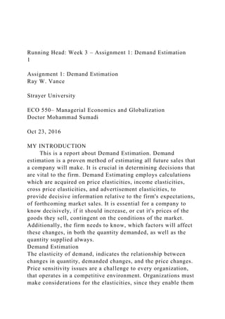
Demand Curve For The Firm:
QD = - 5200 - 42P + 20PX + 5.2I + 0.20A + 0.25M
Substituting the values,
Q = -5200 - 42*P + 20*600 + 5.2*5500 + 0.2*10000 +
0.25*5000
Q = 38650 - 42P
P= 38650/42-Q/42
Price
Quantity Demanded
100
34450
200
30250
300
26050
400
21850
6. P = 384.478
Equilibrium price= 384.478
At equilibrium= Q= -7909.89+79.1(384.478) = 22502.3198
Thus, Q= 22,502 units
In the below curve, the point at equilibrium is where the
demand curve, and supply curve intersect.
Relevant Factors That Cause Changes In Supply And Demand
For Low-Calorie, Frozen Microwavable Food, And the Method,
In Both Short-Term And Long-Term Changes, In Market
Conditions, That Impact The Demand For, And The Supply Of
The Product
From the elasticities calculated above, the demand for
the low-calorie, frozen microwavable food, is affected by the
changes in the average consumer income, and competitor’s
price, and the prices of the related goods, the microwavable
oven. Consumer preferences also impact the quantity demanded.
Some consumers have an increased awareness, towards the low-
calorie foods, thus affecting the amounts of the product
demanded (Case, Fair, & Oster, 2014).
On the other hand, the supply of the low-calorie, frozen
microwavable food, is affected by the changes in the number of
the suppliers of the product. Any technological advances in the
production of the product, may also impact the quantity
supplied. Also, the availability of labor and the raw materials
used in the production of the product, have an impact on the
quantity supplied. It is due to the fact that they have a direct
effect, on the costs of production of the product(Hall, &
Lieberman, 2012).
Crucial Factors That Cause Rightward Shifts And Leftward
Shifts Of The Demand And Supply Curves For The Low-
Calorie, Frozen Microwavable Food
7. Crucial factors that cause rightward shift in the demand curve,
include the increase in the average consumer income, and even
a decrease in prices of complementary products. Increase of
consumer preferences, also result in a rightward shift of the
demand curve. Increase of the consumer preferences towards the
product, may be attributed to an increase in the awareness of the
low calorie foods. On the other hand, a leftward shift in the
demand curve, could be as a result of a decrease in the
consumer’s income, or an increase in a complementary
product’s price (Hall, & Lieberman, 2012).
Crucial factors that result in a leftward shift in the
supply curve, include the availability of cheap labor,
technological advancements in the production of the product,
and a decrease in taxation. These are all results of the decrease,
in the cost of production. There may be an availability of
abundant raw materials, resulting in the production of a lot of
goods to be supplied. On the other hand, left-ward shift in the
supply curve, may be caused by a scarcity of raw materials, and
increase in taxation. Increase in the rates of interest, and an
increase in the worker’s wages, result in the leftward shift in
the supply curve(Hall, & Lieberman, 2012).
CLOSE
OK, so this was a report regarding Demand Estimation.
Yes, demand estimation is a proven method of estimating all
future sales, that a company makes. It is crucial indeed, in
determining decisions vital to the firm. Demand Estimating
employs calculations acquired on price elasticities, income
elasticities, cross price elasticities, and advertisement
elasticities, to provide decisive information, related to the
firm's expectations, of forthcoming market sales. It is vital for a
company to know concisely, if it should increase, or cut it's
prices of goods sold, contingent on the market's conditions.
Additionally, the firm needs to know, what factors affect those
changes, in both the quantity demanded, and the quantity
supplied at all times. That said, let's go over the latest numbers,
to develop tomorrow's expected forecast.
8. References
Baumol, W., & Blinder, A. (2015). Microeconomics: Principles
and policy. Cengage Learning. Retrieved Oct. 23, 2016.
Case, K. E., Fair, R. C., & Oster, S. (2014). Principles of
microeconomics. Pearson Higher Ed. Retrieved Oct. 23, 2016.
Hall, R., & Lieberman, M. (2012). Microeconomics: Principles
and applications. Cengage Learning. Retrieved Oct. 23, 2016.
_292754564.xls
Chart1344503025026050218501765013450
P
Demand Curve
100
200
300
400
500
600
Sheet1Tasks/TaskTime
(mininutes)BROPNEPHASINAggregateCheck-
In3030303030Evaluation2015101213.4259259259Testing45401
51524.7222222222Assessment1515101011.7592592593Total
Work Content110100656779.9074074074AVERAGE
PATIENTS PER DAYBROPNEPHASINPatients /
Day20183040Fraction of
total0.18518518520.16666666670.27777777780.37037037041
Sheet2IF Individual Products madeProductPriceWorker1
(min)Worker2(min)Total Time(hrs)material costlabor
cost/unitProfit MarginConstraint Tme (hrs)units/hrTotal units in
dayRevenue/dayLabor costs/dayMaterial
costs/dayProfits/dayW5635200.9162013.7422.260.5831.715265
866213.7221269297768.4391080617240274.4425385935253.99
65694683X5530200.8332512.49517.5050.5216880240400240Y5
420350.9162513.7415.260.5831.715265866213.7221269297740.
9948542024240343.0531732419157.9416809605Z5310350.7520
11.2521.750.5831.715265866213.7221269297727.27272727272
9. 40274.4425385935212.8301886792ProductPriceWorker1
(min)Worker2(min)Total Time(hrs)material costlabor
cost/unitProfit Marginunits per hrunits per
dayRevenues/dayLabor costs per dayMaterial
costs/dayProfits/dayW5635200.9162013.7442.261.09170305688
.7336244541489.0829694323240174.67248908374.4104803493
X5530200.8332512.49542.5051.20048019219.6038415366528.2
112845138240240.096038415448.1152460984Y5420350.916251
3.7440.261.09170305688.7336244541471.615720524240218.34
0611353713.2751091703Z5310350.752011.2541.751.333333333
310.6666666667565.3333333333240213.3333333333112
Sheet3
Sheet4QP344501003025020026050300218504001765050013450
600
Sheet4
P
Demand Curve
· Week 3 Assignment
Students, please view the "Submit a Clickable Rubric
Assignment" in the Student Center.
Instructors, training on how to grade is within the Instructor
Center.
Assignment 1: Demand Estimation
Due Week 3 and worth 200 points
Imagine that you work for the maker of a leading brand of low-
calorie, frozen microwavable food that estimates the following
demand equation for its product using data from 26
supermarkets around the country for the month of April.
For a refresher on independent and dependent variables, please
go to Sophia’s Website and review the Independent and
Dependent Variables tutorial, located at
http://www.sophia.org/tutorials/independent-and-dependent-
variables--3.
10. Option 1Note: The following is a regression equation. Standard
errors are in parentheses for the demand for widgets.
QD = - 5200 - 42P + 20PX + 5.2I + 0.20A + 0.25M
(2.002) (17.5) (6.2) (2.5) (0.09) (0.21)
R2 = 0.55 n = 26 F = 4.88
Your supervisor has asked you to compute the elasticities for
each independent variable. Assume the following values for the
independent variables:
Q = Quantity demanded of 3-pack units
P (in cents) = Price of the product = 500 cents per 3-pack unit
PX (in cents) = Price of leading competitor’s product = 600
cents per 3-pack unit
I (in dollars) = Per capita income of the standard metropolitan
statistical area
(SMSA) in which the supermarkets are located = $5,500
A (in dollars) = Monthly advertising expenditures = $10,000
M = Number of microwave ovens sold in the SMSA in which
the
supermarkets are located = 5,000
Option 2Note: The following is a regression equation. Standard
errors are in parentheses for the demand for widgets.
QD = -2,000 - 100P + 15A + 25PX + 10I
(5,234) (2.29) (525) (1.75) (1.5)
R2 = 0.85 n = 120 F = 35.25
Your supervisor has asked you to compute the elasticities for
each independent variable. Assume the following values for the
independent variables:
Q = Quantity demanded of 3-pack units
P (in cents) = Price of the product = 200 cents per 3-pack unit
PX (in cents) = Price of leading competitor’s product = 300
cents per 3-pack unit
11. I (in dollars) = Per capita income of the standard metropolitan
statistical area
(SMSA) in which the supermarkets are located = $5,000
A (in dollars) = Monthly advertising expenditures = $640
Write a four to six (4-6) page paper in which you:
1. Compute the elasticities for each independent variable. Note:
Write down all of your calculations.
2. Determine the implications for each of the computed
elasticities for the business in terms of short-term and long-term
pricing strategies. Provide a rationale in which you cite your
results.
3. Recommend whether you believe that this firm should or
should not cut its price to increase its market share. Provide
support for your recommendation.
4. Assume that all the factors affecting demand in this model
remain the same, but that the price has changed. Further assume
that the price changes are 100, 200, 300, 400, 500, 600 cents.
a. Plot the demand curve for the firm.
b. Plot the corresponding supply curve on the same graph using
the following MC / supply function Q = -7909.89 + 79.1P with
the same prices.
c. Determine the equilibrium price and quantity.
d. Outline the significant factors that could cause changes in
supply and demand for the low-calorie, frozen microwavable
food. Determine the primary manner in which both the short-
term and the long-term changes in market conditions could
impact the demand for, and the supply, of the product.
12. 5. Indicate the crucial factors that could cause rightward shifts
and leftward shifts of the demand and supply curves for the
low-calorie, frozen microwavable food.
6. Use at least three (3) quality academic resources in this
assignment. Note: Wikipedia does not qualify as an academic
resource.
Your assignment must follow these formatting requirements:
· Be typed, double spaced, using Times New Roman font (size
12), with one-inch margins on all sides; citations and references
must follow APA or school-specific format. Check with your
professor for any additional instructions.
· Include a cover page containing the title of the assignment, the
student’s name, the professor’s name, the course title, and the
date. The cover page and the reference page are not included in
the required assignment page length.
The specific course learning outcomes associated with this
assignment are:
· Analyze how production and cost functions in the short run
and long run affect the strategy of individual firms.
· Apply the concepts of supply and demand to determine the
impact of changes in market conditions in the short run and long
run, and the economic impact on a company’s operations.
· Use technology and information resources to research issues in
managerial economics and globalization.
· Write clearly and concisely about managerial economics and
globalization using proper writing mechanics.