
Recommended
More Related Content
Similar to Median Incomes by State
Similar to Median Incomes by State (20)
More from susanschei
More from susanschei (20)
Recently uploaded
Recently uploaded (20)
Median Incomes by State
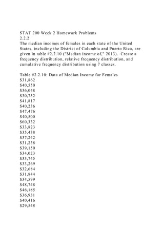
- 1. STAT 200 Week 2 Homework Problems 2.2.2 The median incomes of females in each state of the United States, including the District of Columbia and Puerto Rico, are given in table #2.2.10 ("Median income of," 2013). Create a frequency distribution, relative frequency distribution, and cumulative frequency distribution using 7 classes. Table #2.2.10: Data of Median Income for Females $31,862 $40,550 $36,048 $30,752 $41,817 $40,236 $47,476 $40,500 $60,332 $33,823 $35,438 $37,242 $31,238 $39,150 $34,023 $33,745 $33,269 $32,684 $31,844 $34,599 $48,748 $46,185 $36,931 $40,416 $29,548
- 2. $33,865 $31,067 $33,424 $35,484 $41,021 $47,155 $32,316 $42,113 $33,459 $32,462 $35,746 $31,274 $36,027 $37,089 $22,117 $41,412 $31,330 $31,329 $33,184 $35,301 $32,843 $38,177 $40,969 $40,993 $29,688 $35,890 $34,381 2.2.6 Create a histogram and relative frequency histogram for the data in table #2.2.10. Describe the shape and any findings you can from the graph.
- 3. 2.2.10 Create an ogive for the data in table #2.2.10. Describe any findings you can from the graph. 2.3.4 Table #2.3.7 contains the value of the house and the amount of rental income in a year that the house brings in ("Capital and rental," 2013). Create a scatter plot and state if there is a relationship between the value of the house and the annual rental income. Table #2.3.7: Data of House Value versus Rental Value Rental Value Rental Value Rental Value Rental 81000 6656 77000 4576 75000 7280 67500 6864 95000 7904 94000 8736 90000 6240 85000 7072 121000 12064
- 6. 310000 12480 303000 12272 300000 12480 2.3.8 The economic crisis of 2008 affected many countries, though some more than others. Some people in Australia have claimed that Australia wasn’t hurt that badly from the crisis. The bank assets (in billions of Australia dollars (AUD)) of the Reserve Bank of Australia (RBA) for the time period of March 2007 through March 2013 are contained in table #2.3.11 ("B1 assets of," 2013). Create a time-series plot and interpret any findings. Table #2.3.11: Data of Date versus RBA Assets Date Assets in billions of AUD Mar-2006 96.9 Jun-2006 107.4 Sep-2006 107.2 Dec-2006 116.2 Mar-2007 123.7 Jun-2007 134.0 Sep-2007 123.0 Dec-2007 93.2 Mar-2008 93.7
- 8. Dec-2012 95.8 Mar-2013 90.5 3.1.2 The lengths (in kilometers) of rivers on the South Island of New Zealand that flow to the Pacific Ocean are listed in table #3.1.8 (Lee, 1994). Find the mean, median, and mode. Table #3.1.8: Lengths of Rivers (km) Flowing to Pacific Ocean River Length (km) River Length (km) Clarence 209 Clutha 322 Conway 48 Taieri 288 Waiau 169 Shag 72 Hurunui 138 Kakanui 64 Waipara 64 Rangitata 121
- 9. Ashley 97 Ophi 80 Waimakariri 161 Pareora 56 Selwyn 95 Waihao 64 Rakaia 145 Waitaki 209 Ashburton 90 3.1.8 State which type of measurement scale each represents, and then which center measures can be use for the variable? a.) You collect data on the height of plants using a new fertilizer. b.) You collect data on the cars that people drive in Campbelltown, Australia. c.) You collect data on the temperature at different locations in Antarctica. d.) You collect data on the first, second, and third winner in a beer competition. 3.1.12 An employee at Coconino Community College (CCC) is
- 10. evaluated based on goal setting and accomplishments toward goals, job effectiveness, competencies, CCC core values. Suppose for a specific employee, goal 1 has a weight of 20%, goal 2 has a weight of 20%, goal 3 has a weight of 10%, job effectiveness has a weight of 25%, competency 1 has a goal of 4%, competency 2 has a goal has a weight of 3%, competency 3 has a weight of 3%, competency 4 has a weight of 5%, and core values has a weight of 10%. Suppose the employee has scores of 2.0 for goal 1, 2.0 for goal 2, 4.0 for goal 3, 3.0 for job effectiveness, 2.0 for competency 1, 3.0 for competency 2, 2.0 for competency 3, 3.0 for competency 4, and 4.0 for core values. Find the weighted average score for this employee. If an employee that has a score less than 2.5, they must have a Performance Enhancement Plan written. Does this employee need a plan? 3.2.2 The lengths (in kilometers) of rivers on the South Island of New Zealand that flow to the Pacific Ocean are listed in table #3.2.9 (Lee, 1994). Table #3.2.9: Lengths of Rivers (km) Flowing to Pacific Ocean River Length (km) River Length (km) Clarence 209 Clutha 322 Conway 48 Taieri 288 Waiau 169 Shag
- 11. 72 Hurunui 138 Kakanui 64 Waipara 64 Waitaki 209 Ashley 97 Waihao 64 Waimakariri 161 Pareora 56 Selwyn 95 Rangitata 121 Rakaia 145 Ophi 80 Ashburton 90 a.) Find the mean and median. b.) Find the range. c.) Find the variance and standard deviation. 3.2.6 Print-O-Matic printing company spends specific amounts on fixed costs every month. The costs of those fixed costs are in
- 12. table #3.2.13. Table #3.2.13: Fixed Costs for Print-O-Matic Printing Company Monthly charges Monthly cost ($) Bank charges 482 Cleaning 2208 Computer expensive 2471 Lease payments 2656 Postage 2117 Uniforms 2600 a.) Find the mean and median. b.) Find the range. c.) Find the variance and standard deviation. STAT200 Introduction to Statistics Project 1 STAT200 Introduction to Statistics Project 1 worksheet Objectives: To collect quantitative data, choose appropriate graphs for the data, and then interpret the data. Find the mean, median, mode, and standard deviation of your data. Introduction: This is a very open ended assignment in which you will have to use critical thinking and the knowledge from week 2 to study a population using quantitative variables. It will be important to understand what you population is and what your sample is. Your sample must be appropriate for your population. You will organize your data into appropriate graphs covered in chapter 2, then describe what the graphs tell you about the data.
- 13. Procedure: Start off by asking yourself what you would like to learn about a population. See the work sheet below. You can either collect your own data, use one of the data sets provided in LEO, or find an appropriate data set on the internet. There are data sets available in LEO under “Content Data Sets for Projects”. You should collect/find data that is appropriate for a Histogram, pie chart, stem and leaf diagram, scatter plot, or time series. You should try several of the graphs. For example, for a histogram you could how many hours’ people exercised a week. For a time series you could look at a baseball player’s year by year batting average. Once you have your data, organize the data in an excel spread sheet, then make the appropriate graphs. Be sure to label the axes and add a chart title. For a histogram think about if it should use the frequency or relative frequency. Once you are happy with your charts, copy and paste them into your assignment worksheet and answer the questions. Also copy and paste your data onto the work sheet. Save the document as Lastname_Project2 and turn it in through the assignments folder in LEO. Part 1: Histogram 1. What is your population? 2. What question will you be trying to answer about the population? 3. What is individual? 4. What is your variable? 5. What is your sample? 5. Why is this sample appropriate for your population?
- 14. 6. Insert your data and bar or pie chart below this line. 7. What conclusions can you draw from you chart? Part 2: Time series or scatter plot 1. What is your population? 2. What question will you be trying to answer about the population? 3. What is individual? 4. What are your variables? 5. What is your sample? 5. Why is this sample appropriate for your population? 6. Insert your data and bar or pie chart below this line. 7. What conclusions can you draw from you chart?