SlideShare a Scribd company logo
1 of 63
So, midget bipolars synapse with midget (b) ganglion cells and diffuse 
bipolars synapse with parasol (a) ganglion cells…..
Ganglion Cell Projections to the 
LGN 
• It was already shown that the receptive fields 
of parasol ganglion cells are considerable 
larger than that of midget ganglion cells at the 
same retinal eccentricity.
• It is argued that the smaller receptive fields of 
the midget cells provide greater spatial 
resolution than the parasol cells, which 
integrate energy across a wider range of 
photoreceptors (via horizontal, bipolar, and 
amacrine cells). 
– On the other hand, the sensitivity of the parasol 
cells would be superior. 
• They also differ in their temporal responses. 
– Midget (parvo) cells responding with sustained 
spike trains as long as a light source is projected 
onto the excitatory portions of its receptive fields. 
– Parasol (magno) cells respond at the onset, but 
firing rate quickly goes down the spontaneous rate 
(transient firing).
• The projection of visual space onto 
the retina is such that information 
about objects in the left visual field 
is projected to the right 
hemisphere and information from 
the right field is projected to the left 
hemisphere. 
• The nasal portions of the retina 
cross, while the temporal portions 
project ipsilaterally. 
• In evolution, the decussating 
(crossing) path is the oldest. 
– As the eyes moved medially, the 
ipsilateral pathway developed. 
– This results in greater visual field 
overlap (C-D), and the ipsilateral 
pathway assures that the inputs 
from the overlapping fields go to 
both cortices. 
Input (letters A-F) from the right visual field are mapped in an orderly fashion 
to the left LGN, while the left visual field projects to the right LGN. 
The top 4 layers form the parvocellular layers and receive input from midget 
ganglion cells. 
The bottom 2 layers from the magnocellular layers and receive input from 
parasol ganglion cells.
• If one measures the conduction 
times for electrical signals traveling 
from the retina to the parvocellular 
layers of the LGN, they are longer 
than the latencies to the 
magnocellular layer (on the 
average). 
o Schiller and Malpeli (1978) 
applied an electrical stimulus at 
the optic chiasm and measured 
the time it took the signal to 
travel to the various layers. 
• The receptive fields of LGN cells 
are not appreciably different from 
those of ganglion cells, but LGN 
cells are influenced by descending 
input from the cortex (visual and 
other areas), the brainstem, from 
other cells in the thalamus, from 
other LGN cells 
• The descending input from cortex 
to the LGN is actually more 
substantial the that projections from 
the LGN to the cortex!
• The fact that the LGN contains a 
retinotopic map can be seen in 
oblique, electrode tracks. 
• This is significant because it 
demonstrates that neurons entering 
the LGN are arranged so that fibers 
carrying signals from the same area 
of the retina end up the same area of 
the LGN, and neighboring retinal 
regions project to neighboring LGN 
regions. 
• Retinotopic maps occur in each of 
the layers, and the maps line up 
with each other, as seen in 
perpendicular electrode penetrations 
(all neurons would have receptive 
fields at the same locations). 
B A 
CC’ B’A’ 
C
• The corpus callosum, which consists of fiber 
tracts between the two hemispheres, 
integrates the left and right visual fields so 
well that we do not notice that they are 
encoded independently. 
• The geniculostriate pathway (LGN to cortex) 
is clearly the most important and most 
recently evolved. 
• About 90% of the optic nerve fibers go to 
the lateral geniculate body. 
• The other 10% go to the superior colliculus, 
consisting of collaterals from the 
geniculostriate pathway and possibly a few 
direct fibers projecting from the optic nerves. 
• In non-mammalian species (e.g., birds and 
fish) superior colliculus is called the optic 
tectum, and it serves the function of the 
geniculostriate pathway (color, form).
• For mammals, the superior colliculus 
appears to play a role in the 
orientation of the animal in space. 
• Snyder found that lesions of the 
superior colliculi of hamsters 
produced behavior that is consistent 
with deficits in orientation but not 
discrimination. 
• Animals forced to discriminate 
horizontal from vertical bars do 
horribly if they must run down a left 
or right alley, but perform well in 
go/no go tasks. 
o It is as though they can discriminate 
vertical from horizontal but cannot 
tell left from right (they do not get 
reinforcement because they bump 
into objects along the way). 
o Note the importance of the task 
performed by the animal, because 
many early researchers concluded 
that lesions of the superior colliculi 
produced blindness while others 
claimed no effect of the lesions.
Striate Cortex 
• The very rear of the occipital lobe is 
where the LGN projects. 
• The area has several different 
names: primary visual cortex, V1, 
area 17, or striate cortex (because 
of the striped pattern it takes on 
after staining). 
• It consists of 6 major layers, some 
having sublayers. 
Fibers from the LGN project mainly 
into layer 4, with magnocellular 
neurons (2 ventral LGN layers) 
coming into layer 4Cα and 
parvocellular neurons (4 dorsal 
layers) coming into layer 4Cβ. 
α 
b
Recording From Units in V1
Recording From Units in V1 
• The first recordings in Area 17 were made by 
Jung in Germany in the mid 1950's from cats. 
– At the time, little was known about the responses 
of the earlier cells in the pathway, and the study 
was a dismal failure. 
– Jung presented flashes of light and concluded that 
90 95% of the cells in the visual ‑ cortex simply did 
not respond to light. 
– This was most likely due to the size of his flashes, 
which produced a balance of inhibition and 
excitation from the center‑surround fields.
Recording From Units in V1 
• All that changed in the late 1950’s with 
the pioneering work of David Hubel and 
Torsten Wiesel.
David Hubel
Torsten Wiesel
Recording From Units in V1 
• David Hubel and Torsten Wiesel knew what types of information 
were passed along from lower levels of the system, since 
Torsten Wiesel had worked in Stephen Kuffler’s lab at Johns 
Hopkins in 1955. 
– Kuffler had carried out measurements of receptive fields of cat 
ganglion cells, and this knowledge of center-surround antagonism 
meant that Hubel and Wiesel stood a much better chance of asking 
intelligent questions of the cortex. 
– Because they knew of surround inhibition, they used patterned 
stimuli that could maximize the probability of evoking responses. 
– Their major contribution was that they found cells whose receptive 
fields were elongated, orientationally specific, and more spatially 
selective than LGN cells. 
– Even with this knowledge, they still had difficulty getting cells to 
respond to light. 
• As they gained a better understanding of what sorts of 
information were being processed, a greater percentage of cells 
could be driven. 
– In 1959 they claimed that 50% could be driven, but by 1962 the 
percentage was around 90 (once they found the length specificity). 
• They were awarded the Nobel Prize in Physiology or Medicine 
in 1981.
• "Simple" cells were the first from which recordings were 
made, with receptive fields consisting of discrete 
inhibitory and excitatory regions. 
• Some of these have bipartite fields and others have 
tripartite fields. 
• They had clearly defined excitatory and inhibitory 
regions. 
• About 80% of the simple cells are binocular, having 
similar receptive fields for the two eyes.
• The elongation makes these cells orientation specific, with 
the preferred orientation varies from cell to cell. 
• One idea was to take the outputs of LGN cells an align 
them in such a way to produce various elongated 
receptive fields.
Complex Cells 
1 2 3 4 5 
• "Complex" cells do not have discrete excitatory and inhibitory 
subregions. 
– If their receptive fields are mapped with small spots of light, one 
finds a mixture of small areas of excitation and inhibition, with only 
very small responses. 
– The optimal stimulus is a light or dark bar somewhere in the field 
that must not cover too large of a region. 
– Complex cells respond to the bar in any one of the subregions, but 
the response diminishes as the bar covers more that one region at 
a time; they all prefer moving bars. 
– About 25% are directionally selective, preferring a moving stimulus 
in one direction across the field (15 vs. 51). 
– Like simple cells, complex cells are orientationally selective. 
– As it turns out, approximately 75% of cortical neurons are classified 
as complex. 
• As such, it is hardly surprising that researchers had difficulty getting 
them to respond to light, since most used stationary stimuli.
Hypercomplex" cells are like simple or complex cells, except that they are 
end stopped on one or both sides to produce ‑ length specificity. 
They are now thought to reflect subclasses of simple and complex cells. 
Simple cells
Hierarchical Model 
• Hubel and Wiesel believed that the 
outputs of center-surround ganglion cells 
projected to the LGN (remaining center-surround), 
with multiple cells from the LGN 
then projecting onto a single cortical 
neuron. 
• Multiple simple cell outputs could then 
project onto a 2nd level cortical neuron, 
producing complex cell receptive fields.
Simple Cells 
LGN cells 
Simple Cell 
Retina
Complex Cells 
- 
- 
- 
- 
- 
- 
- 
- 
- 
- 
- 
- 
- 
- 
- 
- 
- 
- 
- 
- 
- 
- 
- 
- 
- 
- 
+ 
+ 
+ 
+ 
+ 
- 
- 
+ 
+ 
+ 
+ 
+ 
- 
- 
+ 
+ 
+ 
+ 
+ 
- 
- 
- 
- 
- 
- 
- 
- 
- 
- 
+ 
+ 
+ 
+ 
+ 
Simple Cells 
Retina Complex Cell
A Video Showing the Difference 
between Simple and Complex Cells 
www.youtube.com/watch?v=8VdFf3egwfg
The Hubel and Wiesel View of 
Spatial Vision 
• Because they demonstrated receptive fields that 
were either bipartite (edge detectors) or tripartite 
(line or bar detectors), their findings were 
consistent with an atomistic approach. 
– The argued that the fundamental building blocks of 
objects were lines and edges at particular positions, 
orientations, widths, lengths, contrasts, etc. 
– Higher level shapes could be constructed by 
assembling the receptive fields of simple, complex, 
and hypercomplex cells found in V1.
Source of Inhibition? 
• Note that all of the inhibition in the hierarchical model is 
generated within the retina. 
• Creutzfeld and his colleagues (1974) recorded 
intracellularly from cortical cells (a monumental task) 
while stimulating units in the LGN. 
– In all cases the LGN input was excitatory, and the inhibition 
observed had a longer latency (probably stemming from 
cortical interactions). 
• Sillito (1975, 1980) performed experiments in which 
GABA antagonists (bicuculine) was applied 
iontophoretically to the cortex in the vicinity of a 
recording site. 
– It eliminated both orientation and direction of movement 
tuning, implying that they arise from interactions within cortex. 
• Another criticism of the hierarchical model is the fact 
that it is quite difficult to imagine how the response 
properties of complex cells can be generated by 
recombining simple cell outputs.
“A” Detector 
- 
- 
- 
- 
- 
+ 
+ 
+ 
+ 
+ 
- 
- 
----- 
- 
- 
- 
- 
- 
- 
- 
- 
- 
+++++ 
- 
- 
- 
- 
+ 
+ 
+ 
+ 
+ 
----- 
Retina
Striate Architecture 
• Given that cells are “tuned” to different orientations, position, 
sizes, colors, etc., the question arises as to how these features 
are distributed across the cortex. 
– This is a question of the architecture of the striate cortex—what is 
the spatial layout and pattern of interconnections among cells tuned 
to different values of these different stimulus dimensions? 
– Answering this required Herculean recording sessions in which 
researchers would find a cell and record from it until they 
determined the optimal location, orientation, size, and eye 
dominance. 
– The microelectrode would then by moved a but further until another 
cells was isolated. 
• It’s “best features” would then be determined. 
• This process was repeated until a great many cells were examined, 
then the animal would be “sacrificed” and its brain examined 
microscopically to determine the location of the electrode tracts. 
– This endeavor was vastly progressed by the development of 
autoradiographic techniques that rely on the uptake of radioactive 
sugar into highly active cells (2-deoxyglucose studies), which 
generally corroborated the single-unit recording data.
Retinotopic Map 
• The layered sheets of cells that comprise 
primary visual cortex within each hemisphere 
are laid out in a retinotopic map of exactly half 
the visual field. 
• The map preserves retinal topography, with 
nearby points on the retina projecting to nearby 
cortical points. 
• The metric properties of the map on the cortex 
are distorted, however. 
– The main distortion is due to cortical magnification of 
central (foveal) areas relative to peripheral ones.
• Magnification is from the 2-deoxyglucose 
study of Tootell et al. (1982).
• Tootel, Silverman, Switkes, and De Valois 
(1982) • Since glucose is the metabolite of cortical 
neurons, more is used by active cells. 
• 2-deoxyglucose (2DG) is taken up by cells 
as if it were glucose, but it remains in cells 
(isn’t actually metabolized). 
• Since it is radioactive, one determines 
where it accumulates when a particular 
stimulus is presented. 
• A “rings and rays” pattern (A) centered on 
the fovea was presented while the monkey 
was injected with 2DG. 
o The rings and rays display was 
composed of small (randomly sized) 
rectangles that flickered over time, 
with the rings spaced logarithmically 
(from the center).
• Tootel, Silverman, Switkes, and De Valois 
(1982) •The cortical surface is flattened, then sliced 
thinly parallel to the surface and placed on 
X-ray sensitive film. 
•The logarithmically spaced rings stimulate 
strips in V1 that are about equally spaced 
on the cortex, indicting that a small region 
near the fovea activates a 
disproportionately large area of cortex. 
o Peripheral regions stimulate smaller 
Foveal cortical regions. 
On left Activation caused by hemicircles. 
Activation caused by radii.
Ocular Dominance Slabs 
• We have two eyes, and both project to both 
hemispheres. 
• This raises the question as to whether we have 
separate retinotopic maps in the cortex or one 
integrated one. 
– The answer lies somewhere in between—there is one 
global map for each cortex, within which cells that are 
dominated by one eye or the other are interleaved. 
– Ocular dominance varies from one eye being 
dominant to both eyes being equally effective at 
driving a cell.
In population studies of ocular dominance, Hubel and Wiesel studied 
hundreds of cells and categorized each one as belonging to one of seven 
arbitrary groups. A group 1 cell was defined as a cell influenced only by 
the contralateral eye—the eye opposite to the hemisphere in which it sits. 
A group 2 cell responds to both eyes but strongly prefers the 
contralateral eye. And so on. 
Clearly there are differences between cat and macaque….. Rhesus macaques show few 
cells that are driven equally well by the two eyes while they are quite prevalent in cats.
Light is right Stimulus was a vertical line; eye, dark is left eye 
spacing is about every 0.5 mm. 
The figure at the left is an optical image 
of superimposed orientation columns. 
Again it is found that the full range of 
orientations is represented every 0.5 
mm.
The Hypercolumn 
• These findings lead us to the concept of 
the hypercolumn. 
– Overall, V1 is composed of many smaller 
cortical modules called hypercolumns. 
– They are long and then running perpendicular 
to the cortical surface through all 6 layers. 
– Every 1 mm2 represents a full range of 
orientations for right and left eye dominance.
Shown here are two adjacent 
hyperocolumns, representing 
adjacent point on the retina. 
Every square mm represented 
both occular dominances, with 
orientations between 0 and 180o 
represented twice 
http://www.sinauer.com/wolfe2e/chap3/hypercolumnsF.htm
The interspersed “blobs” 
represent wavelength 
processing.
Two adjacent hypercolumns are 
represented in a 2 x 2 mm slab of 6 cortical 
layers.
Adaptation 
• The rationale of psychophysical adaptation 
studies is that long term exposure to a given 
stimulus fatigues channels responsive to it, 
so that later perception is based on an altered 
distribution of activity across channels tuned 
to some dimension. 
• This shift results in a change in the percept 
experienced in the unadapted state. 
• This allows psychophysical studies to 
elucidate the presence of tuned channels. 
• The following slides use orientation tuning as 
an example….
• Let your gaze move back and forth over 
the fixation dash, adapting the upper 
half of your visual field to a tilt of -20o 
and the lower half to +20o.
Example
• Most subjects report that the vertical 
lines in the upper half appear to be 
tilted to the right, while the lower vertical 
lines appear to be tilted to the left. 
• What’s going on here?
In the unadapted state, Orientation X causes equal activity of channel 
A and B. Say you adapt to Orientation W, reducing the 
responsiveness of the A orientation channel. Orientation X would now 
be perceived to have a greater orientation, since it is causing greater 
activation of Channel B than Channel A. 
A B 
Orientation 
Response 
X 
W
On the other hand, say you adapt to Orientation Y, reducing the 
responsiveness of the B orientation channel. Orientation X would now 
be perceived to have a smaller degree of tilt, since it is causing 
greater activation of Channel A than Channel B. 
A B 
Orientation 
Response 
X 
Y
Spatial Frequency Analysis 
• No one doubts the contributions made by 
Hubel and Wiesel, and the enormous leap 
forward the visual science made on account 
of their ability to “drive” visual cortical 
neurons. 
– At issue is the question of whether or not cells 
truly prefer bars of different widths. 
• I introduced the idea of a spatial modulation 
transfer function as a measure of the ability of 
humans to resolve spatial frequency. 
– Threshold contrast was measured as a function of 
the spatial frequency of sinusoidal gratings, 
yielding functions like this:
• The spatial MTF shows best sensitivity to a 
mid range of spatial frequencies (5-7 cycles 
per degree), with sensitivity to higher and 
lower spatial frequencies being somewhat 
lower.
• This can be easily 
explained on the 
basis of center-surround 
receptive 
fields found at the 
bipolar cell, 
ganglion cell, and 
LGN levels. 
• Low spatial 
frequencies excite 
both center and 
surround uniformly, 
as do high spatial 
frequencies. 
• Intermediate spatial 
frequencies excite 
the center but not 
the surround (or 
vice versa).
• It was Campbell and Robson (1969) who had the audacity to 
propose that the overall spatial MTF was based on the 
“envelope” of tuned spatial frequency channels, shown in the 
right panel. 
– Essentially the visual system would consist of multiple spatial 
frequency-tuned channels, and we would know the form of the 
stimulus by knowing what spatial frequencies were present. 
• At the heart of spatial frequency theory is the notion that all 
complex distributions of luminance fluctuations across space 
can be recreated by adding spatial sinusoids of known spatial 
frequency, amplitude (contrast), orientation, and phase. 
• It seems strange to consider spatial frequencies as the 
“primitives” or atoms of visual perception because we do not 
consciously experience their presence with analyzing complex 
scenes.
• Odd integer harmonics are added 
together at an amplitude that is harmonic 
number….
• The idea is that we would perceive a 
square wave because spatial frequency 
tuned channels at f, 3f, 5f, 7f, etc would 
be active, each less active that the one 
preceding it since there is less power in 
higher harmonics.
Back to Campbell and 
Robson… 
• If one adapts to a 7 c/deg grating, sensitivity is only lost near 7 c/deg. 
• Sensitivity is only lost near the adapting spatial frequency, as though 
the channel were fatigued by the adapting stimulus. 
• The middle panel shows the difference between the unadapted and 
adapted MTF, and can be thought of as inferring the shape of a spatial 
frequency channel. 
• But does it mean that spatial frequency per se is the variable encoded 
by the visual system rather than bar width? 
– Unfortunately, the visual system could be encoding the sinusoidal grading 
as a blurry bar of a particular width, so one could interpret these findings as 
demonstrating the loss of sensitivity to bars of particular widths.
• So what if one adapted to a square 
wave? 
– If the visual system were tuned to bar 
widths, then this adapting stimulus should 
cause reductions in sensitivity at the spatial 
frequency corresponding to the bar width, 
but not at other spatial frequencies. 
– If, on the other hand, the extracted 
dimension were spatial frequency per se, 
then sensitivity should be lost at the odd 
harmonics.
3 9 
Spatial Freq. (c/deg) 
• There is loss at the fundamental (3 c/deg) and the 3rd harmonic 
(9 c/deg)! 
– Unless the fundamental frequency is very low, there is no real 
opportunity to observe the loss in sensitivity at the 3F because (a) 
sensitivity falls off so abruptly with spatial frequency and (b) there is 
likely inhibition between adjacent spatial frequency channels. 
• The inhibition between channels means that 1F and 3F and 3F and 5F 
are likely to reduce the effectiveness of each other. 
• Since the power in the stimulus goes down by the harmonic number, 1F 
will squash the activation level of 3F and 3F with squash the activation 
level of 5F IN THE VISUAL SYSTEM!
• Graham and Nachmias (1971) 
found that the threshold for 
detecting a compound of f+3f 
could be predicted from the 
magnitudes of the individual 
components regardless of whether 
they are added in “peaks add” or 
“peaks subtract” phase. 
• If the system computed the 
contrast of the pattern, sensitivity 
to “peaks add” stimuli would have 
been much better than to the 
“peaks subtract” stimuli because 
of the manner in which contrast is 
computed. 
• Graham and Nachmias (1971) 
found that the threshold for 
detecting a compound of f+3f 
could be predicted from the 
magnitudes of the individual 
components regardless of 
whether they are added in 
“peaks add” or “peaks subtract” 
phase. 
• If the system computed the 
contrast of the pattern, sensitivity 
to “peaks add” stimuli would 
have been much better than to 
the “peaks subtract” stimuli 
because of the manner in which 
contrast is computed. 
C o n t r a s t 
L L 
L L 
= 
- 
+ 
m a x m i n 
m a x m i n
Adapt to the following gratings, ala 
Blakemore and Sutton (1969)
In the un-adapted state, Spatial Frequency X causes equal activity of 
channel A and B. causes equal activation of the short and long 
channels. Say you adapt to Spatial Frequency W, reducing the 
responsiveness of the B channel. Spatial Frequency X would now be 
perceived to have a lower spatial frequency, since it is causing 
greater activation of Channel A than Channel B (adapting to a higher 
spatial frequency shifts the appearance to lower spatial frequencies). 
A B C 
Spatial Frequency 
Response 
X 
W
Adapting to lower spatial frequencies makes higher spatial 
frequencies look even higher, since the C channel is now much more 
active than channel B. 
A B C 
Spatial Frequency 
Response 
X 
W
Cortical Recordings 
• Recordings from cortical cells are often interpreted now in terms of the range 
of spatial frequencies to which the cells respond rather than in terms of the 
bar widths to which they are sensitive. 
• If gratings are used, cortical cells seem to be rather narrowly tuned, with 
bandwidths of about 1.5 octaves (log base 2 of bandwidth) at points at which 
sensitivity has fallen by a factor of 2 (relative to the peak). 
– This means that the ratio of the higher to lower spatial frequencies at the half-sensitivity 
points is 21.5 or 2.8 on the average. 
• The distribution of bandwidths is quite large, with the monkey's foveal cortex 
containing as many cell with bandwidths of 2.5 octaves as there are cells 
with bandwidths of 0.7 octaves. 
– In general, about a third of the cortical cells have bandwidths between 0.5 and 1.2 
octaves, while a small sample are tuned like LGN cells. 
– By comparison, the bandwidths of cells in the LGN (X-cells) are 3-4 octaves in the 
cat and may exceed 5 octaves in the monkey, so the narrower cortical bandwidths 
must be due to intracortical interactions. 
• In general cortical cells have bandwidths that increase logarithmically with 
peak spatial frequency, so the "octave" measure of tuning stays roughly 
constant with peak spatial frequency (it declines slightly with increasing peak 
spatial frequency). 
• Differences in peak frequency are slight for simple and complex cells-- 
complex cells tend to be tuned to slightly higher spatial frequencies. 
• Larger receptive fields (and low peak SFs) are generally found to emanate 
from parafoveal regions, and there are fewer high-spatial frequency tuned 
cells in extrafoveal cortical regions.
It is critical for the theory that any point in space be analyzed by elements 
tuned to different spatial frequencies, so the previous statement reflects 
general trends when one measures best spatial frequency as a function of 
retinal eccentricity.
Local Spatial Frequency 
Analysis 
Since receptive fields of cortical neurons 
is restricted, we believe that the system 
carries out a local spatial frequency 
analysis (no cell “sees” the entire visual 
field). 
The elements are modeled as Gabor 
functions (Gaussian multiplied sine 
waves).
• The figure below shows the relative contributions of 
high and low spatial frequency information. 
– (a) shows a complete face, (b) presents the same face 
with only high spatial frequency components and (c) 
shows the same face with only low spatial frequency 
components. 
– Low frequencies convey information about general shape 
and form, while high frequency information provides the 
detail.

More Related Content

What's hot

Myopia classification and management by Tahir Shaukat
Myopia classification and management by Tahir Shaukat Myopia classification and management by Tahir Shaukat
Myopia classification and management by Tahir Shaukat Optometry Club
 
Physiology of Retina
Physiology of RetinaPhysiology of Retina
Physiology of RetinaNajara Thapa
 
Interpretation of OCT(Glaucoma)
Interpretation of OCT(Glaucoma)Interpretation of OCT(Glaucoma)
Interpretation of OCT(Glaucoma)Shylesh Dabke
 
ANATOMY OF CHOROID.pptx
ANATOMY OF CHOROID.pptxANATOMY OF CHOROID.pptx
ANATOMY OF CHOROID.pptxudayasree30
 
Anatomy and embryology of crystalline lens DrBP
Anatomy and embryology of crystalline lens DrBPAnatomy and embryology of crystalline lens DrBP
Anatomy and embryology of crystalline lens DrBPdrbhushan17
 
Visible light and the retina
Visible light and the retinaVisible light and the retina
Visible light and the retinaYasuo Yanagi
 
Diabetic retinopathy
Diabetic retinopathyDiabetic retinopathy
Diabetic retinopathyRiyad Banayot
 
IOL implantation in the absence of capsular bag
IOL implantation in the absence of capsular bagIOL implantation in the absence of capsular bag
IOL implantation in the absence of capsular bagcrisnemato
 
Ophthalmology Problems
Ophthalmology ProblemsOphthalmology Problems
Ophthalmology ProblemsDrAfiqahMF
 
Orbital Inflammations.pptx
Orbital Inflammations.pptxOrbital Inflammations.pptx
Orbital Inflammations.pptxdratulkranand
 
Corneal physiology ‫‬
Corneal physiology ‫‬Corneal physiology ‫‬
Corneal physiology ‫‬Opto Ihsan MH
 
Anatomy of Retina
Anatomy of RetinaAnatomy of Retina
Anatomy of RetinaSai Sandeep
 
Physiology of lens and Cataractogenesis
Physiology of lens and CataractogenesisPhysiology of lens and Cataractogenesis
Physiology of lens and CataractogenesisSristiThakur
 

What's hot (20)

Optic Neuritis.pptx
Optic Neuritis.pptxOptic Neuritis.pptx
Optic Neuritis.pptx
 
Cmv retinitis
Cmv retinitisCmv retinitis
Cmv retinitis
 
Myopia classification and management by Tahir Shaukat
Myopia classification and management by Tahir Shaukat Myopia classification and management by Tahir Shaukat
Myopia classification and management by Tahir Shaukat
 
Abnormal reactions of pupil
Abnormal reactions of pupilAbnormal reactions of pupil
Abnormal reactions of pupil
 
Physiology of Retina
Physiology of RetinaPhysiology of Retina
Physiology of Retina
 
Interpretation of OCT(Glaucoma)
Interpretation of OCT(Glaucoma)Interpretation of OCT(Glaucoma)
Interpretation of OCT(Glaucoma)
 
ANATOMY OF CHOROID.pptx
ANATOMY OF CHOROID.pptxANATOMY OF CHOROID.pptx
ANATOMY OF CHOROID.pptx
 
Anatomy and embryology of crystalline lens DrBP
Anatomy and embryology of crystalline lens DrBPAnatomy and embryology of crystalline lens DrBP
Anatomy and embryology of crystalline lens DrBP
 
Visible light and the retina
Visible light and the retinaVisible light and the retina
Visible light and the retina
 
Genetics in Ophthalmology
Genetics in OphthalmologyGenetics in Ophthalmology
Genetics in Ophthalmology
 
Embryology of Eye
Embryology of EyeEmbryology of Eye
Embryology of Eye
 
Diabetic retinopathy
Diabetic retinopathyDiabetic retinopathy
Diabetic retinopathy
 
IOL implantation in the absence of capsular bag
IOL implantation in the absence of capsular bagIOL implantation in the absence of capsular bag
IOL implantation in the absence of capsular bag
 
Ophthalmology Problems
Ophthalmology ProblemsOphthalmology Problems
Ophthalmology Problems
 
Orbital Inflammations.pptx
Orbital Inflammations.pptxOrbital Inflammations.pptx
Orbital Inflammations.pptx
 
Corneal physiology ‫‬
Corneal physiology ‫‬Corneal physiology ‫‬
Corneal physiology ‫‬
 
Anatomy of Retina
Anatomy of RetinaAnatomy of Retina
Anatomy of Retina
 
CRVO
CRVOCRVO
CRVO
 
Physiology of lens and Cataractogenesis
Physiology of lens and CataractogenesisPhysiology of lens and Cataractogenesis
Physiology of lens and Cataractogenesis
 
Intraocular lens
Intraocular lensIntraocular lens
Intraocular lens
 

Viewers also liked

Machine Learning and Data Mining: 10 Introduction to Classification
Machine Learning and Data Mining: 10 Introduction to ClassificationMachine Learning and Data Mining: 10 Introduction to Classification
Machine Learning and Data Mining: 10 Introduction to ClassificationPier Luca Lanzi
 
SPM 12 practical course by Volodymyr B. Bogdanov (Kyiv 2015, Day 2)
SPM 12 practical course by Volodymyr B. Bogdanov (Kyiv 2015, Day 2) SPM 12 practical course by Volodymyr B. Bogdanov (Kyiv 2015, Day 2)
SPM 12 practical course by Volodymyr B. Bogdanov (Kyiv 2015, Day 2) Volodymyr Bogdanov
 
Mod 14 Basic Concepts and Vision
Mod 14   Basic Concepts and VisionMod 14   Basic Concepts and Vision
Mod 14 Basic Concepts and VisionTina Medley
 
PSY 150 403 CHAPTER 6 SLIDES
PSY 150 403 CHAPTER 6 SLIDESPSY 150 403 CHAPTER 6 SLIDES
PSY 150 403 CHAPTER 6 SLIDESkimappel
 
Deep Learning - Convolutional Neural Networks
Deep Learning - Convolutional Neural NetworksDeep Learning - Convolutional Neural Networks
Deep Learning - Convolutional Neural NetworksChristian Perone
 
3 Things Every Sales Team Needs to Be Thinking About in 2017
3 Things Every Sales Team Needs to Be Thinking About in 20173 Things Every Sales Team Needs to Be Thinking About in 2017
3 Things Every Sales Team Needs to Be Thinking About in 2017Drift
 
How to Become a Thought Leader in Your Niche
How to Become a Thought Leader in Your NicheHow to Become a Thought Leader in Your Niche
How to Become a Thought Leader in Your NicheLeslie Samuel
 

Viewers also liked (9)

Machine Learning and Data Mining: 10 Introduction to Classification
Machine Learning and Data Mining: 10 Introduction to ClassificationMachine Learning and Data Mining: 10 Introduction to Classification
Machine Learning and Data Mining: 10 Introduction to Classification
 
SPM 12 practical course by Volodymyr B. Bogdanov (Kyiv 2015, Day 2)
SPM 12 practical course by Volodymyr B. Bogdanov (Kyiv 2015, Day 2) SPM 12 practical course by Volodymyr B. Bogdanov (Kyiv 2015, Day 2)
SPM 12 practical course by Volodymyr B. Bogdanov (Kyiv 2015, Day 2)
 
Mod 14 Basic Concepts and Vision
Mod 14   Basic Concepts and VisionMod 14   Basic Concepts and Vision
Mod 14 Basic Concepts and Vision
 
PSY 150 403 CHAPTER 6 SLIDES
PSY 150 403 CHAPTER 6 SLIDESPSY 150 403 CHAPTER 6 SLIDES
PSY 150 403 CHAPTER 6 SLIDES
 
Visual pathway
Visual pathwayVisual pathway
Visual pathway
 
Deep Learning - Convolutional Neural Networks
Deep Learning - Convolutional Neural NetworksDeep Learning - Convolutional Neural Networks
Deep Learning - Convolutional Neural Networks
 
SlideShare 101
SlideShare 101SlideShare 101
SlideShare 101
 
3 Things Every Sales Team Needs to Be Thinking About in 2017
3 Things Every Sales Team Needs to Be Thinking About in 20173 Things Every Sales Team Needs to Be Thinking About in 2017
3 Things Every Sales Team Needs to Be Thinking About in 2017
 
How to Become a Thought Leader in Your Niche
How to Become a Thought Leader in Your NicheHow to Become a Thought Leader in Your Niche
How to Become a Thought Leader in Your Niche
 

Similar to Cnshubelandwiesel

physiologyofvision3-20052207035073637.pdf
physiologyofvision3-20052207035073637.pdfphysiologyofvision3-20052207035073637.pdf
physiologyofvision3-20052207035073637.pdfRavi180910
 
PHYSIOLOGY OF VISION
PHYSIOLOGY OF VISIONPHYSIOLOGY OF VISION
PHYSIOLOGY OF VISIONPriyanka Raj
 
08b vision processing form and shape
08b vision processing form and shape08b vision processing form and shape
08b vision processing form and shapePS Deb
 
08b vision processing form and shape
08b vision processing form and shape08b vision processing form and shape
08b vision processing form and shapePS Deb
 
Neurons and the glia.pptx
Neurons and the glia.pptxNeurons and the glia.pptx
Neurons and the glia.pptxSabaJahan2
 
Positioning system in the brain the brain’s navigational place [autosaved]
Positioning system in the brain the brain’s navigational place [autosaved]Positioning system in the brain the brain’s navigational place [autosaved]
Positioning system in the brain the brain’s navigational place [autosaved]adityadayana
 
VISUAL PERCEPTION AND NEUROPHYSIOLOGY
VISUAL PERCEPTION AND NEUROPHYSIOLOGYVISUAL PERCEPTION AND NEUROPHYSIOLOGY
VISUAL PERCEPTION AND NEUROPHYSIOLOGYMarion Kemboi
 
Anatomy of the Human Eye ( PDFDrive ).pdf
Anatomy of the Human Eye ( PDFDrive ).pdfAnatomy of the Human Eye ( PDFDrive ).pdf
Anatomy of the Human Eye ( PDFDrive ).pdfRockyIslam5
 
Visual evoked potentials
Visual evoked potentialsVisual evoked potentials
Visual evoked potentialsDhaval Modi
 
Magnocellular and Parvocellular pathways1.pptx
Magnocellular and Parvocellular pathways1.pptxMagnocellular and Parvocellular pathways1.pptx
Magnocellular and Parvocellular pathways1.pptxLaithLutfi1
 
Dorso-Lateral Geniculate Nucleus and Parallel Processing
Dorso-Lateral Geniculate Nucleus and Parallel ProcessingDorso-Lateral Geniculate Nucleus and Parallel Processing
Dorso-Lateral Geniculate Nucleus and Parallel ProcessingGauriSShrestha
 
COGS 107B - Winter 2010 - Lecture 4 - The visual system I
COGS 107B - Winter 2010 - Lecture 4 -  The visual system I COGS 107B - Winter 2010 - Lecture 4 -  The visual system I
COGS 107B - Winter 2010 - Lecture 4 - The visual system I Tim Mullen
 
Physiology of the visual pathway & cerebral integration
Physiology of the visual pathway & cerebral integrationPhysiology of the visual pathway & cerebral integration
Physiology of the visual pathway & cerebral integrationHenok Samuel
 
The retina (histology and physiology)
The retina (histology and physiology)The retina (histology and physiology)
The retina (histology and physiology)مصطفى حكمت
 

Similar to Cnshubelandwiesel (20)

Visual pathway
Visual pathwayVisual pathway
Visual pathway
 
physiologyofvision3-20052207035073637.pdf
physiologyofvision3-20052207035073637.pdfphysiologyofvision3-20052207035073637.pdf
physiologyofvision3-20052207035073637.pdf
 
PHYSIOLOGY OF VISION
PHYSIOLOGY OF VISIONPHYSIOLOGY OF VISION
PHYSIOLOGY OF VISION
 
08b vision processing form and shape
08b vision processing form and shape08b vision processing form and shape
08b vision processing form and shape
 
08b vision processing form and shape
08b vision processing form and shape08b vision processing form and shape
08b vision processing form and shape
 
Neurons and the glia.pptx
Neurons and the glia.pptxNeurons and the glia.pptx
Neurons and the glia.pptx
 
visualsystem.ppt
visualsystem.pptvisualsystem.ppt
visualsystem.ppt
 
Positioning system in the brain the brain’s navigational place [autosaved]
Positioning system in the brain the brain’s navigational place [autosaved]Positioning system in the brain the brain’s navigational place [autosaved]
Positioning system in the brain the brain’s navigational place [autosaved]
 
PHYSIOLOGY OF RETINA.pptx
PHYSIOLOGY OF RETINA.pptxPHYSIOLOGY OF RETINA.pptx
PHYSIOLOGY OF RETINA.pptx
 
Animal behavior & its relation to coordination systems
Animal behavior & its relation to coordination systemsAnimal behavior & its relation to coordination systems
Animal behavior & its relation to coordination systems
 
Visual pathway
Visual pathwayVisual pathway
Visual pathway
 
VISUAL PERCEPTION AND NEUROPHYSIOLOGY
VISUAL PERCEPTION AND NEUROPHYSIOLOGYVISUAL PERCEPTION AND NEUROPHYSIOLOGY
VISUAL PERCEPTION AND NEUROPHYSIOLOGY
 
Anatomy of the Human Eye ( PDFDrive ).pdf
Anatomy of the Human Eye ( PDFDrive ).pdfAnatomy of the Human Eye ( PDFDrive ).pdf
Anatomy of the Human Eye ( PDFDrive ).pdf
 
Edge detection
Edge detectionEdge detection
Edge detection
 
Visual evoked potentials
Visual evoked potentialsVisual evoked potentials
Visual evoked potentials
 
Magnocellular and Parvocellular pathways1.pptx
Magnocellular and Parvocellular pathways1.pptxMagnocellular and Parvocellular pathways1.pptx
Magnocellular and Parvocellular pathways1.pptx
 
Dorso-Lateral Geniculate Nucleus and Parallel Processing
Dorso-Lateral Geniculate Nucleus and Parallel ProcessingDorso-Lateral Geniculate Nucleus and Parallel Processing
Dorso-Lateral Geniculate Nucleus and Parallel Processing
 
COGS 107B - Winter 2010 - Lecture 4 - The visual system I
COGS 107B - Winter 2010 - Lecture 4 -  The visual system I COGS 107B - Winter 2010 - Lecture 4 -  The visual system I
COGS 107B - Winter 2010 - Lecture 4 - The visual system I
 
Physiology of the visual pathway & cerebral integration
Physiology of the visual pathway & cerebral integrationPhysiology of the visual pathway & cerebral integration
Physiology of the visual pathway & cerebral integration
 
The retina (histology and physiology)
The retina (histology and physiology)The retina (histology and physiology)
The retina (histology and physiology)
 

Cnshubelandwiesel

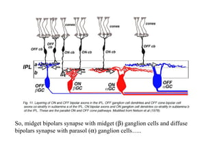
  • 1. So, midget bipolars synapse with midget (b) ganglion cells and diffuse bipolars synapse with parasol (a) ganglion cells…..
  • 2. Ganglion Cell Projections to the LGN • It was already shown that the receptive fields of parasol ganglion cells are considerable larger than that of midget ganglion cells at the same retinal eccentricity.
  • 3. • It is argued that the smaller receptive fields of the midget cells provide greater spatial resolution than the parasol cells, which integrate energy across a wider range of photoreceptors (via horizontal, bipolar, and amacrine cells). – On the other hand, the sensitivity of the parasol cells would be superior. • They also differ in their temporal responses. – Midget (parvo) cells responding with sustained spike trains as long as a light source is projected onto the excitatory portions of its receptive fields. – Parasol (magno) cells respond at the onset, but firing rate quickly goes down the spontaneous rate (transient firing).
  • 4. • The projection of visual space onto the retina is such that information about objects in the left visual field is projected to the right hemisphere and information from the right field is projected to the left hemisphere. • The nasal portions of the retina cross, while the temporal portions project ipsilaterally. • In evolution, the decussating (crossing) path is the oldest. – As the eyes moved medially, the ipsilateral pathway developed. – This results in greater visual field overlap (C-D), and the ipsilateral pathway assures that the inputs from the overlapping fields go to both cortices. Input (letters A-F) from the right visual field are mapped in an orderly fashion to the left LGN, while the left visual field projects to the right LGN. The top 4 layers form the parvocellular layers and receive input from midget ganglion cells. The bottom 2 layers from the magnocellular layers and receive input from parasol ganglion cells.
  • 5. • If one measures the conduction times for electrical signals traveling from the retina to the parvocellular layers of the LGN, they are longer than the latencies to the magnocellular layer (on the average). o Schiller and Malpeli (1978) applied an electrical stimulus at the optic chiasm and measured the time it took the signal to travel to the various layers. • The receptive fields of LGN cells are not appreciably different from those of ganglion cells, but LGN cells are influenced by descending input from the cortex (visual and other areas), the brainstem, from other cells in the thalamus, from other LGN cells • The descending input from cortex to the LGN is actually more substantial the that projections from the LGN to the cortex!
  • 6. • The fact that the LGN contains a retinotopic map can be seen in oblique, electrode tracks. • This is significant because it demonstrates that neurons entering the LGN are arranged so that fibers carrying signals from the same area of the retina end up the same area of the LGN, and neighboring retinal regions project to neighboring LGN regions. • Retinotopic maps occur in each of the layers, and the maps line up with each other, as seen in perpendicular electrode penetrations (all neurons would have receptive fields at the same locations). B A CC’ B’A’ C
  • 7. • The corpus callosum, which consists of fiber tracts between the two hemispheres, integrates the left and right visual fields so well that we do not notice that they are encoded independently. • The geniculostriate pathway (LGN to cortex) is clearly the most important and most recently evolved. • About 90% of the optic nerve fibers go to the lateral geniculate body. • The other 10% go to the superior colliculus, consisting of collaterals from the geniculostriate pathway and possibly a few direct fibers projecting from the optic nerves. • In non-mammalian species (e.g., birds and fish) superior colliculus is called the optic tectum, and it serves the function of the geniculostriate pathway (color, form).
  • 8. • For mammals, the superior colliculus appears to play a role in the orientation of the animal in space. • Snyder found that lesions of the superior colliculi of hamsters produced behavior that is consistent with deficits in orientation but not discrimination. • Animals forced to discriminate horizontal from vertical bars do horribly if they must run down a left or right alley, but perform well in go/no go tasks. o It is as though they can discriminate vertical from horizontal but cannot tell left from right (they do not get reinforcement because they bump into objects along the way). o Note the importance of the task performed by the animal, because many early researchers concluded that lesions of the superior colliculi produced blindness while others claimed no effect of the lesions.
  • 9. Striate Cortex • The very rear of the occipital lobe is where the LGN projects. • The area has several different names: primary visual cortex, V1, area 17, or striate cortex (because of the striped pattern it takes on after staining). • It consists of 6 major layers, some having sublayers. Fibers from the LGN project mainly into layer 4, with magnocellular neurons (2 ventral LGN layers) coming into layer 4Cα and parvocellular neurons (4 dorsal layers) coming into layer 4Cβ. α b
  • 11. Recording From Units in V1 • The first recordings in Area 17 were made by Jung in Germany in the mid 1950's from cats. – At the time, little was known about the responses of the earlier cells in the pathway, and the study was a dismal failure. – Jung presented flashes of light and concluded that 90 95% of the cells in the visual ‑ cortex simply did not respond to light. – This was most likely due to the size of his flashes, which produced a balance of inhibition and excitation from the center‑surround fields.
  • 12. Recording From Units in V1 • All that changed in the late 1950’s with the pioneering work of David Hubel and Torsten Wiesel.
  • 15. Recording From Units in V1 • David Hubel and Torsten Wiesel knew what types of information were passed along from lower levels of the system, since Torsten Wiesel had worked in Stephen Kuffler’s lab at Johns Hopkins in 1955. – Kuffler had carried out measurements of receptive fields of cat ganglion cells, and this knowledge of center-surround antagonism meant that Hubel and Wiesel stood a much better chance of asking intelligent questions of the cortex. – Because they knew of surround inhibition, they used patterned stimuli that could maximize the probability of evoking responses. – Their major contribution was that they found cells whose receptive fields were elongated, orientationally specific, and more spatially selective than LGN cells. – Even with this knowledge, they still had difficulty getting cells to respond to light. • As they gained a better understanding of what sorts of information were being processed, a greater percentage of cells could be driven. – In 1959 they claimed that 50% could be driven, but by 1962 the percentage was around 90 (once they found the length specificity). • They were awarded the Nobel Prize in Physiology or Medicine in 1981.
  • 16. • "Simple" cells were the first from which recordings were made, with receptive fields consisting of discrete inhibitory and excitatory regions. • Some of these have bipartite fields and others have tripartite fields. • They had clearly defined excitatory and inhibitory regions. • About 80% of the simple cells are binocular, having similar receptive fields for the two eyes.
  • 17. • The elongation makes these cells orientation specific, with the preferred orientation varies from cell to cell. • One idea was to take the outputs of LGN cells an align them in such a way to produce various elongated receptive fields.
  • 18. Complex Cells 1 2 3 4 5 • "Complex" cells do not have discrete excitatory and inhibitory subregions. – If their receptive fields are mapped with small spots of light, one finds a mixture of small areas of excitation and inhibition, with only very small responses. – The optimal stimulus is a light or dark bar somewhere in the field that must not cover too large of a region. – Complex cells respond to the bar in any one of the subregions, but the response diminishes as the bar covers more that one region at a time; they all prefer moving bars. – About 25% are directionally selective, preferring a moving stimulus in one direction across the field (15 vs. 51). – Like simple cells, complex cells are orientationally selective. – As it turns out, approximately 75% of cortical neurons are classified as complex. • As such, it is hardly surprising that researchers had difficulty getting them to respond to light, since most used stationary stimuli.
  • 19. Hypercomplex" cells are like simple or complex cells, except that they are end stopped on one or both sides to produce ‑ length specificity. They are now thought to reflect subclasses of simple and complex cells. Simple cells
  • 20. Hierarchical Model • Hubel and Wiesel believed that the outputs of center-surround ganglion cells projected to the LGN (remaining center-surround), with multiple cells from the LGN then projecting onto a single cortical neuron. • Multiple simple cell outputs could then project onto a 2nd level cortical neuron, producing complex cell receptive fields.
  • 21. Simple Cells LGN cells Simple Cell Retina
  • 22. Complex Cells - - - - - - - - - - - - - - - - - - - - - - - - - - + + + + + - - + + + + + - - + + + + + - - - - - - - - - - + + + + + Simple Cells Retina Complex Cell
  • 23. A Video Showing the Difference between Simple and Complex Cells www.youtube.com/watch?v=8VdFf3egwfg
  • 24. The Hubel and Wiesel View of Spatial Vision • Because they demonstrated receptive fields that were either bipartite (edge detectors) or tripartite (line or bar detectors), their findings were consistent with an atomistic approach. – The argued that the fundamental building blocks of objects were lines and edges at particular positions, orientations, widths, lengths, contrasts, etc. – Higher level shapes could be constructed by assembling the receptive fields of simple, complex, and hypercomplex cells found in V1.
  • 25. Source of Inhibition? • Note that all of the inhibition in the hierarchical model is generated within the retina. • Creutzfeld and his colleagues (1974) recorded intracellularly from cortical cells (a monumental task) while stimulating units in the LGN. – In all cases the LGN input was excitatory, and the inhibition observed had a longer latency (probably stemming from cortical interactions). • Sillito (1975, 1980) performed experiments in which GABA antagonists (bicuculine) was applied iontophoretically to the cortex in the vicinity of a recording site. – It eliminated both orientation and direction of movement tuning, implying that they arise from interactions within cortex. • Another criticism of the hierarchical model is the fact that it is quite difficult to imagine how the response properties of complex cells can be generated by recombining simple cell outputs.
  • 26. “A” Detector - - - - - + + + + + - - ----- - - - - - - - - - +++++ - - - - + + + + + ----- Retina
  • 27. Striate Architecture • Given that cells are “tuned” to different orientations, position, sizes, colors, etc., the question arises as to how these features are distributed across the cortex. – This is a question of the architecture of the striate cortex—what is the spatial layout and pattern of interconnections among cells tuned to different values of these different stimulus dimensions? – Answering this required Herculean recording sessions in which researchers would find a cell and record from it until they determined the optimal location, orientation, size, and eye dominance. – The microelectrode would then by moved a but further until another cells was isolated. • It’s “best features” would then be determined. • This process was repeated until a great many cells were examined, then the animal would be “sacrificed” and its brain examined microscopically to determine the location of the electrode tracts. – This endeavor was vastly progressed by the development of autoradiographic techniques that rely on the uptake of radioactive sugar into highly active cells (2-deoxyglucose studies), which generally corroborated the single-unit recording data.
  • 28. Retinotopic Map • The layered sheets of cells that comprise primary visual cortex within each hemisphere are laid out in a retinotopic map of exactly half the visual field. • The map preserves retinal topography, with nearby points on the retina projecting to nearby cortical points. • The metric properties of the map on the cortex are distorted, however. – The main distortion is due to cortical magnification of central (foveal) areas relative to peripheral ones.
  • 29. • Magnification is from the 2-deoxyglucose study of Tootell et al. (1982).
  • 30. • Tootel, Silverman, Switkes, and De Valois (1982) • Since glucose is the metabolite of cortical neurons, more is used by active cells. • 2-deoxyglucose (2DG) is taken up by cells as if it were glucose, but it remains in cells (isn’t actually metabolized). • Since it is radioactive, one determines where it accumulates when a particular stimulus is presented. • A “rings and rays” pattern (A) centered on the fovea was presented while the monkey was injected with 2DG. o The rings and rays display was composed of small (randomly sized) rectangles that flickered over time, with the rings spaced logarithmically (from the center).
  • 31. • Tootel, Silverman, Switkes, and De Valois (1982) •The cortical surface is flattened, then sliced thinly parallel to the surface and placed on X-ray sensitive film. •The logarithmically spaced rings stimulate strips in V1 that are about equally spaced on the cortex, indicting that a small region near the fovea activates a disproportionately large area of cortex. o Peripheral regions stimulate smaller Foveal cortical regions. On left Activation caused by hemicircles. Activation caused by radii.
  • 32. Ocular Dominance Slabs • We have two eyes, and both project to both hemispheres. • This raises the question as to whether we have separate retinotopic maps in the cortex or one integrated one. – The answer lies somewhere in between—there is one global map for each cortex, within which cells that are dominated by one eye or the other are interleaved. – Ocular dominance varies from one eye being dominant to both eyes being equally effective at driving a cell.
  • 33. In population studies of ocular dominance, Hubel and Wiesel studied hundreds of cells and categorized each one as belonging to one of seven arbitrary groups. A group 1 cell was defined as a cell influenced only by the contralateral eye—the eye opposite to the hemisphere in which it sits. A group 2 cell responds to both eyes but strongly prefers the contralateral eye. And so on. Clearly there are differences between cat and macaque….. Rhesus macaques show few cells that are driven equally well by the two eyes while they are quite prevalent in cats.
  • 34. Light is right Stimulus was a vertical line; eye, dark is left eye spacing is about every 0.5 mm. The figure at the left is an optical image of superimposed orientation columns. Again it is found that the full range of orientations is represented every 0.5 mm.
  • 35. The Hypercolumn • These findings lead us to the concept of the hypercolumn. – Overall, V1 is composed of many smaller cortical modules called hypercolumns. – They are long and then running perpendicular to the cortical surface through all 6 layers. – Every 1 mm2 represents a full range of orientations for right and left eye dominance.
  • 36. Shown here are two adjacent hyperocolumns, representing adjacent point on the retina. Every square mm represented both occular dominances, with orientations between 0 and 180o represented twice http://www.sinauer.com/wolfe2e/chap3/hypercolumnsF.htm
  • 37. The interspersed “blobs” represent wavelength processing.
  • 38. Two adjacent hypercolumns are represented in a 2 x 2 mm slab of 6 cortical layers.
  • 39. Adaptation • The rationale of psychophysical adaptation studies is that long term exposure to a given stimulus fatigues channels responsive to it, so that later perception is based on an altered distribution of activity across channels tuned to some dimension. • This shift results in a change in the percept experienced in the unadapted state. • This allows psychophysical studies to elucidate the presence of tuned channels. • The following slides use orientation tuning as an example….
  • 40. • Let your gaze move back and forth over the fixation dash, adapting the upper half of your visual field to a tilt of -20o and the lower half to +20o.
  • 42. • Most subjects report that the vertical lines in the upper half appear to be tilted to the right, while the lower vertical lines appear to be tilted to the left. • What’s going on here?
  • 43. In the unadapted state, Orientation X causes equal activity of channel A and B. Say you adapt to Orientation W, reducing the responsiveness of the A orientation channel. Orientation X would now be perceived to have a greater orientation, since it is causing greater activation of Channel B than Channel A. A B Orientation Response X W
  • 44. On the other hand, say you adapt to Orientation Y, reducing the responsiveness of the B orientation channel. Orientation X would now be perceived to have a smaller degree of tilt, since it is causing greater activation of Channel A than Channel B. A B Orientation Response X Y
  • 45. Spatial Frequency Analysis • No one doubts the contributions made by Hubel and Wiesel, and the enormous leap forward the visual science made on account of their ability to “drive” visual cortical neurons. – At issue is the question of whether or not cells truly prefer bars of different widths. • I introduced the idea of a spatial modulation transfer function as a measure of the ability of humans to resolve spatial frequency. – Threshold contrast was measured as a function of the spatial frequency of sinusoidal gratings, yielding functions like this:
  • 46. • The spatial MTF shows best sensitivity to a mid range of spatial frequencies (5-7 cycles per degree), with sensitivity to higher and lower spatial frequencies being somewhat lower.
  • 47. • This can be easily explained on the basis of center-surround receptive fields found at the bipolar cell, ganglion cell, and LGN levels. • Low spatial frequencies excite both center and surround uniformly, as do high spatial frequencies. • Intermediate spatial frequencies excite the center but not the surround (or vice versa).
  • 48. • It was Campbell and Robson (1969) who had the audacity to propose that the overall spatial MTF was based on the “envelope” of tuned spatial frequency channels, shown in the right panel. – Essentially the visual system would consist of multiple spatial frequency-tuned channels, and we would know the form of the stimulus by knowing what spatial frequencies were present. • At the heart of spatial frequency theory is the notion that all complex distributions of luminance fluctuations across space can be recreated by adding spatial sinusoids of known spatial frequency, amplitude (contrast), orientation, and phase. • It seems strange to consider spatial frequencies as the “primitives” or atoms of visual perception because we do not consciously experience their presence with analyzing complex scenes.
  • 49. • Odd integer harmonics are added together at an amplitude that is harmonic number….
  • 50. • The idea is that we would perceive a square wave because spatial frequency tuned channels at f, 3f, 5f, 7f, etc would be active, each less active that the one preceding it since there is less power in higher harmonics.
  • 51. Back to Campbell and Robson… • If one adapts to a 7 c/deg grating, sensitivity is only lost near 7 c/deg. • Sensitivity is only lost near the adapting spatial frequency, as though the channel were fatigued by the adapting stimulus. • The middle panel shows the difference between the unadapted and adapted MTF, and can be thought of as inferring the shape of a spatial frequency channel. • But does it mean that spatial frequency per se is the variable encoded by the visual system rather than bar width? – Unfortunately, the visual system could be encoding the sinusoidal grading as a blurry bar of a particular width, so one could interpret these findings as demonstrating the loss of sensitivity to bars of particular widths.
  • 52. • So what if one adapted to a square wave? – If the visual system were tuned to bar widths, then this adapting stimulus should cause reductions in sensitivity at the spatial frequency corresponding to the bar width, but not at other spatial frequencies. – If, on the other hand, the extracted dimension were spatial frequency per se, then sensitivity should be lost at the odd harmonics.
  • 53. 3 9 Spatial Freq. (c/deg) • There is loss at the fundamental (3 c/deg) and the 3rd harmonic (9 c/deg)! – Unless the fundamental frequency is very low, there is no real opportunity to observe the loss in sensitivity at the 3F because (a) sensitivity falls off so abruptly with spatial frequency and (b) there is likely inhibition between adjacent spatial frequency channels. • The inhibition between channels means that 1F and 3F and 3F and 5F are likely to reduce the effectiveness of each other. • Since the power in the stimulus goes down by the harmonic number, 1F will squash the activation level of 3F and 3F with squash the activation level of 5F IN THE VISUAL SYSTEM!
  • 54. • Graham and Nachmias (1971) found that the threshold for detecting a compound of f+3f could be predicted from the magnitudes of the individual components regardless of whether they are added in “peaks add” or “peaks subtract” phase. • If the system computed the contrast of the pattern, sensitivity to “peaks add” stimuli would have been much better than to the “peaks subtract” stimuli because of the manner in which contrast is computed. • Graham and Nachmias (1971) found that the threshold for detecting a compound of f+3f could be predicted from the magnitudes of the individual components regardless of whether they are added in “peaks add” or “peaks subtract” phase. • If the system computed the contrast of the pattern, sensitivity to “peaks add” stimuli would have been much better than to the “peaks subtract” stimuli because of the manner in which contrast is computed. C o n t r a s t L L L L = - + m a x m i n m a x m i n
  • 55. Adapt to the following gratings, ala Blakemore and Sutton (1969)
  • 56.
  • 57.
  • 58. In the un-adapted state, Spatial Frequency X causes equal activity of channel A and B. causes equal activation of the short and long channels. Say you adapt to Spatial Frequency W, reducing the responsiveness of the B channel. Spatial Frequency X would now be perceived to have a lower spatial frequency, since it is causing greater activation of Channel A than Channel B (adapting to a higher spatial frequency shifts the appearance to lower spatial frequencies). A B C Spatial Frequency Response X W
  • 59. Adapting to lower spatial frequencies makes higher spatial frequencies look even higher, since the C channel is now much more active than channel B. A B C Spatial Frequency Response X W
  • 60. Cortical Recordings • Recordings from cortical cells are often interpreted now in terms of the range of spatial frequencies to which the cells respond rather than in terms of the bar widths to which they are sensitive. • If gratings are used, cortical cells seem to be rather narrowly tuned, with bandwidths of about 1.5 octaves (log base 2 of bandwidth) at points at which sensitivity has fallen by a factor of 2 (relative to the peak). – This means that the ratio of the higher to lower spatial frequencies at the half-sensitivity points is 21.5 or 2.8 on the average. • The distribution of bandwidths is quite large, with the monkey's foveal cortex containing as many cell with bandwidths of 2.5 octaves as there are cells with bandwidths of 0.7 octaves. – In general, about a third of the cortical cells have bandwidths between 0.5 and 1.2 octaves, while a small sample are tuned like LGN cells. – By comparison, the bandwidths of cells in the LGN (X-cells) are 3-4 octaves in the cat and may exceed 5 octaves in the monkey, so the narrower cortical bandwidths must be due to intracortical interactions. • In general cortical cells have bandwidths that increase logarithmically with peak spatial frequency, so the "octave" measure of tuning stays roughly constant with peak spatial frequency (it declines slightly with increasing peak spatial frequency). • Differences in peak frequency are slight for simple and complex cells-- complex cells tend to be tuned to slightly higher spatial frequencies. • Larger receptive fields (and low peak SFs) are generally found to emanate from parafoveal regions, and there are fewer high-spatial frequency tuned cells in extrafoveal cortical regions.
  • 61. It is critical for the theory that any point in space be analyzed by elements tuned to different spatial frequencies, so the previous statement reflects general trends when one measures best spatial frequency as a function of retinal eccentricity.
  • 62. Local Spatial Frequency Analysis Since receptive fields of cortical neurons is restricted, we believe that the system carries out a local spatial frequency analysis (no cell “sees” the entire visual field). The elements are modeled as Gabor functions (Gaussian multiplied sine waves).
  • 63. • The figure below shows the relative contributions of high and low spatial frequency information. – (a) shows a complete face, (b) presents the same face with only high spatial frequency components and (c) shows the same face with only low spatial frequency components. – Low frequencies convey information about general shape and form, while high frequency information provides the detail.