Zhao,Jianting_EE
•
0 likes•106 views

The document analyzes how topography has affected urban sprawl in Beijing over 20 years from 1993 to 2012. It finds that the flat central and eastern parts of Beijing experienced the most development, while the mountainous western and northern areas saw slower growth. Urban areas and nighttime lights expanded fastest towards the flatter land, closely following the development of transportation networks. Topography is thus shown to be a major factor influencing the uneven pattern of Beijing's urbanization.

Recommended
More Related Content
Similar to Zhao,Jianting_EE
Similar to Zhao,Jianting_EE (20)
Zhao,Jianting_EE
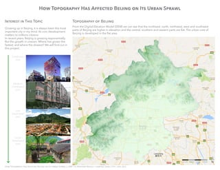
- 1. How Topography Has Affected Beijing on Its Urban Sprawl | LARP 743 Midterm Project | Jianting Zhao | Oct. 24th 2016 10 km 20 km 30km 40km n How Topography Has Affected Beijing on Its Urban Sprawl Interest in This Topic Growing up in Beijing, it is always been the most important city in my mind. Its civic development matters to millions citizens. In recent years, Beijing is growing exponentially. But the growth in uneven. Where has grown the fastest, and where the slowest? We will find out in this project. Topography of Beijing From the Digital Elevation Model (DEM) we can see that the northeast, north, northwest, west and southwest parts of Beijing are higher in elevation and the central, southern and eastern parts are flat. The urban core of Beijing is developed in the flat area. Developed area Medium Developed area Less Developed area Under Developed area
- 2. How Topography Has Affected Beijing on Its Urban Sprawl | LARP 743 Midterm Project | Jianting Zhao | Oct. 24th 2016 Urban Development Over 2 Decades The shapefiles of the urban sprawl from 1993 to 2012 and the Night Lighting from the same time span are displayed. There is a close relationship between urban sprawl and stable lights. However, the shapefiles are able to show urban development beyond Beijing as well, whereas their counterparts in lighting are clipped. Annual Urban Sprawl Annual Stable Lighting 1993 1994 1995 1996 1993 1994 1995 1996 1997 1998 1999 2000 1997 1998 1999 2000 2001 2002 2003 2004 2001 2002 2003 2004 2005 2006 2007 2008 2005 2006 2007 2008 2009 2010 2011 2012 2009 2010 2011 2012
- 3. How Topography Has Affected Beijing on Its Urban Sprawl | LARP 743 Midterm Project | Jianting Zhao | Oct. 24th 2016 Overlay Comparison Urban Sprawl Overlay from 1993-2012 It is apparent that the flatter area are occupied by people and development. More importantly, the urban sprawl also goes beyond Beijing’s municipal boundary towards east, southeast and south. Stable Lights Overlay from 1993-2012 The lighting overlay almost fills up the low elevation area in Beijing. The pattern is very similar to that of urban sprawl. It is easy to see a correlation between these two properties.
- 4. How Topography Has Affected Beijing on Its Urban Sprawl | LARP 743 Midterm Project | Jianting Zhao | Oct. 24th 2016 Rate of Urbanization After confirming the close relationship between urban sprawl shapefiles and stable lights images, I used the image collection to conduct further analysis, because there are more methods available to work with image collection in Google Earth Engine. Rate of Urbanization is calculated by adding the pixel values of each year and reducing to an image with the sum of all pixel values over time span (as shown below). The darker green indicates higher pixel value, and hence longer time of stable lights. Afterward, I reprojected this sum image to EPSG:3857 -- WGS84 Web Mercator (Auxiliary Sphere) projection. By doing this projection, I was able to use ee.Terrain.slope to calculate the slope of that sum image, such that I can get the rate of urbanization over 2 decades (Right Image). The slope is calculated such that the steeper slope (darker blue) represents less sprawl over unit time, versus flatter slope (lighter blue) indicates more sprawl over unit time. More Stable Light Faster Sprawl Less Stable Light Slower Sprawl The area in the mountain region has darker colors, indicating slow urban sprawl. In contrast, the area on plain has bigger urban sprawl.
- 5. How Topography Has Affected Beijing on Its Urban Sprawl | LARP 743 Midterm Project | Jianting Zhao | Oct. 24th 2016 Other Approaches of Analysis on Urbanization Summarizing Urban Sprawl by Standard Deviation Over 2 decades, the lighting has changed a lot, and it is in general, from low light intensity to high intensity. Therefore, one way to measure the urban sprawl is to measure how unstable the light intensity is over the years. If it is big, that means it’s been developing and vice versa. The central urban core has small number, because it is lit up throughout the time span, whereas the mountain area has small number because there isn’t much development. Summarizing Urban Sprawl by Mean This method produces similar result to the sum image. In this mean image, each pixel represents the mean value of stable light intensity over the time span. The urban core, where is always lit up, has the highest mean value, and the less development the less pixel value in the rest of the area. More Change In Light Intensity More Stable Light Less Change In Light Intensity Less Stable Light
- 6. How Topography Has Affected Beijing on Its Urban Sprawl | LARP 743 Midterm Project | Jianting Zhao | Oct. 24th 2016 /////////// Load Data ///////////////// var BJdem1 = ee.Image(“users/zhaojianting/MidTerm/ASTGTM2_N39E116_dem”), BJdem2 = ee.Image(“users/zhaojianting/MidTerm/ASTGTM2_N40E116_dem”), BJdem3 = ee.Image(“users/zhaojianting/MidTerm/ASTGTM2_N39E115_dem”), BJdem4 = ee.Image(“users/zhaojianting/MidTerm/ASTGTM2_N39E117_dem”), BJdem5 = ee.Image(“users/zhaojianting/MidTerm/ASTGTM2_N40E115_dem”), BJdem6 = ee.Image(“users/zhaojianting/MidTerm/ASTGTM2_N40E117_dem”), BJdem7 = ee.Image(“users/zhaojianting/MidTerm/ASTGTM2_N41E116_dem”), BJ = ee.FeatureCollection(“ft:1y1yODcot22kvYzeKKuZllMro1fkzSQf2ozfF0Qnw”), BJ1993 = ee.FeatureCollection(“ft:1Gr-KhI32ffFCDLgBKIIF9y2rkWQIMDp-zDqp8At4”), BJ1994 = ee.FeatureCollection(“ft:1oQeiBQIRoNgPEKeDZ1u8qCQP5I657fsOMecSZ0l-”), BJ1995 = ee.FeatureCollection(“ft:1Wf6L2ZbhZ1c3UQM95RVZzMsr8-ZHk1GmpSmN5OMd”), BJ1996 = ee.FeatureCollection(“ft:1us8xnLuzbc71qHphrL1lz-9_mSq_FSFLpxMNrKJz”), BJ1997 = ee.FeatureCollection(“ft:1sbnsmOV5Kb2fA5fXdB8Vq-Jr2NJRa0tCkNtdnPR4”), BJ1998 = ee.FeatureCollection(“ft:1r3DcuFbra-HMUOT8KzJgMfViYDmDC7St1PzFt-A8”), BJ1999 = ee.FeatureCollection(“ft:1DFfQ51IyxddakAXHQBg4uNsZobwRUDl-6G8sSuj_”), BJ2000 = ee.FeatureCollection(“ft:1LJIlkDNa3Xq4gH9ivO_8kWNVpKHZgsU5WLCfaI2u”), BJ2001 = ee.FeatureCollection(“ft:1fdungkkXjF4Qr-MQhAIfAMOME39-5GizAQeHqVZT”), BJ2002 = ee.FeatureCollection(“ft:1m2Qk089MtdxU3v6zk7fNQCvv0WpYstFKqapvrTEW”), BJ2003 = ee.FeatureCollection(“ft:1VnZiXbcHAeIu_aY1awpGCDIJWGD1-mgo8Op_gfjr”), BJ2004 = ee.FeatureCollection(“ft:17hXweCxsqYgqLt65MLWAzRMphpg61PBRrMPrljZy”), BJ2005 = ee.FeatureCollection(“ft:1dSrFSQNFnXZptJ8ilOepJ3yRDFEKO9gj9UFK1fcW”), BJ2006 = ee.FeatureCollection(“ft:1D7ALNyY8c6PIDGy_a15Tc6wb2y-77ZMArmI8EUuy”), BJ2007 = ee.FeatureCollection(“ft:15CCzRn4XCa0dRUgXlyvPMGwylF02DaCaw54ydRvr”), BJ2008 = ee.FeatureCollection(“ft:1D9OxIv6-nXzJ2idPHPX2lBuBZP8ZhyE-Y_6ekff8”), BJ2009 = ee.FeatureCollection(“ft:15Nfkm2ADzgduaPsE3iwMdiZZ6Zjuq9avoQerXgz0”), BJ2010 = ee.FeatureCollection(“ft:1lyLAs2x4JiyQCThmqbpbBq6whfuAAF0Jt17ogQpW”), BJ2011 = ee.FeatureCollection(“ft:13MPSOxUqk9hcm12kLa3sTHoJTapF2a4hrXqQdjb-”), BJ2012 = ee.FeatureCollection(“ft:1bXJ0xyWwGbM48KAQm6HdtDAPD5lzCN2CIVtg5I0n”), Lt1993 = ee.Image(“NOAA/DMSP-OLS/NIGHTTIME_LIGHTS/F101993”), Lt1994 = ee.Image(“NOAA/DMSP-OLS/NIGHTTIME_LIGHTS/F101994”), Lt1995 = ee.Image(“NOAA/DMSP-OLS/NIGHTTIME_LIGHTS/F121995”), Lt1996 = ee.Image(“NOAA/DMSP-OLS/NIGHTTIME_LIGHTS/F121996”), Lt1997 = ee.Image(“NOAA/DMSP-OLS/NIGHTTIME_LIGHTS/F121997”), Lt1998 = ee.Image(“NOAA/DMSP-OLS/NIGHTTIME_LIGHTS/F121998”), Lt1999 = ee.Image(“NOAA/DMSP-OLS/NIGHTTIME_LIGHTS/F121999”), Lt2000 = ee.Image(“NOAA/DMSP-OLS/NIGHTTIME_LIGHTS/F142000”), Lt2001 = ee.Image(“NOAA/DMSP-OLS/NIGHTTIME_LIGHTS/F142001”), Lt2002 = ee.Image(“NOAA/DMSP-OLS/NIGHTTIME_LIGHTS/F142002”), Lt2003 = ee.Image(“NOAA/DMSP-OLS/NIGHTTIME_LIGHTS/F142003”), Lt2004 = ee.Image(“NOAA/DMSP-OLS/NIGHTTIME_LIGHTS/F152004”), Lt2005 = ee.Image(“NOAA/DMSP-OLS/NIGHTTIME_LIGHTS/F152005”), Lt2006 = ee.Image(“NOAA/DMSP-OLS/NIGHTTIME_LIGHTS/F152006”), Lt2007 = ee.Image(“NOAA/DMSP-OLS/NIGHTTIME_LIGHTS/F152007”), Lt2008 = ee.Image(“NOAA/DMSP-OLS/NIGHTTIME_LIGHTS/F152008”), Lt2009 = ee.Image(“NOAA/DMSP-OLS/NIGHTTIME_LIGHTS/F162009”), Lt2010 = ee.Image(“NOAA/DMSP-OLS/NIGHTTIME_LIGHTS/F182010”), Lt2011 = ee.Image(“NOAA/DMSP-OLS/NIGHTTIME_LIGHTS/F182011”), Lt2012 = ee.Image(“NOAA/DMSP-OLS/NIGHTTIME_LIGHTS/F182012”); Google Earth Engine Code ---> Conclusion From the comparisons of topography and urban sprawl images, we can see a relationship between them. More mountains hinders urban sprawl. This makes sense because uneven topography makes urban development harder. People tend to gather on flat topography. For Beijing specifically, it is growing eastard and connecting with other larger cities such as Tangshan and Tianjin. If the sprawl keeps its pace, Beijing will become a giant metropolitan area expanding all the way to the Bohai Sea.
- 7. How Topography Has Affected Beijing on Its Urban Sprawl | LARP 743 Midterm Project | Jianting Zhao | Oct. 24th 2016 //////////////// Locate the map to Beijing ///////////////////////// Map.setCenter(116.4056, 39.9083,9); /////////////// Creating an Image Collection for DEM //////////////// var DEM_collection = ee.ImageCollection([BJdem1,BJdem2,BJdem3,BJdem4,BJdem5,BJdem6,BJdem7]); /////////////// Clip Global DEM to only Beijing ////////////////// function ShowElv(DemImage){ return DemImage.clip(BJ); } var topoBJ = DEM_collection.map(ShowElv); ////////////// Creating Elevation for elevation higher than 150m and within Beijing ////////// function ShowHighElv(DemImage){ var dem_mask = DemImage.gt(150); var high_elev = DemImage.mask(dem_mask); var high_elev_bj = high_elev.clip(BJ); return high_elev_bj; } var HIGHDEM_col = DEM_collection.map(ShowHighElv); //////// Clip night lighting to Beijing and mask out area without stable lighting or intensity less than 15 /// var NightLight = ee.ImageCollection([Lt1993,Lt1994,Lt1995,Lt1996,Lt1997,Lt1998,Lt1999,Lt2000, Lt2001,Lt2002,Lt2003,Lt2004,Lt2005,Lt2006,Lt2007,Lt2008,Lt2009,Lt2010,Lt2011,Lt2012]); print(‘night light’,NightLight); function LightBJ(LightImage){ var light_mask = LightImage.select([‘stable_lights’]).gt(15); var lightOn = LightImage.mask(light_mask); var lightOnBJ = lightOn.clip(BJ); return lightOnBJ; } var light_clip = NightLight.map(LightBJ); ////////////// Calculate Rate of Growth in Urban Area based on Night Lighting /////////////// function LightBJAll(LightImage){ var lightBJall = LightImage.clip(BJ); return lightBJall; } var lights_BJ = NightLight.map(LightBJAll) var light_sd = lights_BJ.select(‘stable_lights’).reduce(ee.Reducer.stdDev()); var light_mean = lights_BJ.select(‘stable_lights’).mean(); var light_sum = lights_BJ.select(‘stable_lights’).sum(); var light_sum_proj = light_sum.reproject(‘EPSG:3857’,null,1000); var urban_rate = ee.Terrain.slope(light_sum_proj); print(‘urban rate’, urban_rate); Google Earth Engine Code - continued
- 8. How Topography Has Affected Beijing on Its Urban Sprawl | LARP 743 Midterm Project | Jianting Zhao | Oct. 24th 2016 //////////// urban area shapefile bounded to BEIJING ////// var BJ1993_bound = BJ1993.filterBounds(BJ); var BJ1994_bound = BJ1994.filterBounds(BJ); var BJ1995_bound = BJ1995.filterBounds(BJ); var BJ1996_bound = BJ1996.filterBounds(BJ); var BJ1997_bound = BJ1997.filterBounds(BJ); var BJ1998_bound = BJ1998.filterBounds(BJ); var BJ1999_bound = BJ1999.filterBounds(BJ); var BJ2000_bound = BJ2000.filterBounds(BJ); var BJ2001_bound = BJ2001.filterBounds(BJ); var BJ2002_bound = BJ2002.filterBounds(BJ); var BJ2003_bound = BJ2003.filterBounds(BJ); var BJ2004_bound = BJ2004.filterBounds(BJ); var BJ2005_bound = BJ2005.filterBounds(BJ); var BJ2006_bound = BJ2006.filterBounds(BJ); var BJ2007_bound = BJ2007.filterBounds(BJ); var BJ2008_bound = BJ2008.filterBounds(BJ); var BJ2009_bound = BJ2009.filterBounds(BJ); var BJ2010_bound = BJ2010.filterBounds(BJ); var BJ2011_bound = BJ2011.filterBounds(BJ); var BJ2012_bound = BJ2012.filterBounds(BJ); ////////////// Show Beijing Topography /////////////////////////////////////////// Map.addLayer(topoBJ,{min:0, max: 2200,palette:[‘e6ffe6’,’006622’]},’BJ Topo’) ////////////// Present lighting for each year ////////////////// Map.addLayer(light_clip.filterDate(‘1993-01-01’,’1993-12-31’), {min:0,max:65,palette:[‘000000’,’ffffb3’], bands:’stable_lights’},’nightlights1993’); Map.addLayer(light_clip.filterDate(‘1994-01-01’,’1994-12-31’), {min:0,max:65,palette:[‘000000’,’ffffb3’], bands:’stable_lights’},’nightlights1994’); Map.addLayer(light_clip.filterDate(‘1995-01-01’,’1995-12-31’), {min:0,max:65,palette:[‘000000’,’ffffb3’], bands:’stable_lights’},’nightlights1995’); Map.addLayer(light_clip.filterDate(‘1996-01-01’,’1996-12-31’), {min:0,max:65,palette:[‘000000’,’ffffb3’], bands:’stable_lights’},’nightlights1996’); Map.addLayer(light_clip.filterDate(‘1997-01-01’,’1997-12-31’), {min:0,max:65,palette:[‘000000’,’ffffb3’], bands:’stable_lights’},’nightlights1997’); Map.addLayer(light_clip.filterDate(‘1998-01-01’,’1998-12-31’), {min:0,max:65,palette:[‘000000’,’ffffb3’], bands:’stable_lights’},’nightlights1998’); Map.addLayer(light_clip.filterDate(‘1999-01-01’,’1999-12-31’), {min:0,max:65,palette:[‘000000’,’ffffb3’], bands:’stable_lights’},’nightlights1999’); Map.addLayer(light_clip.filterDate(‘2000-01-01’,’2000-12-31’), {min:0,max:65,palette:[‘000000’,’ffffb3’], bands:’stable_lights’},’nightlights2000’); Map.addLayer(light_clip.filterDate(‘2001-01-01’,’2001-12-31’), {min:0,max:65,palette:[‘000000’,’ffffb3’], bands:’stable_lights’},’nightlights2001’); Google Earth Engine Code - continued
- 9. How Topography Has Affected Beijing on Its Urban Sprawl | LARP 743 Midterm Project | Jianting Zhao | Oct. 24th 2016 Map.addLayer(light_clip.filterDate(‘2002-01-01’,’2002-12-31’), {min:0,max:65,palette:[‘000000’,’ffffb3’], bands:’stable_lights’},’nightlights2002’); Map.addLayer(light_clip.filterDate(‘2003-01-01’,’2003-12-31’), {min:0,max:65,palette:[‘000000’,’ffffb3’], bands:’stable_lights’},’nightlights2003’); Map.addLayer(light_clip.filterDate(‘2004-01-01’,’2004-12-31’), {min:0,max:65,palette:[‘000000’,’ffffb3’], bands:’stable_lights’},’nightlights2004’); Map.addLayer(light_clip.filterDate(‘2005-01-01’,’2005-12-31’), {min:0,max:65,palette:[‘000000’,’ffffb3’], bands:’stable_lights’},’nightlights2005’); Map.addLayer(light_clip.filterDate(‘2006-01-01’,’2006-12-31’), {min:0,max:65,palette:[‘000000’,’ffffb3’], bands:’stable_lights’},’nightlights2006’); Map.addLayer(light_clip.filterDate(‘2007-01-01’,’2007-12-31’), {min:0,max:65,palette:[‘000000’,’ffffb3’], bands:’stable_lights’},’nightlights2007’); Map.addLayer(light_clip.filterDate(‘2008-01-01’,’2008-12-31’), {min:0,max:65,palette:[‘000000’,’ffffb3’], bands:’stable_lights’},’nightlights2008’); Map.addLayer(light_clip.filterDate(‘2009-01-01’,’2009-12-31’), {min:0,max:65,palette:[‘000000’,’ffffb3’], bands:’stable_lights’},’nightlights2009’); Map.addLayer(light_clip.filterDate(‘2010-01-01’,’2010-12-31’), {min:0,max:65,palette:[‘000000’,’ffffb3’], bands:’stable_lights’},’nightlights2010’); Map.addLayer(light_clip.filterDate(‘2011-01-01’,’2011-12-31’), {min:0,max:65,palette:[‘000000’,’ffffb3’], bands:’stable_lights’},’nightlights2011’); Map.addLayer(light_clip.filterDate(‘2012-01-01’,’2012-12-31’), {min:0,max:65,palette:[‘000000’,’ffffb3’], bands:’stable_lights’},’nightlights2012’); ///////////////// Show Annual Urban Development /////////////////////// Map.addLayer(BJ1993_bound, {color:’1a8cff’}, ‘BJ 1993’); Map.addLayer(BJ1994_bound, {color:’1a8cff’}, ‘BJ 1994’); Map.addLayer(BJ1995_bound, {color: ‘1a8cff’}, ‘BJ 1995’); Map.addLayer(BJ1996_bound, {color: ‘1a8cff’}, ‘BJ 1996’); Map.addLayer(BJ1997_bound, {color: ‘1a8cff’}, ‘BJ 1997’); Map.addLayer(BJ1998_bound, {color: ‘1a8cff’}, ‘BJ 1998’); Map.addLayer(BJ1999_bound, {color: ‘1a8cff’}, ‘BJ 1999’); Map.addLayer(BJ2000_bound, {color: ‘1a8cff’}, ‘BJ 2000’); Map.addLayer(BJ2001_bound, {color: ‘1a8cff’}, ‘BJ 2001’); Map.addLayer(BJ2002_bound, {color: ‘1a8cff’}, ‘BJ 2002’); Map.addLayer(BJ2003_bound, {color: ‘1a8cff’}, ‘BJ 2003’); Map.addLayer(BJ2004_bound, {color: ‘1a8cff’}, ‘BJ 2004’); Map.addLayer(BJ2005_bound, {color: ‘1a8cff’}, ‘BJ 2005’); Map.addLayer(BJ2006_bound, {color: ‘1a8cff’}, ‘BJ 2006’); Map.addLayer(BJ2007_bound, {color: ‘1a8cff’}, ‘BJ 2007’); Map.addLayer(BJ2008_bound, {color: ‘1a8cff’}, ‘BJ 2008’); Map.addLayer(BJ2009_bound, {color: ‘1a8cff’}, ‘BJ 2009’); Map.addLayer(BJ2010_bound, {color: ‘1a8cff’}, ‘BJ 2010’); Map.addLayer(BJ2011_bound, {color: ‘1a8cff’}, ‘BJ 2011’); Map.addLayer(BJ2012_bound, {color: ‘1a8cff’}, ‘BJ 2012’); Google Earth Engine Code - continued
- 10. How Topography Has Affected Beijing on Its Urban Sprawl | LARP 743 Midterm Project | Jianting Zhao | Oct. 24th 2016 ////////////// Show Urbanization Rate, darker color means slower sprawl, vice versa ///////// Map.addLayer(urban_rate,{min:0,max:20,palette:[‘e6f9ff’,’0099cc’] },’Urbanization Rate’); ///////////// Show Mountains of Beijing ////////////////////////// Map.addLayer(HIGHDEM_col,{min:150, max: 2200,palette:[‘e6ffe6’,’006622’]},’BJ mountain’) ///////////// Show other statistics measuring of lights over 2 decades ////////////// Map.addLayer(light_sd,{min:0,max:20,palette:[‘ecffb3’,’739900’]},’light value sd’); Map.addLayer(light_mean,{min:0,max:65,palette:[‘ecffb3’,’739900’]},’Light mean value’); Map.addLayer(light_sum,{min:0,max:1500,palette:[‘ecffb3’,’739900’]},’Light sum value’); ///////////// Show other statistics measuring of lights over 2 decades ////////////// Map.addLayer(light_sd,{min:0,max:20,palette:[‘ecffb3’,’739900’]},’light value sd’); Map.addLayer(light_mean,{min:0,max:65,palette:[‘ecffb3’,’739900’]},’Light mean value’); Map.addLayer(light_sum,{min:0,max:1500,palette:[‘ecffb3’,’739900’]},’Light sum value’); Google Earth Engine Code - continued
- 11. How Topography Has Affected Beijing on Its Urban Sprawl | LARP 743 Midterm Project | Jianting Zhao | Oct. 24th 2016 Data Sources: USGS Earth Explorer: http://earthexplorer.usgs.gov/ Beijing City Lab: http://www.beijingcitylab.com/data-released-1/ NOAA Night Light: https://code.earthengine.google.com/ ArcGIS tutorial: http://desktop.arcgis.com/en/arcmap/10.3/tools/spatial-analyst-toolbox/slope.htm Spatial Reference: http://spatialreference.org/ref/sr-org/7483/ Google Earth Engine Tutorial: https://developers.google.com/earth-engine Thank to Professor Dana Tomlin and Jill Kelly for technical support. Reference and Notes