Zhao,Jianting13ArcPy
•
0 likes•92 views

This document summarizes a project to redefine the bike score for Philadelphia using new metrics. The author conducted analyses on slope, tree density, intersection controls and bike lane types to calculate individual scores for each factor. The scores were combined to produce an overall bike score for each street segment. ArcPy scripts were used to perform spatial analyses and calculate the metrics from GIS data layers. The final tool allows users to input a location and get the bike score as well as scores for each individual factor.

Recommended
Recommended
More Related Content
Similar to Zhao,Jianting13ArcPy
Similar to Zhao,Jianting13ArcPy (20)
Zhao,Jianting13ArcPy
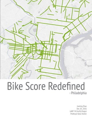
- 1. Bike Score Redefined-Philadelphia Jianting Zhao Dec 20 ,2016 LARP 743 ArcPy Project Professor Dana Tomlin
- 2. I. Introduction My interest in conducting a bike score evaluation for Philadelphia stems from my enthusiasm in biking. Before coming to Philadelphia, I know that Philadelphia is a car-independent city, meaning that people mostly do not need a car to get around especially in the downtown. So I imagined that it might as well be a bike friendly city, because if people do not drive, what would the other alternative be? Bike.To confirm with my assumption, I also looked up the bike score on Walkscore.com, a website that specializes in evaluating urban conditions, and a few other sources.As Walkscore says, the bike score in central Philadelphia is in the upper 80s, i.e. very bikeable (Figure 1). Philadelphia is also ranked high in the most bike friendly cities in the U.S. by other sources. Figure 1.Bike Score Report from Walkscore.com (Left-Top) Figure 2.Neighborhood Ranking from movoto.com (Left-Bottom) Figure 3.News from phillymag.com (Right-Top) Figure 4.Bike Score Ranking from forbes.com (Right-Middle) Figure 5.Bikeable Streets Ranking from Redfin.com (Right-Bottom)
- 3. However, as I tried a few times biking in the downtown area, the experience was not smooth.There are too many cars, very frequent signal controls, disconnected bike lanes, occupied bike lanes and etc.All these factors undermine bikers’ experience on streets. So I started to wonder why there is a discrepancy in scoring and the actual experience. I looked at the metrics Walkscore.com used to provide scores. It shows that they only take four criteria into account (Figure 6): Bike Lanes, Hills, Destination and road connectivity and Bike commuting mode share.And these criteria are evenly weighted, which may be inaccurate.The criteria from movoto.com leverages on bike score to make the bike- friendliness ranking, and focuses more on the infrastructure aspect, not the bikers’ experience. However, I Figure 6.Methodology from Walkscore.com Figure 7.Methodology from movoto.com believe the most important criteria are: the type of bike lane, width of bike lane, bike network connectivity, adjacent lane average car speed, density of trees, frequency of intersections. Due to absences of data in car speed, bike lane width and other variables, I was only able to measure the slope, tree density, intersection control density and bike lane types. I came up with the following metrics and ArcPy script to conduct a REDEFINED bike score evaluation. As an end product, this arcpy tool enables users to enter a longitude and latitude pair of a desired location, and this tool will return the bike score as well as the tree score, slope score, lane score and control score.
- 4. II. Methodology 0. Data Preparation and Cleaning Data sources are mostly from opendataphilly.org.The DEM model is retrieved from USGS Earth Explorer. Below is a list of datasets that I employed in my analysis: a. PhillyStreets_Street_Centerline.shp b. Bike_Network.shp c. DEM_Philly.tif d. PPR_StreetTrees.shp e. Intersection_Controls.shp As the base layer, PhillyStreets_Street_Centerline.shp contains all types of streets for the entire City of Philadelphia, ranging from small roads to highways. I cleaned it up by removing the “high speed ramp”, “highway”, “regional” and “boarder” street types, due to the fact that they are not bikeable by their nature.This still leaves most of the street on map (Figure 8). Code: ###### STEP 1 ## SELECT ONLY BIKEABLE STREETS FROM PHILLY_STREET_CENTERLINE InputLayer = r’C:UsersKristen ZhaoDocuments2016_UPennMUSA07_Data_L’ ‘ibPhiladelphiaDataPhillyStreets_Street_CenterlinePhillyStreets_Street_ Centerline.shp’ OutputShp = ‘Filtered_St2.shp’ arcpy.AddMessage(‘Input File is: ‘ + str(InputLayer)) arcpy.AddMessage(‘Output File is: ‘ + str(OutputShp)) query_clause = ‘CLASS IN (2,3,4,5,6,9,15)’ arcpy.MakeFeatureLayer_management(InputLayer, ‘StreetQueried’, query_clause) arcpy.CopyFeatures_management(‘StreetQueried’,OutputShp) 1. Metrics For all metrics, I scale them in different weights, and each of the metrics is scored using a 100 scale.The total bike score is also on a 100 scale.The scoring formula is as shown below: Bike Score = Lane_Type_Score * 0.5 + Slope_Score * 0.3 + Tree_Score * 0.1 + ControlsScore * 0.1 Code: ###### STEP 9 ## CALCULATE FINAL BIKE SCORE ############################ arcpy.AddField_management(‘StLaneSlopeTreeCtrl. shp’,’FinalScore’,’DOUBLE’,20,10) arcpy.CalculateField_management(‘StLaneSlopeTreeCtrl.shp’,’FinalScore’, ‘!SlopeScore!*0.3+!LaneScore!*0.5+!TreeScore!*0.1+!CtrlScore!*0.1’,’PYTHON_9.3’) For the Bike_Network.shp, there are several types of lane types included.They are a combination of sharrows, conventional, buffered and contraflow. For the definition of each term, please refer to this source: http://www. peopleforbikes.org/blog/entry/a-field-guide-to-north-american-bike-lanes. For all lane types in the dataset, I gave each a score, based on its perceived safeness and convenience. In general, a buffered bike lane is scored higher than a conventional, then sharrow and then contraflow.Also, two way bike lane is scored higher than one ways.There is no 100 score, because this Bike_Network unfortunately does not include separated bike trails which is the most ideal type for bikers.Thus, the score only goes up to 90.
- 5. Figure 8.Basemap of streets
- 6. In addition, there are many streets do not have a bike lane of any type, but I still consider them bikeable. But their score only goes to 30. Below is the scoring rubric: Type Score NULL 30 Sharrow 40 Conventional 50 Conventional with Sharrow 60 Contraflow with Conventional 70 Buffered 80 Buffered with Conventional 90 Code: ###### STEP 3 ## ADD FIELD IN NEW SHAPEFILE AND RECODE BIKE LANE TYPES FROM TEXT TO NUMERICS ########### arcpy.AddField_management(StBike_j, ‘LaneScore’, “SHORT”, 2) enumerationOfRecords = arcpy.UpdateCursor(‘StBike_j.shp’) for row in enumerationOfRecords: Type = row.getValue(‘TYPE’) if Type == ‘Sharrow’: row.setValue(‘LaneScore’,40) enumerationOfRecords.updateRow(row) elif Type == ‘Conventional’: row.setValue(‘LaneScore’,50) enumerationOfRecords.updateRow(row) elif Type == ‘Conventional w Sharrows’: row.setValue(‘LaneScore’,60) enumerationOfRecords.updateRow(row) elif Type == ‘Contraflow w Conventional, same’: row.setValue(‘LaneScore’,70) enumerationOfRecords.updateRow(row) elif Type == ‘Buffered’: row.setValue(‘LaneScore’,80) enumerationOfRecords.updateRow(row) elif Type == ‘Buffered w Conventional’: row.setValue(‘LaneScore’,90) enumerationOfRecords.updateRow(row) else: row.setValue(‘LaneScore’,30) enumerationOfRecords.updateRow(row) # Add a blank line at the bottom of the printed list arcpy.AddMessage(‘Success’) # Delete row and update cursor objects to avoid locking attribute table del row del enumerationOfRecords The second factor is slope steepness.As the article from https://www.bicyclenetwork.com.au/general/for- government-and-business/2864/ says, any slope steeper than 5% is going to be difficult for bikers in long distance.The ideal steepness range is from 0-5%, difficult range is 5-10% and impossible range is > 10%. Therefore, I coded the steepness score as below: Slope (%) Score 0-1 100 1.1-2 90 2.1-3 80 3.1-4 70 4.1-5 60 5.1-6 50
- 7. 6.1-7 40 7.1-8 30 8.1-9 20 9.1-10 10 > 10.1 0 Code: arcpy.AddField_management(‘StBikeSlope_j.shp’, ‘SlopeScore’, “SHORT”, 2) enumerationOfRecords2 = arcpy.UpdateCursor(‘StBikeSlope_j.shp’) for seg in enumerationOfRecords2: PctSlope = seg.getValue(‘MEAN’) #arcpy.AddMessage(‘type field is showing: ‘+ str(Type)) if PctSlope <= 1: seg.setValue(‘SlopeScore’,100) enumerationOfRecords2.updateRow(seg) elif PctSlope > 1 and PctSlope <= 2: seg.setValue(‘SlopeScore’,90) enumerationOfRecords2.updateRow(seg) elif PctSlope > 2 and PctSlope <= 3: seg.setValue(‘SlopeScore’,80) enumerationOfRecords2.updateRow(seg) elif PctSlope >3 and PctSlope <= 4: seg.setValue(‘SlopeScore’,70) enumerationOfRecords2.updateRow(seg) elif PctSlope >4 and PctSlope <= 5: seg.setValue(‘SlopeScore’,60) enumerationOfRecords2.updateRow(seg) elif PctSlope > 5 and PctSlope <= 6: seg.setValue(‘SlopeScore’,50) enumerationOfRecords2.updateRow(seg) elif PctSlope > 6 and PctSlope <= 7: seg.setValue(‘SlopeScore’,40) enumerationOfRecords2.updateRow(seg) elif PctSlope > 7 and PctSlope <= 8: seg.setValue(‘SlopeScore’,30) enumerationOfRecords2.updateRow(seg) elif PctSlope > 8 and PctSlope <= 9: seg.setValue(‘SlopeScore’,20) enumerationOfRecords2.updateRow(seg) elif PctSlope > 9 and PctSlope <= 10: seg.setValue(‘SlopeScore’,10) enumerationOfRecords2.updateRow(seg) else: seg.setValue(‘SlopeScore’,0) enumerationOfRecords2.updateRow(seg) #arcpy.AddMessage(“LaneScore = “ + str(row.getValue(‘LaneScore’))) # Add a blank line at the bottom of the printed list arcpy.AddMessage(‘Success’) # Delete row and update cursor objects to avoid locking attribute table del seg del enumerationOfRecords2 The third factor is Tree Density Score. I first calculated tree density by dividing number of trees on one street segment by the street length, such that I get number of trees per ft. I gave score by the following formula: Tree_Score = (observed tree density - min tree density) / (max tree density - min tree density) *100 Code: ###### STEP 6 ## CALCULATE TREE SCORE FOR STREETS ####################### ## PART 1 ## ADD FIELD FOR CALCULATING TREE DENSITY ###########
- 8. arcpy.AddField_management(‘StLaneSlopeTree.shp’, ‘TreeDs’, “DOUBLE”, 20,10) arcpy.CalculateField_management(‘StLaneSlopeTree. shp’,’TreeDs’,’!TreeCount!/!LENGTH!’,”PYTHON_9.3”) ## PART 2 ## CALCULATE SCORE BY COMPARING TREE DENSITY ########### arcpy.AddField_management(‘StLaneSlopeTree.shp’, ‘TreeScore’, “DOUBLE”, 20,10) minValue = arcpy.SearchCursor(‘StLaneSlopeTree.shp’, “”, “”, “”, ‘TreeDs’ + “ A”).next().getValue(‘TreeDs’) #Get 1st row in ascending cursor sort maxValue = arcpy.SearchCursor(‘StLaneSlopeTree.shp’, “”, “”, “”, ‘TreeDs’ + “ D”).next().getValue(‘TreeDs’) #Get 1st row in descending cursor sort pct = (maxValue - minValue) / 100 arcpy.AddMessage(‘pct is: ‘ + str(pct)) enumerationOfRecords3 = arcpy.UpdateCursor(‘StLaneSlopeTree.shp’) for seg in enumerationOfRecords3: TreeDsField = seg.getValue(‘TreeDs’) TrScoreCalc = TreeDsField / pct TreeScoreField = seg.setValue(‘TreeScore’,TrScoreCalc) enumerationOfRecords3.updateRow(seg) del seg del enumerationOfRecords3 The last factor, intersection control density is calculated in a similar manner, but since less intersection is better, the intersection density is calculated by street segment length divided by number of intersection controls on that segment.When there is no intersection control on a street segment, the 0 count is set to 1 in order to get real numbers.Afterward, the control score is calculated as below: Ctrl_Score = (observed Ctrl density - min ctrl density) / (max ctrl density - min ctrl density) *100 Code: ###### STEP 8 ## CALCULATE INTERSECTION CONTROL SCORES #################### ## PART 1 ## ADD FIELD FOR CALCULATING TREE DENSITY ########### arcpy.AddField_management(‘StLaneSlopeTreeCtrl.shp’, ‘CtrlDs’, “DOUBLE”, 20,10) enumerationOfRecords4 = arcpy.UpdateCursor(‘StLaneSlopeTreeCtrl.shp’) for seg in enumerationOfRecords4: stops = seg.getValue(‘STOPCount’) if stops == 0: newstops = seg.setValue(‘STOPCount’,1) enumerationOfRecords4.updateRow(seg) del enumerationOfRecords4 del seg arcpy.CalculateField_management(‘StLaneSlopeTreeCtrl. shp’,’CtrlDs’,’!STOPCount!/!LENGTH!’,”PYTHON_9.3”) ## PART 2 ## CALCULATE SCORE BY COMPARING TREE DENSITY ########### arcpy.AddField_management(‘StLaneSlopeTreeCtrl.shp’, ‘CtrlScore’, “DOUBLE”, 20,10) minValue = arcpy.SearchCursor(‘StLaneSlopeTreeCtrl.shp’, “”, “”, “”, ‘CtrlDs’ + “ A”).next().getValue(‘CtrlDs’) #Get 1st row in ascending cursor sort maxValue = arcpy.SearchCursor(‘StLaneSlopeTreeCtrl.shp’, “”, “”, “”, ‘CtrlDs’ + “ D”).next().getValue(‘CtrlDs’) #Get 1st row in descending cursor sort enumerationOfRecords5 = arcpy.UpdateCursor(‘StLaneSlopeTreeCtrl.shp’) for seg in enumerationOfRecords5: CtrlDsField = seg.getValue(‘CtrlDs’) CtrlScoreCalc = (CtrlDsField - minValue)/(maxValue - minValue) * 100 CtrlScoreField = seg.setValue(‘CtrlScore’,CtrlScoreCalc) enumerationOfRecords5.updateRow(seg) del seg del enumerationOfRecords5
- 9. 2.The processes to get the scores First let’s talk about the Bike Lane Type dataset. I found this dataset to share a common field with the overall street shapefile, that is “SEG_ID”.Therefore, I conducted tabular join to merge the bike network into street shapefile. Then, I recoded the scores as showed earlier in section1. Code: ###### STEP 2 ## TABULAR JOIN BIKENETWORK TO FILTERED_ST1 ## FIRST TO MAKE SHAPEFILEs INTO LAYER arcpy.MakeFeatureLayer_management(‘Filtered_St2.shp’, “FilteredSt_lyr”) JoinFeature = ‘BikeNetwork_Proj.shp’ arcpy.AddMessage(‘Input bike network is: ‘ + str(JoinFeature)) ## JOIN TWO LAYERS arcpy.AddJoin_management(‘FilteredSt_lyr’,’SEG_ID’,JoinFeature,’SEG_ID’) StBike_j = arcpy.CopyFeatures_management(‘FilteredSt_lyr’, ‘StBike_j.shp’) The second dataset is the DEM model. Prior to this project, the DEMs have already been stitched together and extracted by Philadelphia’s boundary and ready for use. In this project, I conducted slope analysis on this Philadelphia DEM dataset, and followed by a zonal statistics as table analysis to convert rasters into something that can by attached to the street shapefile. People may question if the slope is accurate given that I conducted it on a line shapefile. I thought about buffering the street to its actual width, however, since each street is its segment, there could be lots of overlaps at right corners. I thought that since the slope across each street section is quite uniform, street center line should be representative to the streets with width. Code: ###### STEP 4 ## GET SLOPE FOR EACH STREET SEGMENT ############ ## PART 1 ## GET SLOPE FROM MASKED DEM OF PHILLY InputDEM = r’C:UsersKristen ZhaoDocuments2016_UPennMUSA07_Data_Lib PhiladelphiaDataphiladem2’ PhilaSlope = arcpy.sa.Slope(InputDEM, ‘PERCENT_RISE’) PhilaSlope.save(‘PhilaSlope’) # save slope file ## PART 2 ## GET AVERAGE SLOPE FOR EACH LINE SEGMENT ########## # ZONAL STATISTICS AS TABLE SlopeByStreet = arcpy.sa.ZonalStatisticsAsTable(‘StBike_j.shp’, ‘SEG_ID’, ‘PhilaSlope’, ‘SlopeByStreet. dbf’, ‘DATA’, ‘MEAN’) # JOIN TO CREATE StBikeSlope_j.shp arcpy.MakeFeatureLayer_management(‘StBike_j.shp’, “StBike_lyr”) arcpy.AddJoin_management(‘StBike_lyr’,’SEG_ID’,’SlopebyStreet.dbf’,’SEG_ID’) StBikeSlope_j = arcpy.CopyFeatures_management(‘StBike_lyr’, ‘StBikeSlope_j. shp’) # DELETE UNUSEFUL FIELDS AND CONVERT SLOPE (MEAN FIELD) INTO SLOPE SCORES arcpy.DeleteField_management(‘StBikeSlope_j.shp’,[‘SEG_ ID_12’,’OID_’,’COUNT’,’AREA’,’SHAPE_Leng’,’FID_1’,’OBJECTID’,’SEG_ID1’]) The third dataset is PPR_StreetTree.shp. I conducted a spatial join to join trees that are close to a street segment to that street segment.The difficulty here was that the tree points are not perfectly on top of the street lines.Thus I need to create a field mapping and search for trees around the street segments. Code: ###### STEP 5 ## SPATIAL JOIN STREET TREES TO StBikeSlope_j.shp ########### ## PART 1 ## CONVERT SHAPEFILES TO LAYERS ##### arcpy.MakeFeatureLayer_management(‘StBikeSlope_j.shp’, “StBikeSlope_lyr”) arcpy.MakeFeatureLayer_management(r’C:UsersKristen ZhaoDocuments2016_ UPennMUSA07_Data_LibPhiladelphiaDataPPR_StreetTreesPPR_StreetTrees.shp’, “StreetTree_lyr”) ## PART 2 ## SET UP FIELD MAPPING #############
- 10. # Create a new fieldmappings and add the two input feature classes. fieldmappingsTree = arcpy.FieldMappings() fieldmappingsTree.addTable(‘StBikeSlope_lyr’) fieldmappingsTree.addTable(‘StreetTree_lyr’) TreeFieldIndex = fieldmappingsTree.findFieldMapIndex(“OBJECTID”) fieldmapTree = fieldmappingsTree.getFieldMap(TreeFieldIndex) # Get the output field’s properties as a field object fieldTree = fieldmapTree.outputField # Rename the field and pass the updated field object back into the field map fieldTree.name = “TreeCount” fieldTree.aliasName = “TreeCount” fieldmapTree.outputField = fieldTree # Set the merge rule and then replace the old fieldmap in the mappings object # with the updated one fieldmapTree.mergeRule = “Count” fieldmappingsTree.replaceFieldMap(TreeFieldIndex, fieldmapTree) # Delete fields that are no longer applicable # as only the first value will be used by default y = fieldmappingsTree.findFieldMapIndex(“SPECIES”) fieldmappingsTree.removeFieldMap(y) z = fieldmappingsTree.findFieldMapIndex(“STATUS”) fieldmappingsTree.removeFieldMap(z) w = fieldmappingsTree.findFieldMapIndex(“DBH”) fieldmappingsTree.removeFieldMap(w) ## PART 3 ## CONDUCT SPATIAL JOIN TO FORM NEW SHAPEFILE StLaneSlopeTree.shp arcpy.SpatialJoin_analysis(‘StBikeSlope_lyr’, ‘StreetTree_lyr’, ‘StLaneSlopeTree.shp’, ‘JOIN_ONE_TO_ONE’, ‘KEEP_ALL’, fieldmappingsTree, ‘WITHIN_A_DISTANCE’, ‘30 feet’) The last file is the Intersection_Control.shp. Similar to the tree file, I spatial joined it to street file. Code: ###### STEP 7 ## SPATIAL JOIN INTERSECTIONS TO STREETS ################## ## PART 1 ## CONVERT SHAPEFILES TO LAYERS ##### arcpy.MakeFeatureLayer_management(‘StLaneSlopeTree.shp’, “StLaneSlopeTree_ lyr”) arcpy.MakeFeatureLayer_management(r’C:UsersKristen ZhaoDocuments2016_ UPennMUSA07_Data_LibPhiladelphiaDataIntersection_Controls.shp’, “STOP_lyr”) ## PART 2 ## SET UP FIELD MAPPING ############# # Create a new fieldmappings and add the two input feature classes. fieldmappingsSTOP = arcpy.FieldMappings() fieldmappingsSTOP.addTable(‘StLaneSlopeTree_lyr’) fieldmappingsSTOP.addTable(‘STOP_lyr’) # for the output. STOPFieldIndex = fieldmappingsSTOP.findFieldMapIndex(“OBJECTID”) fieldmapSTOP = fieldmappingsSTOP.getFieldMap(STOPFieldIndex) # Get the output field’s properties as a field object fieldSTOP = fieldmapSTOP.outputField # Rename the field and pass the updated field object back into the field map fieldSTOP.name = “STOPCount” fieldSTOP.aliasName = “STOPCount” fieldmapSTOP.outputField = fieldSTOP # Set the merge rule and then replace the old fieldmap in the mappings object # with the updated one fieldmapSTOP.mergeRule = “Count”
- 11. fieldmappingsSTOP.replaceFieldMap(STOPFieldIndex, fieldmapSTOP) # Delete fields that are no longer applicable # as only the first value will be used by default y = fieldmappingsSTOP.findFieldMapIndex(“NODE_ID”) fieldmappingsSTOP.removeFieldMap(y) ## PART 3 ## CONDUCT SPATIAL JOIN TO FORM NEW SHAPEFILE StLaneSlopeTree.shp ############## #Run the Spatial Join tool, using the defaults for the join operation and join type arcpy.SpatialJoin_analysis(‘StLaneSlopeTree_lyr’, ‘STOP_lyr’, ‘StLaneSlopeTreeCtrl.shp’, ‘JOIN_ONE_TO_ONE’, ‘KEEP_ALL’, fieldmappingsSTOP, ‘WITHIN_A_DISTANCE’, ‘10 feet’) 3. User Input and Feedback Let’s set aside the score, and think about the use of this tool. I wanted it to be a tool that people can query the bike score of an area.Therefore, I need some kind of user input and output. I designed this to be capable of accepting longitude and latitude coordinates (figure 9). Once user enters the information, this tool will be able to identify the point and retrieve the average score of the area with a search radius of 3000 feet.The coordinates is easy to get by going into this address longlat converter website: http://www.latlong.net/convert-address-to- lat-long.html. The reason for not using an address, which would presumably be easier to use, is that I encountered technical difficulty to geocode addresses successfully between two different address locator styles. More would be discussed at the discussion section. Code: ###### STEP 10 ## CREATE GEOLOCATOR ####################### ‘’’ DISPLAY NAME DATA TYPE PROPERTY>DIRECTION>VALUE Input Longitude Double Input Input Latitude Double Unput Output Shapefile Shapefile Output example: 3600 Chestnut St ‘’’ ## PART 0 ## GET SPATIAL REFERENCE ####################### spatialref = arcpy.SpatialReference(‘WGS 1984’) arcpy.AddMessage(‘spatital reference is: ‘ + str(spatialref)) ## PART 1 ## CREATE A TABLE TO STORE USER SPECIFIED ADDRESS ########### nameOfInputLat = arcpy.GetParameterAsText(0) arcpy.AddMessage(‘n’ + “The input layer name is “ + nameOfInputLat) nameOfInputLong = arcpy.GetParameterAsText(1) arcpy.AddMessage(‘n’ + “The input layer name is “ + nameOfInputLong) nameOfOutputShp = arcpy.GetParameterAsText(2) arcpy.AddMessage(“The output shapefile name is “ + nameOfOutputShp) arcpy.CreateTable_management (r’C:UsersKristen ZhaoDocuments2016_ UPennMUSA04_Courses02_LARP_743FinalProjNewLayers’, ‘Coordinates.dbf’) arcpy.AddField_management(‘Coordinates.dbf’,’Latitude’,’DOUBLE’,20,10) arcpy.AddField_management(‘Coordinates.dbf’,’Longitude’,’DOUBLE’,20,10) coords = arcpy.InsertCursor(‘Coordinates.dbf’) inputCoords = coords.newRow() inputCoords.setValue(‘Latitude’,nameOfInputLong) inputCoords.setValue(‘Longitude’,nameOfInputLat) coords.insertRow(inputCoords) del inputCoords del coords ## PART 2 ## CREATE POINT FROM LAT LONG ############# arcpy.MakeXYEventLayer_management (‘Coordinates.dbf’, ‘Latitude’, ‘Longitude’, ‘Address’, spatialref)
- 12. arcpy.CopyFeatures_management(‘Address’,’UserLocation.shp’) ###### STEP 11 ## CREATE SUMMARY FOR USER SPECIFIED LOCATION ############# ## PART 1 ## CONVERT SHAPEFILES TO LAYERS ##### arcpy.MakeFeatureLayer_management(‘StLaneSlopeTreeCtrl.shp’, “Score_lyr”) arcpy.MakeFeatureLayer_management(‘UserLocation.shp’, “Location_lyr”) ## PART 2 ## SPATIAL JOIN THE POINT TO BIKESCORE SHAPEFILE ############## # Create a new fieldmappings and add the two input feature classes. fieldmappingsSCORE = arcpy.FieldMappings() fieldmappingsSCORE.addTable(‘Location_lyr’) fieldmappingsSCORE.addTable(‘Score_lyr’) SCOREFieldIndex = fieldmappingsSCORE.findFieldMapIndex(“FinalScore”) fieldmapSCORE = fieldmappingsSCORE.getFieldMap(SCOREFieldIndex) # Get the output field’s properties as a field object fieldSCORE = fieldmapSCORE.outputField # Rename the field and pass the updated field object back into the field map fieldSCORE.name = “FinalScore” fieldSCORE.aliasName = “FinalScore” fieldmapSCORE.outputField = fieldSCORE # Set the merge rule and then replace the old fieldmap in the mappings object # with the updated one fieldmapSCORE.mergeRule = “Mean” fieldmappingsSCORE.replaceFieldMap(SCOREFieldIndex, fieldmapSCORE) # Name fields you want. Could get these names programmatically too. keepers = [“eScore”, “SlopeScore”, “TreeScore”,”CtrlScore”,’FinalScore’] # Remove all output fields you don’t want. for field in fieldmappingsSCORE.fields: if field.name not in keepers: fieldmappingsSCORE.removeFieldMap(fieldmappingsSCORE. findFieldMapIndex(field.name)) ## PART 3 ## CONDUCT SPATIAL JOIN TO CREATE SCORE SUMMARY ############## arcpy.SpatialJoin_analysis(‘Location_lyr’, ‘Score_lyr’, nameOfOutputShp, ‘JOIN_ONE_TO_ONE’, ‘KEEP_COMMON’, fieldmappingsSCORE, ‘WITHIN_A_DISTANCE’, ‘3000 feet’) Figure 9.Bike Score Inquiry Tool Interface
- 13. III. Results 1. Overall Score Figure 10 is an overview of the bike score for the street segments of the entire Philadelphia. From the map we can see that the maximum score only goes up to 77 out of 100.This is due to the fact that the bike trails are not included, many streets do not have enough street trees and etc.All in all, the score shows that the bike condition in Philadelphia is not too ideal. However, when we compare the bike scores in different regions, we can still see that pattern that the score is generally high in the Center City and Figure 10.Bike Score Overall
- 14. University City areas and some other places. As seen from figure 11, the score along Walnut street Chestnut Street across the Schuykill River is quite high. This also coincides with my biking experience.The long straight roads are easier and more enjoyable to bike. Figure 12 is the resulting table for all 40,000 street segments after conducting all calculations. Most of scores range from 35-45. Figure 11.Zoomed In Bike Score for University City and Center City Areas Figure 12.Fields with calculation Walnut Street Chestnut Street
- 15. 2. User Input Feedback The summary for user is a point shapefile which locates this point on the map, and in its attribute table, it describes the score details (Figure 14). In this example, the street location is 3600 Chestnut Street. Figure 13 shows the location of the specified address. IV. Discussion and Conclusion This tool provides a new definition to Philadelphia’s bike score. However, there are some limitations that I hope to improve upon in further studies. 1. geocoding limitation First and foremost, I would hope to overcome the technical difficulty and be able to provide the opportunity for users to enter an address, or be able to click on the screen and be able to know the score around that area. 2. absence of bike network connectivity research and routing possibilities Second, there is no bike connectivity measure in this research. For this, I want to argue that the main point of this tool is to tell local bike scores. But I do recognize the value of having a ranking for the best bike routes down the road. 3. missing useable information about bike trails One of the most shortcomings of this study is that there is no bike trail information.The bike network does not include it.Although I found an API that shows the bike trails, I was not able to get it as a shapefile and work with Figure 14.User Input Feedback Figure 13.User Input Feedback
- 16. it. Had I had this piece of information, the bike score calculation would have been more comprehensive and power- ful. To conclude, this tool sets up a framework for the score measurement.There is a lot potential in making this a better tool. V. Reference: 1. bike score and ranking source http://www.movoto.com/guide/philadelphia-pa/most-bike-friendly-philadelphia-neighborhoods/ 2. bike score source http://www.phillymag.com/be-well-philly/2014/06/09/philly-ranked-6-bike-friendly-city-street/ https://www.redfin.com/blog/2016/05/top-10-most-bikeable-downtowns.html 3. Code help stackexchange.com geonet.esri.com pro.arcgis.com desktop.arcgis.com 4. Script Credit to: Paulo Raposo, http://gis.stackexchange.com/questions/199754/arcpy-field-mapping-for-a-spatial-join-keep-only- specific-columns Example script 2 from: http://pro.arcgis.com/en/pro-app/tool-reference/analysis/spatial-join.htm 5. Long lat conversion: http://www.latlong.net/convert-address-to-lat-long.html 6.Thanks to Professor Dana Tomlin and Jill Kelly for their help. VI. Full Script on next page
- 17. ‘’’ Created on Dec 14, 2016 @author: Kristen Zhao ‘’’ “”” To create an ArcToolbox tool with which to execute this script, do the following. 1 In ArcMap > Catalog > Toolboxes > My Toolboxes, either select an existing toolbox or right-click on My Toolboxes and use New > Toolbox to create (then rename) a new one. 2 Drag (or use ArcToolbox > Add Toolbox to add) this toolbox to ArcToolbox. 3 Right-click on the toolbox in ArcToolbox, and use Add > Script to open a dialog box. 4 In this Add Script dialog box, use Label to name the tool being created, and press Next. 5 In a new dialog box, browse to the .py file to be invoked by this tool, and press Next. 6 In the next dialog box, specify the following inputs (using dropdown menus wherever possible) before pressing OK or Finish. DISPLAY NAME DATA TYPE PROPERTY>DIRECTION>VALUE Input Longitude Double Input Input Latitude Double Unput Output Shapefile Shapefile Output default: 3600 Chestnut St To later revise any of this, right-click to the tool’s name and select Properties. “”” # Import external modules import sys, os, string, math, arcpy, traceback, numpy, arcpy.sa, arcpy.da # Allow output to overwite any existing grid of the same name arcpy.env.overwriteOutput = True arcpy.env.qualifiedFieldNames = False arcpy.env.workspace = r’C:UsersKristen ZhaoDocuments2016_UPennMUSA04_Courses02_LARP_743Final- ProjNewLayers’ # If Spatial Analyst license is available, check it out if arcpy.CheckExtension(“spatial”) == “Available”: arcpy.CheckOutExtension(“spatial”) try: ###### STEP 1 ## SELECT ONLY BIKEABLE STREETS FROM PHILLY_STREET_CENTERLINE ############# InputLayer = r’C:UsersKristen ZhaoDocuments2016_UPennMUSA07_Data_L’ ‘ibPhiladelphiaDataPhillyStreets_Street_CenterlinePhillyStreets_Street_Centerline.shp’ OutputShp = ‘Filtered_St2.shp’ arcpy.AddMessage(‘Input File is: ‘ + str(InputLayer)) arcpy.AddMessage(‘Output File is: ‘ + str(OutputShp)) query_clause = ‘CLASS IN (2,3,4,5,6,9,15)’ arcpy.MakeFeatureLayer_management(InputLayer, ‘StreetQueried’, query_clause) arcpy.CopyFeatures_management(‘StreetQueried’,OutputShp) ###### STEP 2 ## TABULAR JOIN BIKENETWORK TO FILTERED_ST1 ####################### ## FIRST TO MAKE SHAPEFILEs INTO LAYER arcpy.MakeFeatureLayer_management(‘Filtered_St2.shp’, “FilteredSt_lyr”) JoinFeature = ‘BikeNetwork_Proj.shp’ #arcpy.MakeFeatureLayer_management(JoinFeature, “BikeNetwork_lyr”) # no need for this step arcpy.AddMessage(‘Input bike network is: ‘ + str(JoinFeature)) ## JOIN TWO LAYERS arcpy.AddJoin_management(‘FilteredSt_lyr’,’SEG_ID’,JoinFeature,’SEG_ID’) StBike_j = arcpy.CopyFeatures_management(‘FilteredSt_lyr’, ‘StBike_j.shp’) ###### STEP 3 ## ADD FIELD IN NEW SHAPEFILE AND RECODE BIKE LANE TYPES FROM TEXT TO NUMERICS arcpy.AddField_management(StBike_j, ‘LaneScore’, “SHORT”, 2) enumerationOfRecords = arcpy.UpdateCursor(‘StBike_j.shp’) for row in enumerationOfRecords: Type = row.getValue(‘TYPE’)
- 18. if Type == ‘Sharrow’: row.setValue(‘LaneScore’,40) enumerationOfRecords.updateRow(row) elif Type == ‘Conventional’: row.setValue(‘LaneScore’,50) enumerationOfRecords.updateRow(row) elif Type == ‘Conventional w Sharrows’: row.setValue(‘LaneScore’,60) enumerationOfRecords.updateRow(row) elif Type == ‘Contraflow w Conventional, same’: row.setValue(‘LaneScore’,70) enumerationOfRecords.updateRow(row) elif Type == ‘Buffered’: row.setValue(‘LaneScore’,80) enumerationOfRecords.updateRow(row) elif Type == ‘Buffered w Conventional’: row.setValue(‘LaneScore’,90) enumerationOfRecords.updateRow(row) else: row.setValue(‘LaneScore’,30) enumerationOfRecords.updateRow(row) # Add a blank line at the bottom of the printed list arcpy.AddMessage(‘Success’) # Delete row and update cursor objects to avoid locking attribute table del row del enumerationOfRecords ###### STEP 4 ## GET SLOPE FOR EACH STREET SEGMENT ############ ## PART 1 ## GET SLOPE FROM MASKED DEM OF PHILLY InputDEM = r’C:UsersKristen ZhaoDocuments2016_UPennMUSA07_Data_LibPhiladelphiaData philadem2’ PhilaSlope = arcpy.sa.Slope(InputDEM, ‘PERCENT_RISE’) PhilaSlope.save(‘PhilaSlope’) # save slope file ## PART 2 ## GET AVERAGE SLOPE FOR EACH LINE SEGMENT ########## # ZONAL STATISTICS AS TABLE SlopeByStreet = arcpy.sa.ZonalStatisticsAsTable(‘StBike_j.shp’, ‘SEG_ID’, ‘PhilaSlope’, ‘SlopeByStreet.dbf’, ‘DATA’, ‘MEAN’) # JOIN TO CREATE StBikeSlope_j.shp arcpy.MakeFeatureLayer_management(‘StBike_j.shp’, “StBike_lyr”) arcpy.AddJoin_management(‘StBike_lyr’,’SEG_ID’,’SlopebyStreet.dbf’,’SEG_ID’) StBikeSlope_j = arcpy.CopyFeatures_management(‘StBike_lyr’, ‘StBikeSlope_j.shp’) # DELETE UNUSEFUL FIELDS AND CONVERT SLOPE (MEAN FIELD) INTO SLOPE SCORES arcpy.DeleteField_management(‘StBikeSlope_j.shp’,[‘SEG_ID_12’,’OID_’,’COUNT’,’AREA’,’SHAPE_ Leng’,’FID_1’,’OBJECTID’,’SEG_ID1’]) arcpy.AddField_management(‘StBikeSlope_j.shp’, ‘SlopeScore’, “SHORT”, 2) enumerationOfRecords2 = arcpy.UpdateCursor(‘StBikeSlope_j.shp’) for seg in enumerationOfRecords2: PctSlope = seg.getValue(‘MEAN’) if PctSlope <= 1: seg.setValue(‘SlopeScore’,100) enumerationOfRecords2.updateRow(seg) elif PctSlope > 1 and PctSlope <= 2: seg.setValue(‘SlopeScore’,90) enumerationOfRecords2.updateRow(seg) elif PctSlope > 2 and PctSlope <= 3: seg.setValue(‘SlopeScore’,80) enumerationOfRecords2.updateRow(seg) elif PctSlope >3 and PctSlope <= 4: seg.setValue(‘SlopeScore’,70) enumerationOfRecords2.updateRow(seg) elif PctSlope >4 and PctSlope <= 5:
- 19. seg.setValue(‘SlopeScore’,60) enumerationOfRecords2.updateRow(seg) elif PctSlope > 5 and PctSlope <= 6: seg.setValue(‘SlopeScore’,50) enumerationOfRecords2.updateRow(seg) elif PctSlope > 6 and PctSlope <= 7: seg.setValue(‘SlopeScore’,40) enumerationOfRecords2.updateRow(seg) elif PctSlope > 7 and PctSlope <= 8: seg.setValue(‘SlopeScore’,30) enumerationOfRecords2.updateRow(seg) elif PctSlope > 8 and PctSlope <= 9: seg.setValue(‘SlopeScore’,20) enumerationOfRecords2.updateRow(seg) elif PctSlope > 9 and PctSlope <= 10: seg.setValue(‘SlopeScore’,10) enumerationOfRecords2.updateRow(seg) else: seg.setValue(‘SlopeScore’,0) enumerationOfRecords2.updateRow(seg) #arcpy.AddMessage(“LaneScore = “ + str(row.getValue(‘LaneScore’))) # Add a blank line at the bottom of the printed list arcpy.AddMessage(‘Success’) # Delete row and update cursor objects to avoid locking attribute table del seg del enumerationOfRecords2 ###### STEP 5 ## SPATIAL JOIN STREET TREES TO StBikeSlope_j.shp ########### ## PART 1 ## CONVERT SHAPEFILES TO LAYERS ##### arcpy.MakeFeatureLayer_management(‘StBikeSlope_j.shp’, “StBikeSlope_lyr”) arcpy.MakeFeatureLayer_management(r’C:UsersKristen ZhaoDocuments2016_UPennMUSA07_Data_ LibPhiladelphiaDataPPR_StreetTreesPPR_StreetTrees.shp’, “StreetTree_lyr”) ## PART 2 ## SET UP FIELD MAPPING ############# # Create a new fieldmappings and add the two input feature classes. fieldmappingsTree = arcpy.FieldMappings() fieldmappingsTree.addTable(‘StBikeSlope_lyr’) fieldmappingsTree.addTable(‘StreetTree_lyr’) TreeFieldIndex = fieldmappingsTree.findFieldMapIndex(“OBJECTID”) fieldmapTree = fieldmappingsTree.getFieldMap(TreeFieldIndex) # Get the output field’s properties as a field object fieldTree = fieldmapTree.outputField # Rename the field and pass the updated field object back into the field map fieldTree.name = “TreeCount” fieldTree.aliasName = “TreeCount” fieldmapTree.outputField = fieldTree # Set the merge rule and then replace the old fieldmap in the mappings object # with the updated one fieldmapTree.mergeRule = “Count” fieldmappingsTree.replaceFieldMap(TreeFieldIndex, fieldmapTree) # Delete fields that are no longer applicable # as only the first value will be used by default y = fieldmappingsTree.findFieldMapIndex(“SPECIES”) fieldmappingsTree.removeFieldMap(y) z = fieldmappingsTree.findFieldMapIndex(“STATUS”) fieldmappingsTree.removeFieldMap(z) w = fieldmappingsTree.findFieldMapIndex(“DBH”) fieldmappingsTree.removeFieldMap(w) ## PART 3 ## CONDUCT SPATIAL JOIN TO FORM NEW SHAPEFILE StLaneSlopeTree.shp ##############
- 20. #Run the Spatial Join tool, using the defaults for the join operation and join type arcpy.SpatialJoin_analysis(‘StBikeSlope_lyr’, ‘StreetTree_lyr’, ‘StLaneSlopeTree.shp’, ‘JOIN_ONE_TO_ONE’, ‘KEEP_ALL’, fieldmappingsTree, ‘WITHIN_A_DISTANCE’, ‘30 feet’) ###### STEP 6 ## CALCULATE TREE SCORE FOR STREETS ####################### ## PART 1 ## ADD FIELD FOR CALCULATING TREE DENSITY ########### arcpy.AddField_management(‘StLaneSlopeTree.shp’, ‘TreeDs’, “DOUBLE”, 20,10) arcpy.CalculateField_management(‘StLaneSlopeTree.shp’,’TreeDs’,’!TreeCount!/!LENGTH!’,”PY- THON_9.3”) ## PART 2 ## CALCULATE SCORE BY COMPARING TREE DENSITY ########### arcpy.AddField_management(‘StLaneSlopeTree.shp’, ‘TreeScore’, “DOUBLE”, 20,10) minValue = arcpy.SearchCursor(‘StLaneSlopeTree.shp’, “”, “”, “”, ‘TreeDs’ + “ A”).next(). getValue(‘TreeDs’) #Get 1st row in ascending cursor sort maxValue = arcpy.SearchCursor(‘StLaneSlopeTree.shp’, “”, “”, “”, ‘TreeDs’ + “ D”).next(). getValue(‘TreeDs’) #Get 1st row in descending cursor sort pct = (maxValue - minValue) / 100 arcpy.AddMessage(‘pct is: ‘ + str(pct)) enumerationOfRecords3 = arcpy.UpdateCursor(‘StLaneSlopeTree.shp’) for seg in enumerationOfRecords3: TreeDsField = seg.getValue(‘TreeDs’) TrScoreCalc = TreeDsField / pct TreeScoreField = seg.setValue(‘TreeScore’,TrScoreCalc) enumerationOfRecords3.updateRow(seg) del seg del enumerationOfRecords3 #arcpy.CalculateField_management(‘StLaneSlopeTree.shp’,’TreeScore’,’!TreeDs!/str(pct)’,”PY- THON_9.3”) #arcpy.da.FeatureClassToNumPyArray() ###### STEP 7 ## SPATIAL JOIN INTERSECTIONS TO STREETS ################## ## PART 1 ## CONVERT SHAPEFILES TO LAYERS ##### arcpy.MakeFeatureLayer_management(‘StLaneSlopeTree.shp’, “StLaneSlopeTree_lyr”) arcpy.MakeFeatureLayer_management(r’C:UsersKristen ZhaoDocuments2016_UPennMUSA07_Data_ LibPhiladelphiaDataIntersection_Controls.shp’, “STOP_lyr”) ## PART 2 ## SET UP FIELD MAPPING ############# # Create a new fieldmappings and add the two input feature classes. fieldmappingsSTOP = arcpy.FieldMappings() fieldmappingsSTOP.addTable(‘StLaneSlopeTree_lyr’) fieldmappingsSTOP.addTable(‘STOP_lyr’) STOPFieldIndex = fieldmappingsSTOP.findFieldMapIndex(“OBJECTID”) fieldmapSTOP = fieldmappingsSTOP.getFieldMap(STOPFieldIndex) # Get the output field’s properties as a field object fieldSTOP = fieldmapSTOP.outputField # Rename the field and pass the updated field object back into the field map fieldSTOP.name = “STOPCount” fieldSTOP.aliasName = “STOPCount” fieldmapSTOP.outputField = fieldSTOP # Set the merge rule and then replace the old fieldmap in the mappings object # with the updated one fieldmapSTOP.mergeRule = “Count” fieldmappingsSTOP.replaceFieldMap(STOPFieldIndex, fieldmapSTOP) # Delete fields that are no longer applicable # as only the first value will be used by default y = fieldmappingsSTOP.findFieldMapIndex(“NODE_ID”) fieldmappingsSTOP.removeFieldMap(y) ## PART 3 ## CONDUCT SPATIAL JOIN TO FORM NEW SHAPEFILE StLaneSlopeTree.shp ############## #Run the Spatial Join tool, using the defaults for the join operation and join type arcpy.SpatialJoin_analysis(‘StLaneSlopeTree_lyr’, ‘STOP_lyr’, ‘StLaneSlopeTreeCtrl.shp’,
- 21. ‘JOIN_ONE_TO_ONE’, ‘KEEP_ALL’, fieldmappingsSTOP, ‘WITHIN_A_DISTANCE’, ‘10 feet’) ###### STEP 8 ## CALCULATE INTERSECTION CONTROL SCORES #################### ## PART 1 ## ADD FIELD FOR CALCULATING TREE DENSITY ########### arcpy.AddField_management(‘StLaneSlopeTreeCtrl.shp’, ‘CtrlDs’, “DOUBLE”, 20,10) enumerationOfRecords4 = arcpy.UpdateCursor(‘StLaneSlopeTreeCtrl.shp’) for seg in enumerationOfRecords4: stops = seg.getValue(‘STOPCount’) if stops == 0: newstops = seg.setValue(‘STOPCount’,1) enumerationOfRecords4.updateRow(seg) del enumerationOfRecords4 del seg arcpy.CalculateField_management(‘StLaneSlopeTreeCtrl.shp’,’CtrlDs’,’!STOP- Count!/!LENGTH!’,”PYTHON_9.3”) ## PART 2 ## CALCULATE SCORE BY COMPARING TREE DENSITY ########### arcpy.AddField_management(‘StLaneSlopeTreeCtrl.shp’, ‘CtrlScore’, “DOUBLE”, 20,10) minValue = arcpy.SearchCursor(‘StLaneSlopeTreeCtrl.shp’, “”, “”, “”, ‘CtrlDs’ + “ A”). next().getValue(‘CtrlDs’) #Get 1st row in ascending cursor sort maxValue = arcpy.SearchCursor(‘StLaneSlopeTreeCtrl.shp’, “”, “”, “”, ‘CtrlDs’ + “ D”). next().getValue(‘CtrlDs’) #Get 1st row in descending cursor sort enumerationOfRecords5 = arcpy.UpdateCursor(‘StLaneSlopeTreeCtrl.shp’) for seg in enumerationOfRecords5: CtrlDsField = seg.getValue(‘CtrlDs’) CtrlScoreCalc = (CtrlDsField - minValue)/(maxValue - minValue) * 100 CtrlScoreField = seg.setValue(‘CtrlScore’,CtrlScoreCalc) enumerationOfRecords5.updateRow(seg) del seg del enumerationOfRecords5 ###### STEP 9 ## CALCULATE FINAL BIKE SCORE ############################ arcpy.AddField_management(‘StLaneSlopeTreeCtrl.shp’,’FinalScore’,’DOUBLE’,20,10) arcpy.CalculateField_management(‘StLaneSlopeTreeCtrl.shp’,’FinalScore’, ‘!SlopeScore!*0.3+!LaneScore!*0.5+!TreeScore!*0.1+!Ctrl- Score!*0.1’,’PYTHON_9.3’) ###### STEP 10 ## CREATE GEOLOCATOR ####################### ## PART 0 ## GET SPATIAL REFERENCE ####################### spatialref = arcpy.SpatialReference(‘WGS 1984’) arcpy.AddMessage(‘spatital reference is: ‘ + str(spatialref)) ## PART 1 ## CREATE A TABLE TO STORE USER SPECIFIED ADDRESS ########### nameOfInputLat = arcpy.GetParameterAsText(0) arcpy.AddMessage(‘n’ + “The input layer name is “ + nameOfInputLat) nameOfInputLong = arcpy.GetParameterAsText(1) arcpy.AddMessage(‘n’ + “The input layer name is “ + nameOfInputLong) nameOfOutputShp = arcpy.GetParameterAsText(2) arcpy.AddMessage(“The output shapefile name is “ + nameOfOutputShp) arcpy.CreateTable_management (r’C:UsersKristen ZhaoDocuments2016_UPennMUSA04_Cours- es02_LARP_743FinalProjNewLayers’, ‘Coordinates.dbf’) arcpy.AddField_management(‘Coordinates.dbf’,’Latitude’,’DOUBLE’,20,10) arcpy.AddField_management(‘Coordinates.dbf’,’Longitude’,’DOUBLE’,20,10) coords = arcpy.InsertCursor(‘Coordinates.dbf’) inputCoords = coords.newRow() inputCoords.setValue(‘Latitude’,nameOfInputLong) inputCoords.setValue(‘Longitude’,nameOfInputLat) coords.insertRow(inputCoords) del inputCoords del coords
- 22. ## PART 2 ## CREATE POINT FROM LAT LONG ############# arcpy.MakeXYEventLayer_management (‘Coordinates.dbf’, ‘Latitude’, ‘Longitude’, ‘Address’, spatialref) arcpy.CopyFeatures_management(‘Address’,’UserLocation.shp’) ###### STEP 11 ## CREATE SUMMARY FOR USER SPECIFIED LOCATION ############# ## PART 1 ## CONVERT SHAPEFILES TO LAYERS ##### arcpy.MakeFeatureLayer_management(‘StLaneSlopeTreeCtrl.shp’, “Score_lyr”) arcpy.MakeFeatureLayer_management(‘UserLocation.shp’, “Location_lyr”) ## PART 2 ## SPATIAL JOIN THE POINT TO BIKESCORE SHAPEFILE ############## # Create a new fieldmappings and add the two input feature classes. fieldmappingsSCORE = arcpy.FieldMappings() fieldmappingsSCORE.addTable(‘Location_lyr’) fieldmappingsSCORE.addTable(‘Score_lyr’) SCOREFieldIndex = fieldmappingsSCORE.findFieldMapIndex(“FinalScore”) fieldmapSCORE = fieldmappingsSCORE.getFieldMap(SCOREFieldIndex) # Get the output field’s properties as a field object fieldSCORE = fieldmapSCORE.outputField # Rename the field and pass the updated field object back into the field map fieldSCORE.name = “FinalScore” fieldSCORE.aliasName = “FinalScore” fieldmapSCORE.outputField = fieldSCORE # Set the merge rule and then replace the old fieldmap in the mappings object # with the updated one fieldmapSCORE.mergeRule = “Mean” fieldmappingsSCORE.replaceFieldMap(SCOREFieldIndex, fieldmapSCORE) # Name fields you want. Could get these names programmatically too. keepers = [“eScore”, “SlopeScore”, “TreeScore”,”CtrlScore”,’FinalScore’] # etc. # Remove all output fields you don’t want. for field in fieldmappingsSCORE.fields: if field.name not in keepers: fieldmappingsSCORE.removeFieldMap(fieldmappingsSCORE.findFieldMapIndex(field.name)) ## PART 3 ## CONDUCT SPATIAL JOIN TO CREATE SCORE SUMMARY ############## arcpy.SpatialJoin_analysis(‘Location_lyr’, ‘Score_lyr’, nameOfOutputShp, ‘JOIN_ONE_TO_ONE’, ‘KEEP_COMMON’, fieldmappingsSCORE, ‘WITHIN_A_DIS- TANCE’, ‘3000 feet’) except Exception as e: # If unsuccessful, end gracefully by indicating why arcpy.AddError(‘n’ + “Script failed because: tt” + e.message ) # ... and where exceptionreport = sys.exc_info()[2] fullermessage = traceback.format_tb(exceptionreport)[0] arcpy.AddError(“at this location: nn” + fullermessage + “n”) # Check in Spatial Analyst extension license arcpy.CheckInExtension(“spatial”) else: print “Spatial Analyst license is “ + arcpy.CheckExtension(“spatial”)