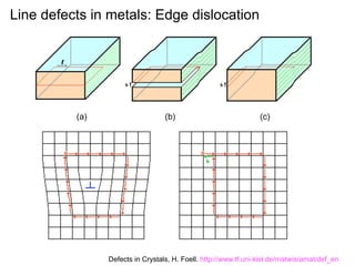
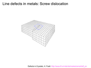
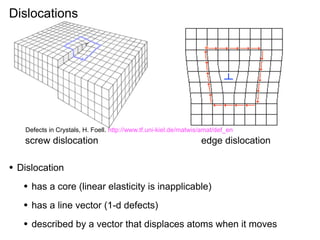
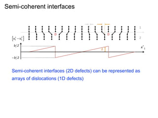
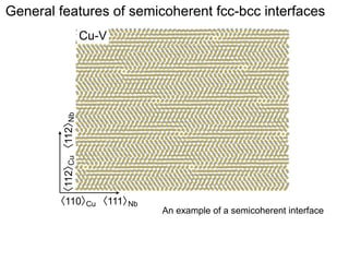
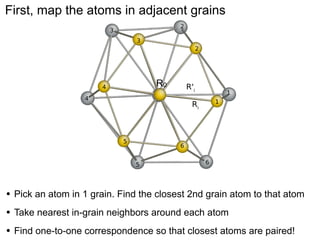
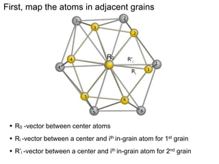
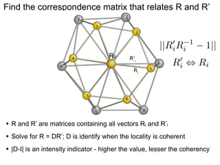
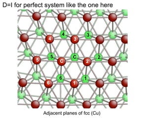
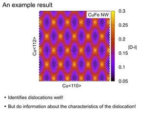
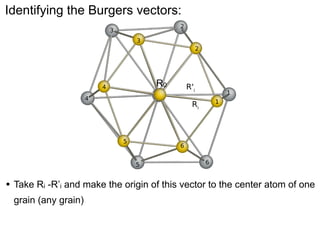
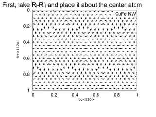
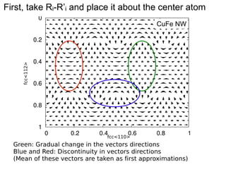
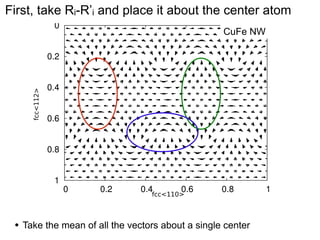
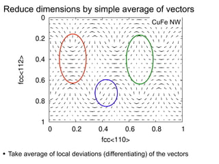
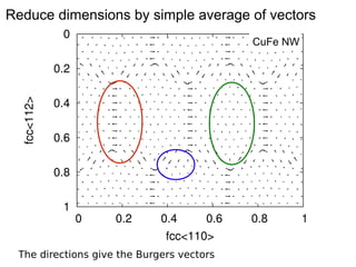
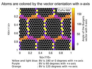
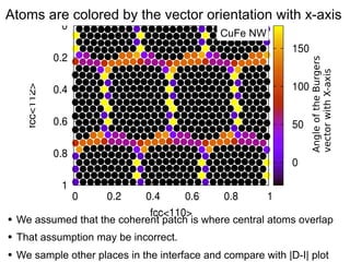
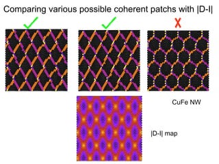
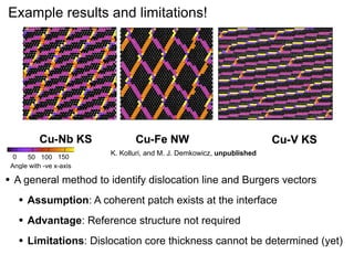
This document presents a new method for characterizing misfit dislocations at interfaces without requiring a reference structure. The method maps atoms in adjacent grains and computes vectors between closest atom pairs to identify coherent and incoherent regions. Taking the difference between these vectors approximates Burgers vectors of misfit dislocations. The method was demonstrated on a Cu-Fe nanowire interface, identifying multiple dislocation Burgers vectors that agreed with prior characterization. However, limitations include inability to determine dislocation core thickness.

1. Characterizing misfit dislocations at interfaces:
Yet Another Method!
Kedarnath Kolluri, M. J. Demkowicz
Acknowledgments:
A. Kashinath, A. Vattré, B. Uberuaga, X.-Y. Liu, A. Caro, and A. Misra
Financial Support:
Center for Materials at Irradiation and Mechanical Extremes (CMIME) at LANL,
an Energy Frontier Research Center (EFRC) funded by
U.S. Department of Energy, Office of Science, Office of Basic Energy Sciences

2. Classifying interfaces:
Coherent, semi-coherent, and incoherent boundaries
simplified side view
•
Lower and upper grains are in “perfect” alignment always

3. Classifying interfaces:
Coherent, semi-coherent, and incoherent boundaries
1
4
8
13
simplified side view
•
1
12
4
8
Lines of atoms are aligned perfectly only periodically

4. Coherent, semi-coherent, and incoherent boundaries
simplified side view
•
Atomic interactions generally reduce the “bad” patch
•
Coherent region experiences strain emanated by the “bad” patch
•
Interface with well separated “bad” patches may be described within
the same theory as that of dislocations: misfit dislocations
Semi-coherent interfaces (2D defects) can be represented as
arrays of dislocations (1D defects)

5. Line defects in metals: Edge dislocation
Defects in Crystals, H. Foell. http://www.tf.uni-kiel.de/matwis/amat/def_en

6. Line defects in metals: Screw dislocation
Defects in Crystals, H. Foell. http://www.tf.uni-kiel.de/matwis/amat/def_en

7. Dislocations
Defects in Crystals, H. Foell. http://www.tf.uni-kiel.de/matwis/amat/def_en
screw dislocation
•
edge dislocation
Dislocation
•
has a core (linear elasticity is inapplicable)
•
has a line vector (1-d defects)
•
described by a vector that displaces atoms when it moves

8. Semi-coherent interfaces
Semi-coherent interfaces (2D defects) can be represented as
arrays of dislocations (1D defects)

9. General features of semicoherent fcc-bcc interfaces
〈112〉 〈112〉
Cu
Nb
Cu-V
〈110〉 〈111〉
Cu
Nb
An example of a semicoherent interface

10. View of the Interface

11. View of the Interface

12. View of the Interface

13. View of the Interface

14. View of the Interface

15. View of the Interface

16. General features of semicoherent fcc-bcc interfaces
〈112〉 〈112〉
Cu
Nb
Cu-V
〈110〉 〈111〉
Cu
Nb
An example of a fcc-bcc semicoherent interface
Patterns corresponding to periodic “good” and “bad” regions

17. General features of semicoherent fcc-bcc interfaces
〈112〉 〈112〉
Cu
Nb
Cu-V
〈110〉 〈111〉
Cu
Nb
Interface contains arrays of misfit dislocations separating coherent
regions

18. 〈112〉 〈112〉
Cu
Nb
General features of semicoherent fcc-bcc interfaces
Cu-Nb
〈110〉 〈111〉
Cu
Nb
Cu-V
Interface contains arrays of misfit dislocations separating coherent
regions

19. MDI
1 nm
〈112〉
Cu
General features of semicoherent fcc-bcc interfaces
Cu-Nb KS 〈110〉
Cu
Cu-V KS
•
Two sets of misfit dislocations with Burgers vectors
•
Misfit dislocation intersections (MDI) where different sets of
dislocations meet

20. Sideviews often used to identify dislocation spacing
d = 2.55 nm
1
1
1
1
22
22
33
44
33
66
55
44
55
77
66
88
77
99
CuNb KS
10
10
88
99
<110>Cu || <111>Nb
<110>Cu || <111>Nb
In this case, dislocation spacing is 10 Cu interatomic plans (2.55 nm)
CuNb KS
d = 1.785 nm
11 22 33 4 4 5 5 6 6 7 7
11
22
33
44
55
66
<112>Cu || <112>Nb
<112>Cu || <112>Nb
In this case, dislocation spacing is 7 Cu interatomic plans (1.24 nm)

21. <112>Cu || <112>Nb
Side-views by themselves often tell wrong things!
2.1 nm
0.9 nm
<111>Cu ||
<110>Nb
<110>Cu || <111>Nb
•
12
Misfit dislocations in this case are not perpendicular to the sideview
•
The spacing obtained from sideview is not dislocation spacing!

22. Yet another method for finding dislocations
at fcc-bcc interfaces

23. First, map the atoms in adjacent grains
2
3
3
2
Cu-Fe NW
R0
4
R'i
4
1
1
Ri
5
6
5
6
Compute vectors R'i-Ri where the vectors are the lines joining
the closest
an atom in fcc and bcc atoms closest corresponding nearest
1 grain. Find the to their 2nd grain atom to that
neighbors
•
Pick
•
Take nearest in-grain neighbors around each atom
•
Find one-to-one correspondence so that closest atoms are paired!
atom

24. First, map the atoms in adjacent grains
2
3
3
2
Cu-Fe NW
R0
4
R'i
4
1
Ri
5
6
5
•
1
6
Compute vectors R'i-Ri where the
R0 -vector between center atoms vectors are the lines joining
•
the closest fcc and bcc atoms to their corresponding nearest
neighbors
Ri -vector between a center and ith in-grain atom for 1st grain
•
R’i -vector between a center and ith in-grain atom for 2nd grain

25. Find the correspondence matrix that relates R and R’
2
3
3
2
0
||Ri Ri
Cu-Fe NW
R0
4
R'i
4
1
Ri
5
0
Ri
1||
, Ri
6
5
•
1
1
6
Compute vectors containing all vectors Ri the R’i
R and R’ are matricesR'i-Ri where the vectors areand lines joining
•
the closest fcc and bcc atoms to their corresponding nearest
Solveneighbors
for R = DR’; D is identify when the locality is coherent
•
|D-I| is an intensity indicator - higher the value, lesser the coherency

26. D=I for perfect system like the one here
4
5
5
6
4
C
6
3
C
1
3
2
2
1
Adjacent planes of fcc (Cu)

27. An example result
NW
0.3
CuFe NW
0.25
0.4
Cu<112>
fcc<112>
0.35
0.3
0.2
0.55
0.1
0.6
0.05
0.45
Cu-Fe
|D-I|
0.15
0.5
Cu<110>
0.3 0.35 0.4 0.45 0.5 0.55 0.6
fcc<110>
•
Identifies dislocations well!
•
But do information about the characteristics of the dislocation!

28. Structure of interfaces: Misfit dislocations
•
A general method to identify dislocation line and Burgers vectors
•
Assumption: A coherent patch exists at the interface
•
Advantage: Reference structure not required
•
Limitations: Dislocation core thickness cannot be determined (yet)

29. Identifying the Burgers vectors:
2
3
3
2
Cu-Fe NW
R0
4
R'i
4
1
Ri
5
6
5
•
1
6
Compute vectors
Take Ri -R’i and makeR'i-Riorigin of this vector tothe lines joining of one
the where the vectors are the center atom
grain
the closest fcc and bcc atoms to their corresponding nearest
neighbors
(any grain)

30. First, take Ri-R’i and place it about the center atom
fcc<112>
CuFe NW
fcc<110>
The computed vectors are plotted. The vectors all originate at
the location of the center atom shown in slide 1

31. First, take Ri-R’i and place it about the center atom
fcc<112>
CuFe NW
fcc<110>
Green: Gradual change in the vectors directions
Blue and Red: Discontinuity in vectors directions
(Mean of these vectors are taken as first approximations)

32. First, take Ri-R’i and place it about the center atom
fcc<112>
CuFe NW
fcc<110>
Green: Gradual change in the vectors directions
Blue and Red: Discontinuity in vectors directions
Take of mean of all the vectors as first approximations)
•(Meanthe these vectors are takenabout a single center

33. Reduce dimensions by simple average of vectors
CuFe NW
•
Take average of local deviations (differentiating) of the vectors

34. Reduce dimensions by simple average of vectors
CuFe NW
The directions give the Burgers vectors

35. Atoms are colored by the vector orientation with x-axis
Angle of the Burgers
vector with X-axis
CuFe NW
Yellow and light blue: BV is 180 or 0 degrees with +x-axis
Purple
: BV is 60 degrees with +x-axis
Orange
: BV is 120 degrees with +x-axis

36. Atoms are colored by the vector orientation with x-axis
Angle of the Burgers
vector with X-axis
CuFe NW
•
•
•
We assumed that the coherent patch is where central atoms overlap
Yellow and light blue: BV is 180 or 0 degrees with +x-axis
Purple
: BV is 60
That assumption may be incorrect. degrees with +x-axis
Orange
: BV is 120 degrees with +x-axis
We sample other places in the interface and compare with |D-I| plot

37. Comparing various possible coherent patchs with |D-I|
NW
NW
.3
NW
0.3
150
0.35
0.4
100
45
.5
55
50
0.5
0.550
Cu-Fe
0.4
100
1
Cu-Fe
0.45
0.5
1
50
5
0.55 0
0
NW
0.6
0.6
0.3 0.35 0.4 0.45 0.5 0.55 0.6 0.3 0.35 0.4 0.45 0.5 0.55 0.6 0.30.3
0.35 0.4 0.45 0.5 0.55 0.6
0.3
fcc<110>
fcc<110>
fcc<110> NW
CuFe
0.35
fcc<112>
.6
0.45
0.35 150
fcc<112>
.4
fcc<112>
35
0.3
0.4
0.45
0.5
0.25
0.2
Cu-Fe
|D-I|
0.15
0.55
0.1
0.6
0.05
map

38. 0.4
.2
0.6
0.4
Example results and limitations!
0.8
0.6
1
0.8
150
0
0.45
0.4
0.35
0.3
0.25
0.2
0 0.5
0.2
100
0.4
0.8
1 0.15
0.6
50
0
1
0
0.2
0.4
0.6
0.8
1
0
0.2
0.4
0.6
0.8
1
0.28
0.26
150
0.24
0.22
0.2
100
0.18
0.16
50
0.14
0.12
0.1
0
0.08
0.06
0
50 100 150
Angle with -ve x-axis
0
0
0.2
0.4
1
0.6
A general method to identify dislocation line and Burgers vectors
0.8
•
Angle with -ve x axis
K. Kolluri, and M. J. Demkowicz, unpublished
•
Assumption: A coherent patch exists at the interface
•
Advantage: Reference structure not required
•
Limitations: Dislocation core thickness cannot be determined (yet)