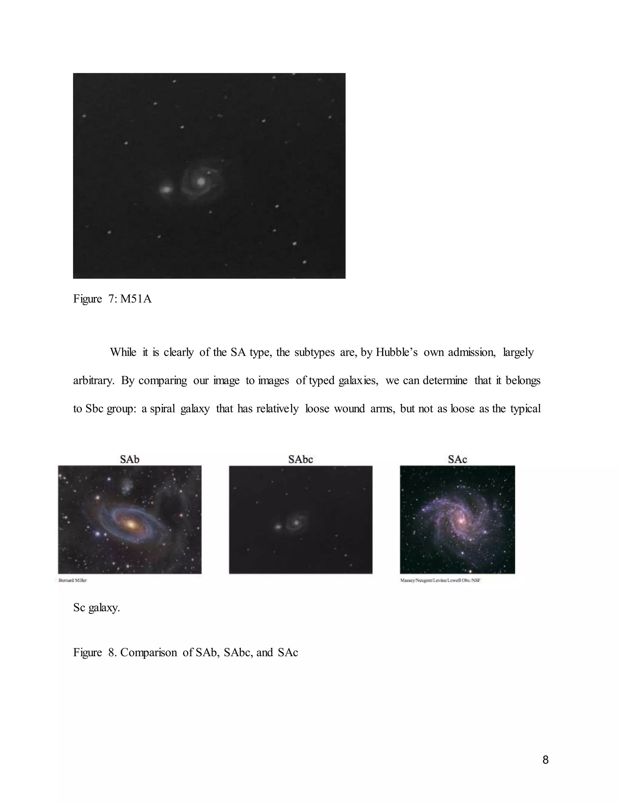
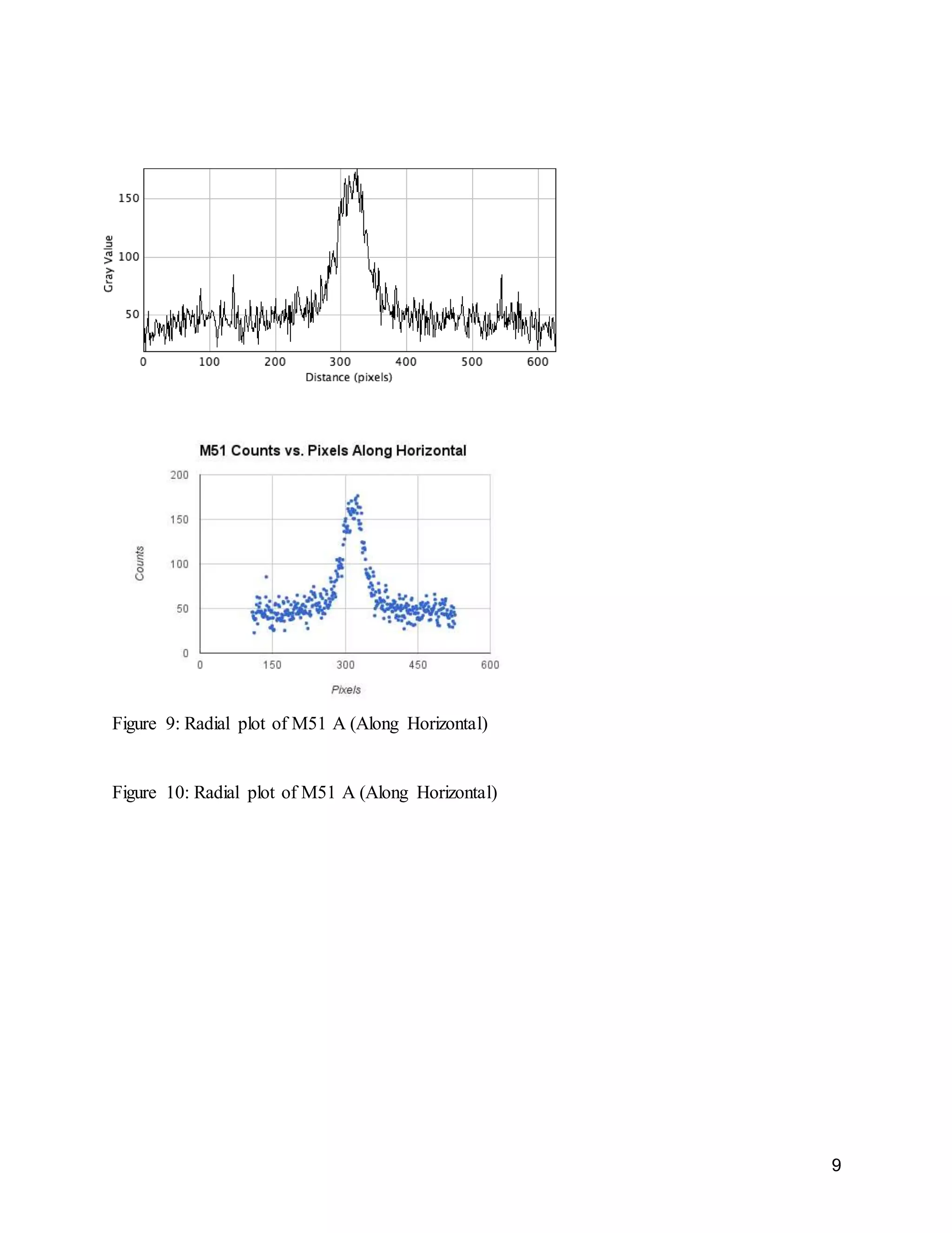
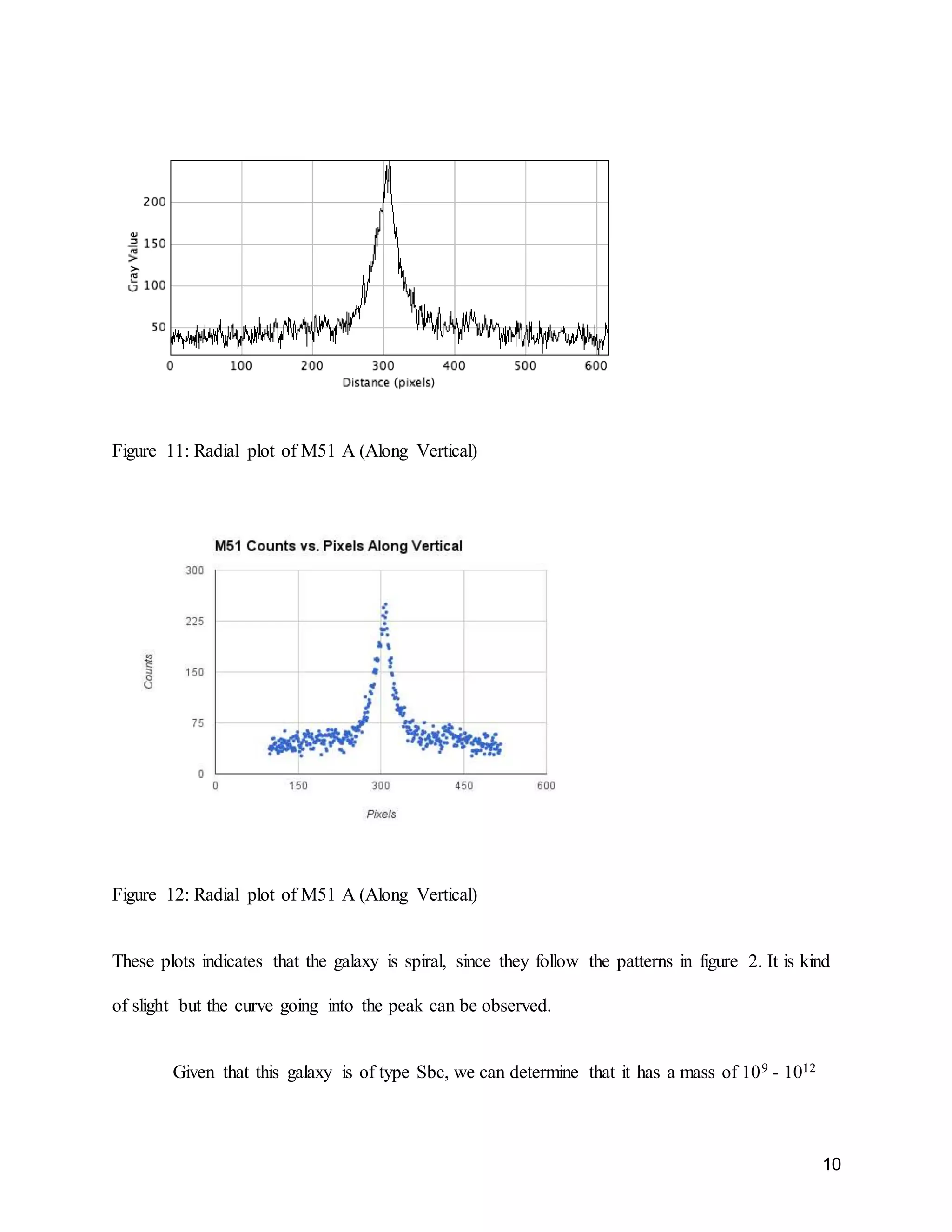
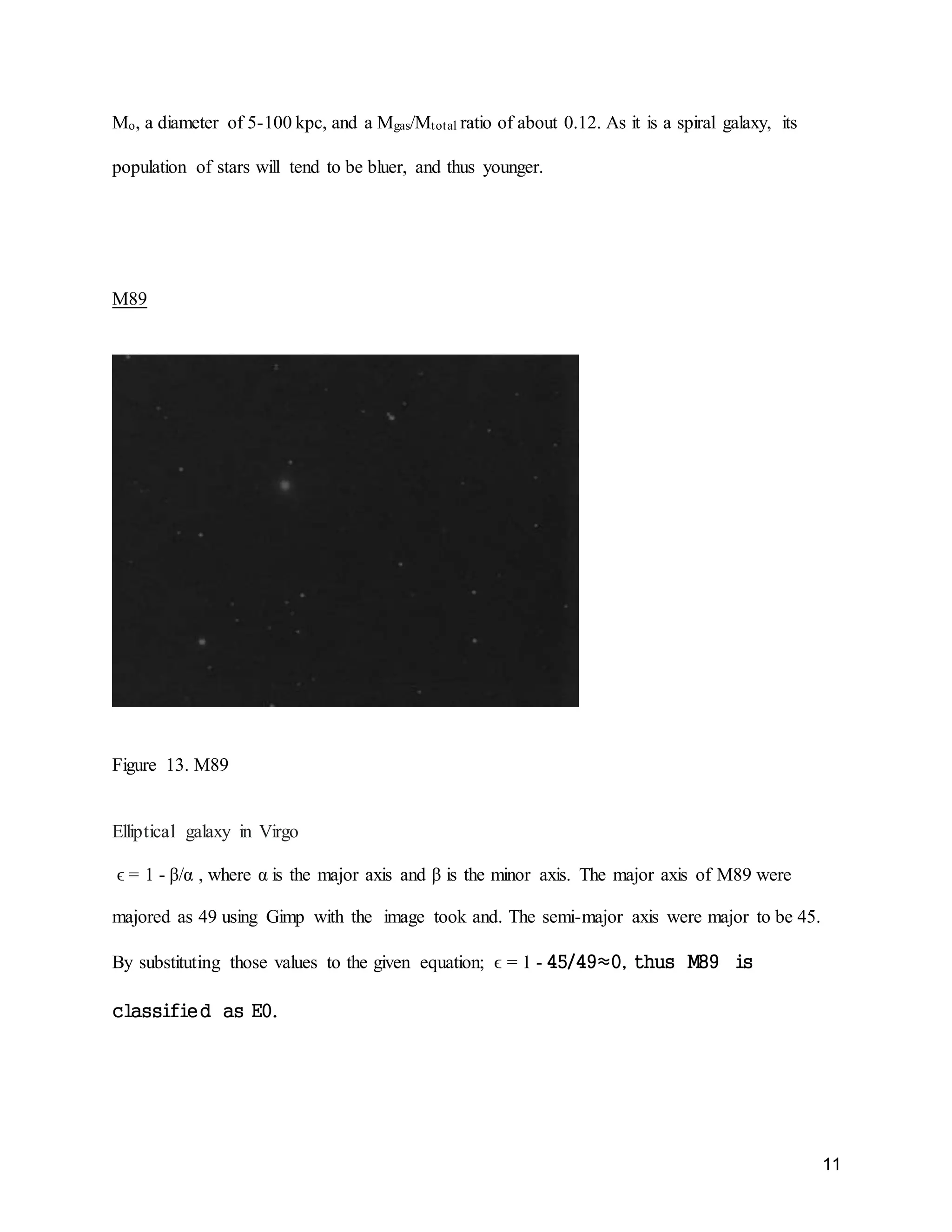
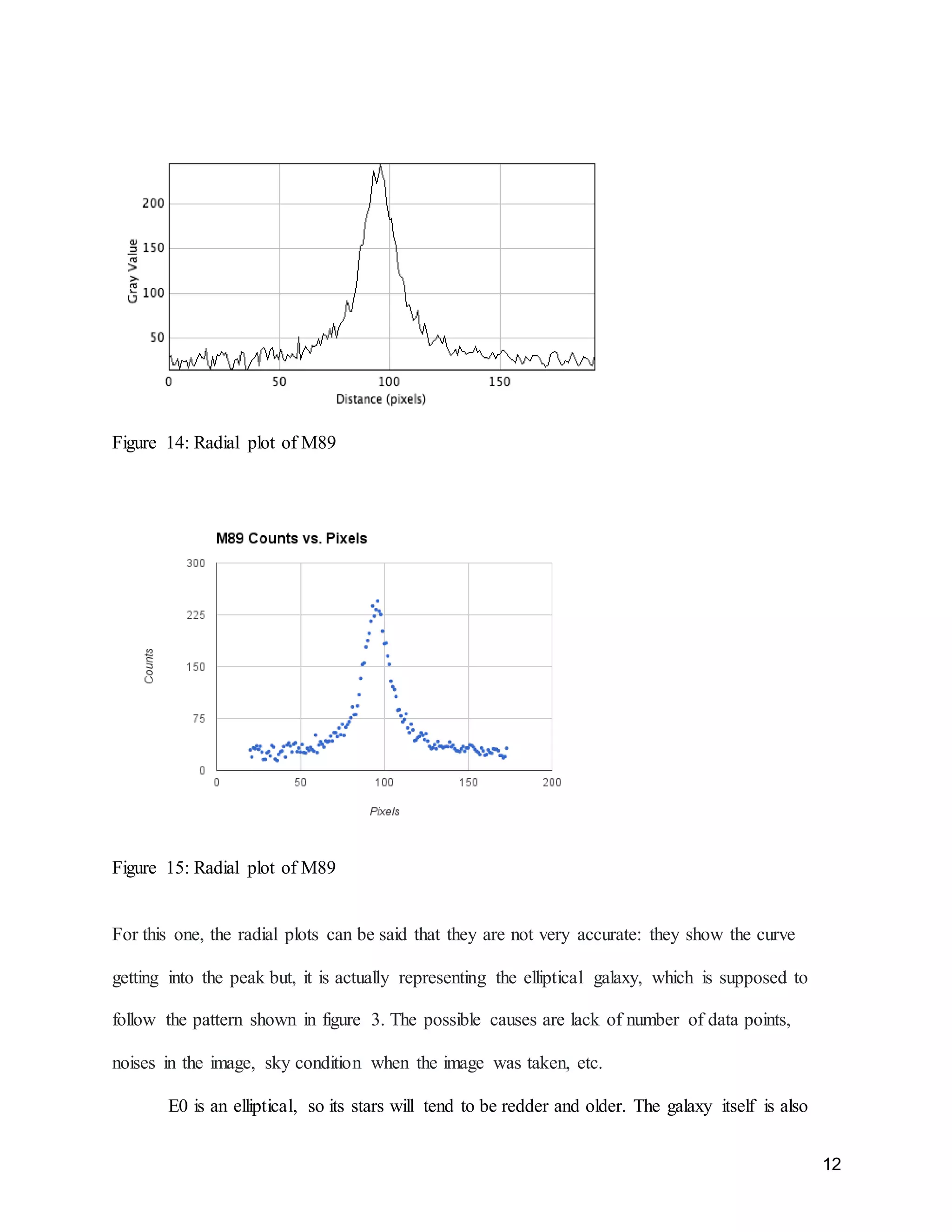
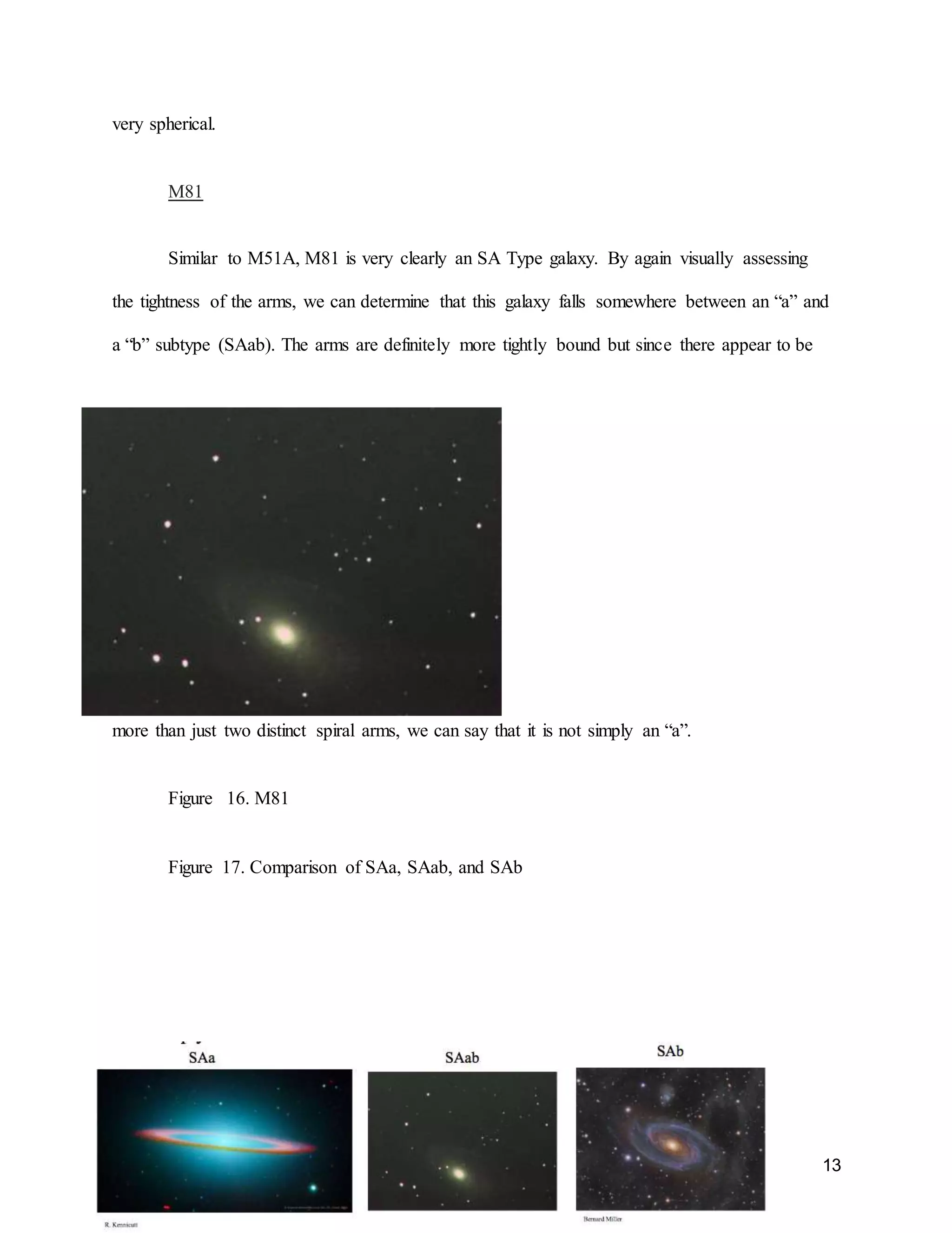
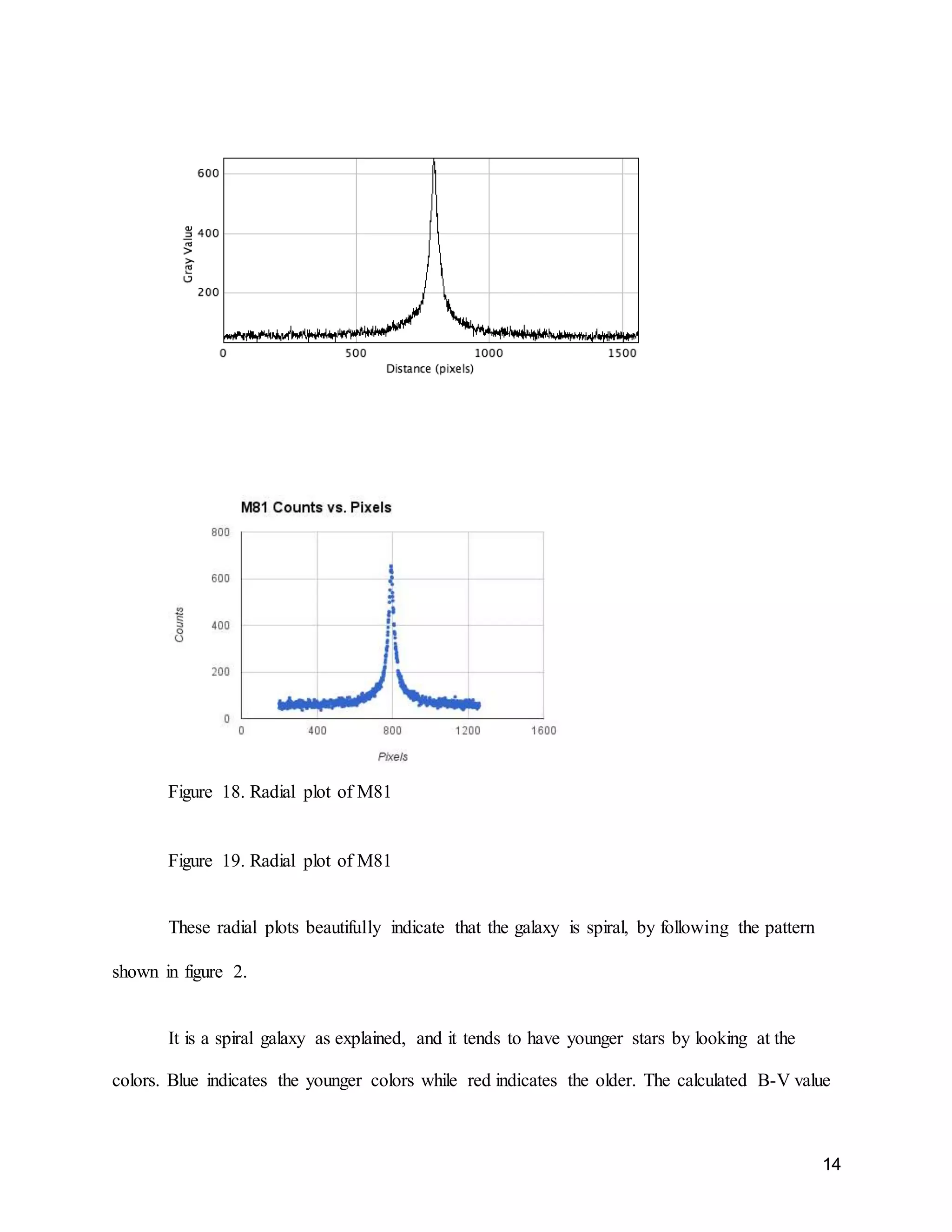
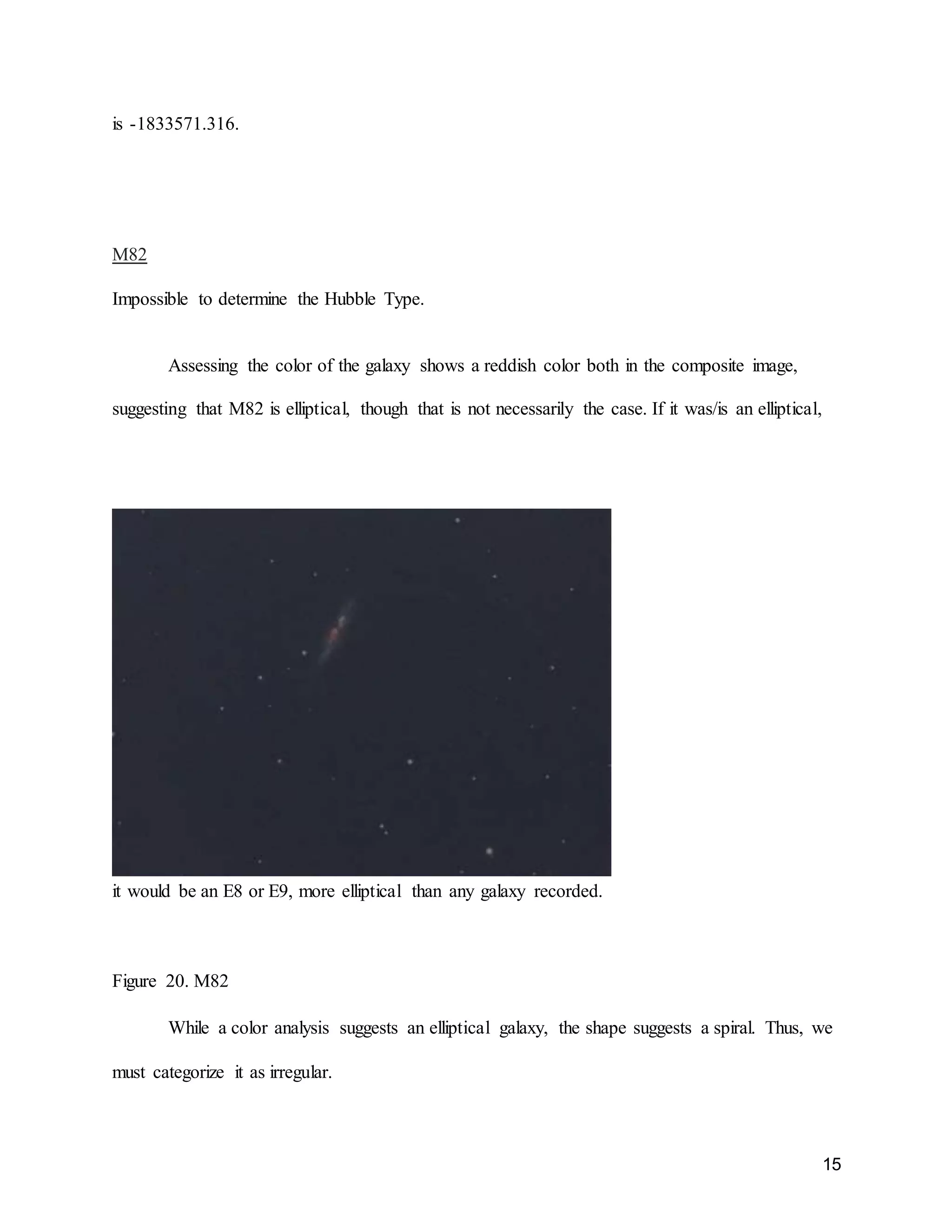
This document summarizes a student's observational astronomy project analyzing different galaxy types based on Hubble's Tuning Fork classification system. The student observed and analyzed images of 5 galaxies: NGC 4125 (E5 elliptical), M51 (Sbc spiral), M89 (E0 elliptical), M81 (SAab spiral), and M82. Ellipticity calculations classified the elliptical galaxies, while arm tightness classified the spirals. Radial plots also helped identify structure. The student found the galaxies matched their predicted Hubble types based on visual characteristics like color and shape.

1. PHYS 245
Observational Astronomy
Observational Project
5/29/16
Naomi Morishita
EXPLORING DIFFERENT TYPES OF GALAXIES
Abstract
This paper is going to address the theme “Exploring Different Galaxy Types”. In this
paper, the “exploration” is particularly based on Hubble Tuning Fork, the classification of
galaxies that an American astronomer, Edwin Hubble established in 1926. This theme is
interesting because Hubble Tuning Fork presents a method for statistically classifying galaxies,
from which quantitative assessments can be made. Also, it can be used to make statements such
as “The percent of galaxies in this area is x” or “This type of galaxy is more commonly observed

2. 1
than that type”. Hubble stated that “The classification was devised primarily for statistical
studies” in his paper, but still, a number of physical characteristics can be derived from
determining the Hubble Type. My group analyzed five galaxies in the aspects of their sizes, color
and shape by looking at the image, calculating the ellipticity and also the grey value plots (radial
plots). The data analysis and its process of the each galaxy and their significance will be
discussed in the following sections.
Introduction

3. 2
Hubble Tuning Fork was established by American astronomer Edwin Hubble 1926. It
classifies the galaxies mainly by on their visual appearance or morphologies. The biggest two
categories of the galaxies are elliptical and spiral. The types of elliptical galaxies are classified
with subgroups from E0 to E7, with E0 group being most round and E7 being most elliptical.
The specific group a galaxy belongs are determined by the mathematical equation based on its
major and minor axis, which going to be introduced in the following sections. The spiral galaxies
are first classified as either spiral galaxy or barred spiral galaxy. In both groups, the galaxies are
classified into subgroups depending on how tight their wounds are. “S” represents the spiral
galaxy group and “SB” represents the barred spiral galaxy group. In those two groups, there are
galaxies belonging to subgroups ranging from S(B)a to S(B)c, as shown in Figure 1 below.
Galaxies on the left are termed “early”, ones on the right are “late” and galaxies in the middle are
“intermediate” . Opposing to our intuition, this terminology does not refer to the age of the
galaxies, as Hubble Stated in his paper, “The nomenclature, it is emphasized, refers to position in
the sequence and temporal connotations are made at one's peril.”

4. 3
Figure 1. Hubble Tuning Fork
Hubble Tuning Fork is still used by many researchers today. As its current status, NASA
had a project in 2013 that they made a comparison between the galaxy images that Hubble had
taken and the current images of those galaxies. They found out that even though the size of the
galaxies are growing, the basic pattern of the galaxy structures had not changed since 11 billion
years ago. In this paper, specifically the images of NGC 4125 (E5) , M51 “Whirlpool Galaxy”
(Sbc), M89(E0), M81 (Sab), and M82(E8/E9) will be discussed. These images, except M82
have been taken with R, V, and B filters by us. Then they were reduced and stacked using
Dawn, and three color images were produced by using Gimp for those that we were able to.
Since classifications were originally based on their visual appearance or morphologies, this paper
is analyzing the five galaxies by their groups they belong in Hubble Tuning Fork, and their
“roundness”,wounds, and other apparel aspects. Then we see how well the the images of galaxies
we took and analyzed are fitting the group they actually belong to. Also, for the elliptical
galaxies, major and minor axes have been majored to determine the Hubble Type from the image
we have taken. In addition to that, using Astroimage J, Gray values (counts) vs. Pixels plots
(radial plots) are created for the galaxies NGC 4125, M51, M89, and M81. The grey values
(counts) represents how bright the particular spot in the image is. The lower the grey value, the
dimmer the spot is and vise versa. By looking at the plots, we are able to determine the galaxy
shapes: if there is a curve from the background sky to the galaxy on the plot, we analyze it as a
spiral galaxy, since it indicates the disk (See figure 2 below). If there is no curve from the
background sky to going up to the peak (center of the galaxy), we analyze it as an elliptical
galaxy (See figure 3 below). The detailed procedure and their analysis will be discussed in the
following section.

5. 4
Figure 2. Expected plot type of radial plot of spiral galaxies
Figure 3. Expected plot type of radial plot of elliptical galaxies
Data Acquisition:
During the observation process, me and my group spend few nights to take the images of
relatively luminous and “face-on” galaxies with different characteristics. We used the cycle
exposure function and took plenty of images that are exposed for 30 seconds, 60 seconds, and 90
seconds. Due to the weather and sky conditions, we were not able to get as many images as we
wanted at the quality we had expected, by at least we got enough to analyze, and we also used
the images that were not taken by us.

6. 5
Since Hubble Types are mainly about the appearance of the galaxies, we were
able to learn a lot from the images, though the further quantitative analysis gave us much more
information as we kept on analyzing. Followings are the quantitative methods that were used to
analyze the galaxies.
For the elliptical galaxies, we used the equation ϵ = 1 - β/α , to classify the subgroups that
a galaxy would belong, where α is the major axis and β is the minor axis. For example, the major
axis of NGC 4125 were majored as 77 using Gimp with the image we took and. The semi-major
axis were major to be 40. By substituting those values to the given equation; ϵ = 1 - 40/77≈0.5,
thus NGC 4125 is classified as E5. For M89 has been calculated the
same way. For the spiral galaxies, the comparison with the group
previous and following the group a galaxy belongs are done and also
the plots of grey values (counts) vs. pixels, are presented. We also
analyzed some of them by focusing on their color (B-V value) and the
radial function.
Results/Discussion:
NGC 4125:
Elliptical galaxy in Draco

7. 6
Figure 4: NGC 4125
ϵ = 1 - β/α , where α is the major axis and β is the minor axis. The major axis of NGC
4125 were majored as 77 using the image took and Gimp. The semi-major axis were major to be
40. By substituting those values to the given equation; ϵ = 1 - 40/77≈0.5, thus NGC 4125
is classified as E5.
It belongs to E5 group in Hubble Tuning Fork, which is an elliptical galaxy that is
relatively close to S0 group (lenticular). As it is an elliptical galaxy, its population of stars will
tend to be redder, and thus older by the B-V value -47495.91029.

8. 7
Figure 5: Radial plot of NGC 4125
Figure 6: Radial plot of NGC 4125
These radial plots are fluctuating a lot, but it indicates that the galaxy is elliptical since it is
following the pattern shown in figure 3.
M51 A
Spiral galaxy in Canes Venatici, also known as the “Whirlpool Galaxy”. The other object is
M51B

9. 8
Figure 7: M51A
While it is clearly of the SA type, the subtypes are, by Hubble’s own admission, largely
arbitrary. By comparing our image to images of typed galaxies, we can determine that it belongs
to Sbc group: a spiral galaxy that has relatively loose wound arms, but not as loose as the typical
Sc galaxy.
Figure 8. Comparison of SAb, SAbc, and SAc

10. 9
Figure 9: Radial plot of M51 A (Along Horizontal)
Figure 10: Radial plot of M51 A (Along Horizontal)

11. 10
Figure 11: Radial plot of M51 A (Along Vertical)
Figure 12: Radial plot of M51 A (Along Vertical)
These plots indicates that the galaxy is spiral, since they follow the patterns in figure 2. It is kind
of slight but the curve going into the peak can be observed.
Given that this galaxy is of type Sbc, we can determine that it has a mass of 109 - 1012

12. 11
Mo, a diameter of 5-100 kpc, and a Mgas/Mtotal ratio of about 0.12. As it is a spiral galaxy, its
population of stars will tend to be bluer, and thus younger.
M89
Figure 13. M89
Elliptical galaxy in Virgo
ϵ = 1 - β/α , where α is the major axis and β is the minor axis. The major axis of M89 were
majored as 49 using Gimp with the image took and. The semi-major axis were major to be 45.
By substituting those values to the given equation; ϵ = 1 - 45/49≈0, thus M89 is
classified as E0.

13. 12
Figure 14: Radial plot of M89
Figure 15: Radial plot of M89
For this one, the radial plots can be said that they are not very accurate: they show the curve
getting into the peak but, it is actually representing the elliptical galaxy, which is supposed to
follow the pattern shown in figure 3. The possible causes are lack of number of data points,
noises in the image, sky condition when the image was taken, etc.
E0 is an elliptical, so its stars will tend to be redder and older. The galaxy itself is also

14. 13
very spherical.
M81
Similar to M51A, M81 is very clearly an SA Type galaxy. By again visually assessing
the tightness of the arms, we can determine that this galaxy falls somewhere between an “a” and
a “b” subtype (SAab). The arms are definitely more tightly bound but since there appear to be
more than just two distinct spiral arms, we can say that it is not simply an “a”.
Figure 16. M81
Figure 17. Comparison of SAa, SAab, and SAb

15. 14
Figure 18. Radial plot of M81
Figure 19. Radial plot of M81
These radial plots beautifully indicate that the galaxy is spiral, by following the pattern
shown in figure 2.
It is a spiral galaxy as explained, and it tends to have younger stars by looking at the
colors. Blue indicates the younger colors while red indicates the older. The calculated B-V value

16. 15
is -1833571.316.
M82
Impossible to determine the Hubble Type.
Assessing the color of the galaxy shows a reddish color both in the composite image,
suggesting that M82 is elliptical, though that is not necessarily the case. If it was/is an elliptical,
it would be an E8 or E9, more elliptical than any galaxy recorded.
Figure 20. M82
While a color analysis suggests an elliptical galaxy, the shape suggests a spiral. Thus, we
must categorize it as irregular.

17. 16
As this paper has been addressing, the Hubble Tuning Fork is a very useful to classify the
galaxies in many different aspects. However, there are some limitations of it. Hubble Tuning
Fork fails to provide classification for irregular galaxies beyond lumping them into the categories
Irr I and Irr II. Also, it may lead to a misconception that the galaxies evolve from E0 group to
either Sc or SBc group, by calling the ones on the left “early” ones and the ones on the right
“late” ones even though that was just Hubble states on his paper “It is just an arbitrary procedure
and is adopted merely because it is possible to distinguish the middle section from the two ends”.
Summary
Using the images that we have taken, we calculated ϵ values for the elliptical galaxies
and compared to the actual groups that those galaxies belong to. For the spiral galaxies we made
comparisons with the galaxies in nearby subgroups by their tightness in the wounds. Then, for
both of them,we compared the observed color and grey value functions and compared. We then
made comments on each comparisons and the things we were able to learn about the galaxies
other than determining their Hubble Types.
It is significant that we keep exploring different types of galaxies even though Hubble
had made the “standard classification”, because there are many aspects in galaxy
formation/evolution that have not yet been discovered. Exploring the different types of galaxies
over long time periods gives us significant amount of information that we can use to test our

18. 17
predictions.
For the future reference, we would start observing earlier so that we get enough/back up
nights for observation. Also for the further analysis, we would take the uncertainties to account.
References
Longair, M. S. Galaxy Formation. Berlin: Springer, 2008. Print.
Takamori, Keisuke. Uchu Ni Tsuite Shiritai Rokujuhachikomoku: Hoshizora to Uchu Ga Attoteki
Ni Omoshiroku Naru. N.p.: Newton, n.d. Print.

19. 18
Carroll, Bradley W., and Dale A. Ostlie. An Introduction to Modern Astrophysics. San Francisco,
Calif. ; Munich: Pearson/Addison Wesley, 2009. Print.
"1971JHA.....2..109H Page 109." 1971JHA.....2..109H Page 109. N.p., n.d. Web. 31 May 2016.
※All of the image citations on the images.