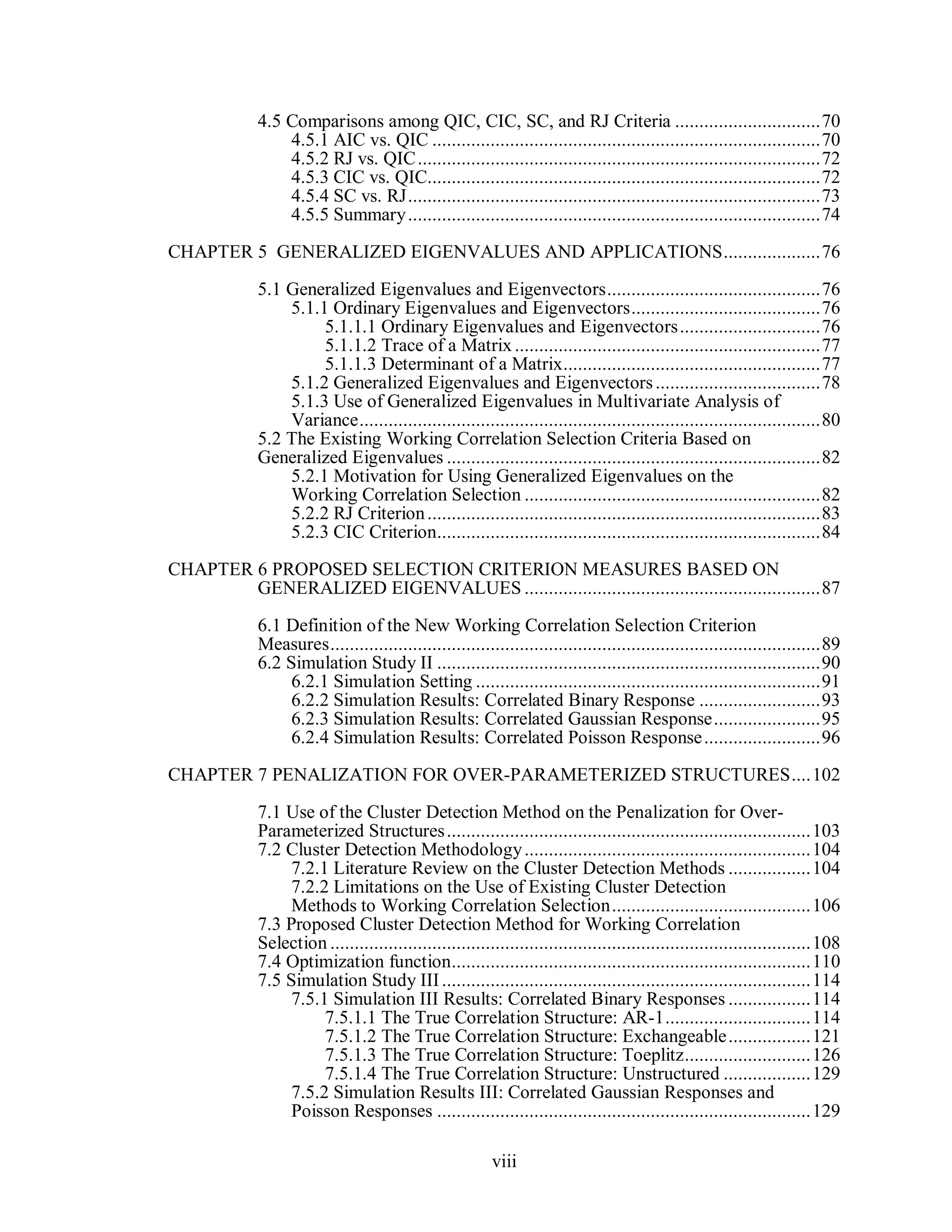
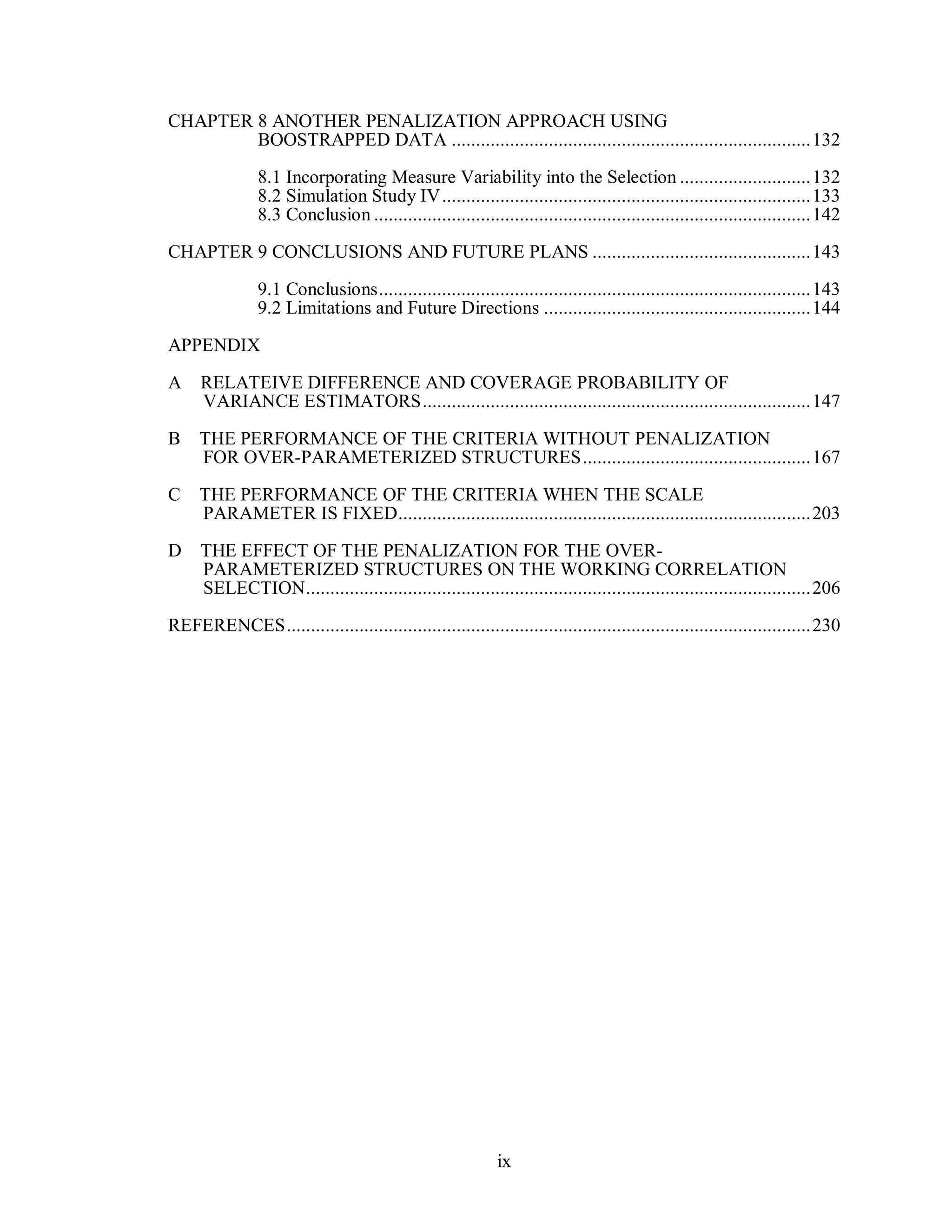
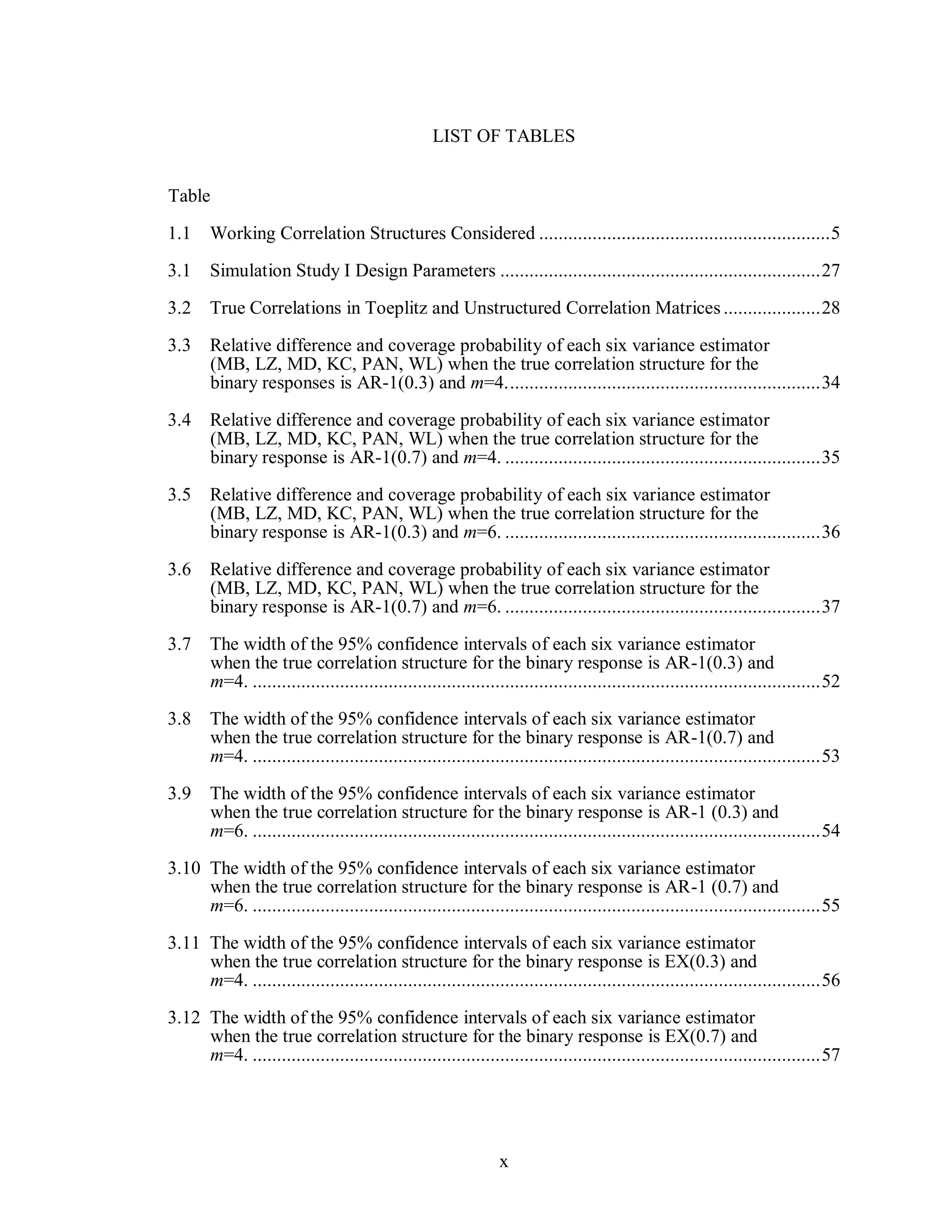
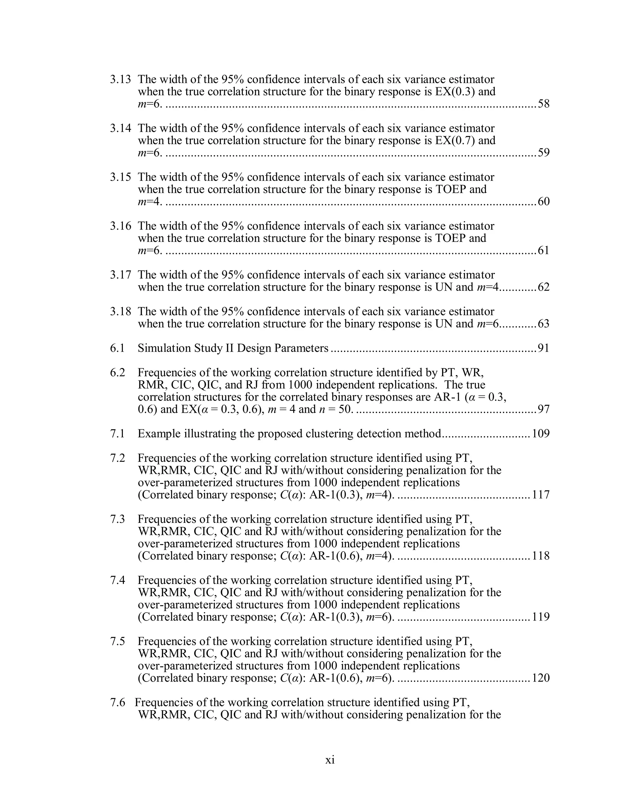
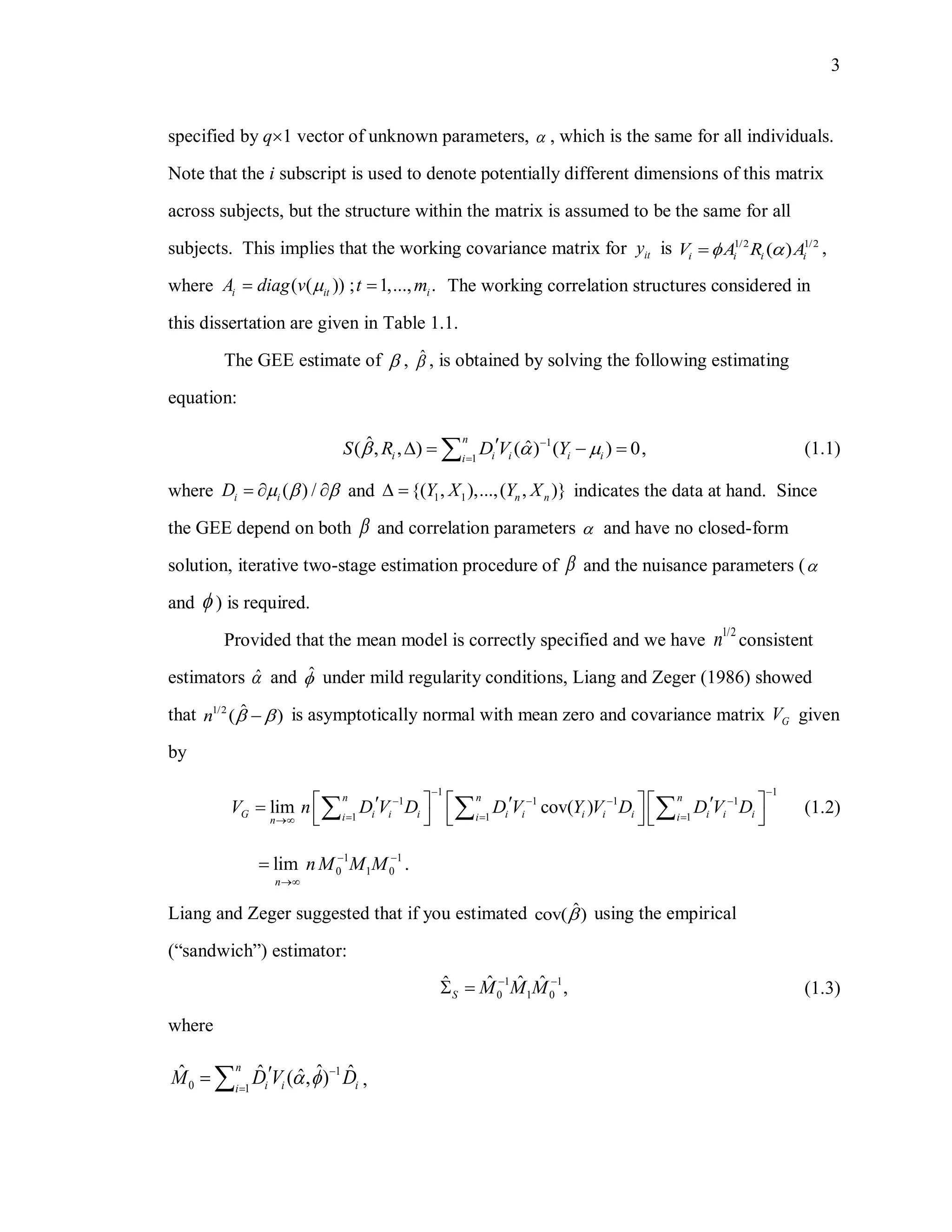
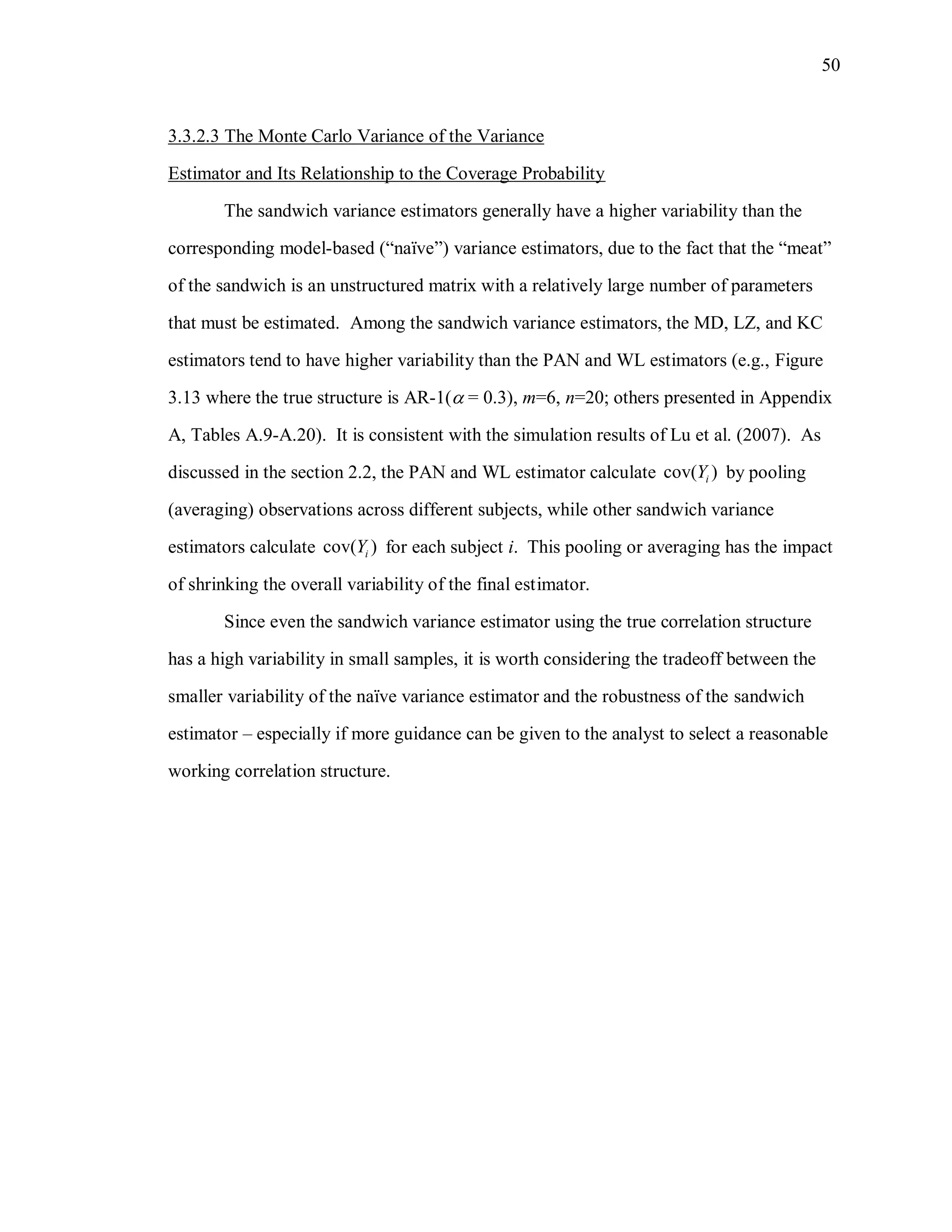
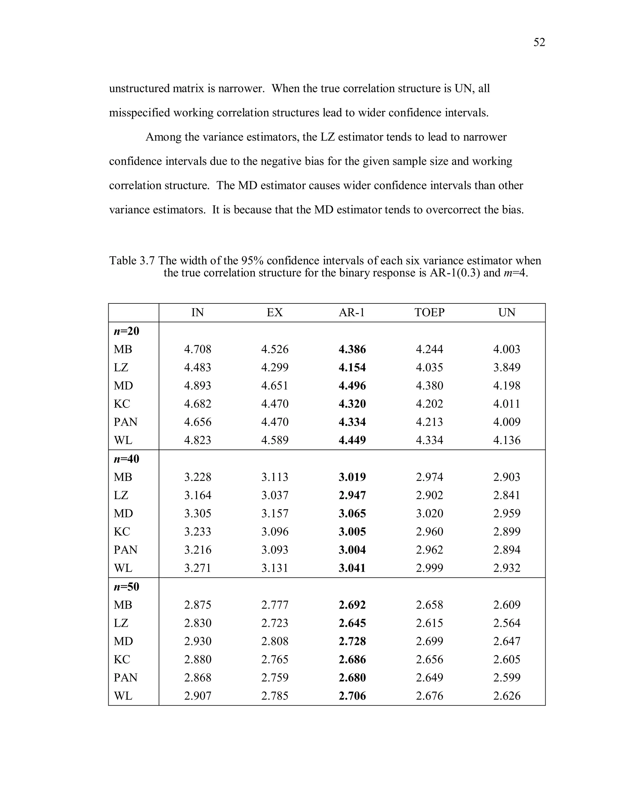
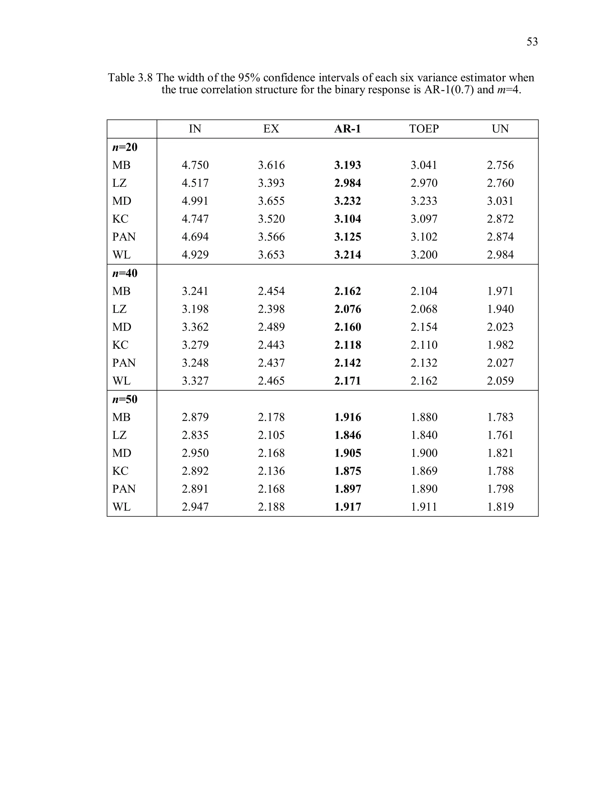
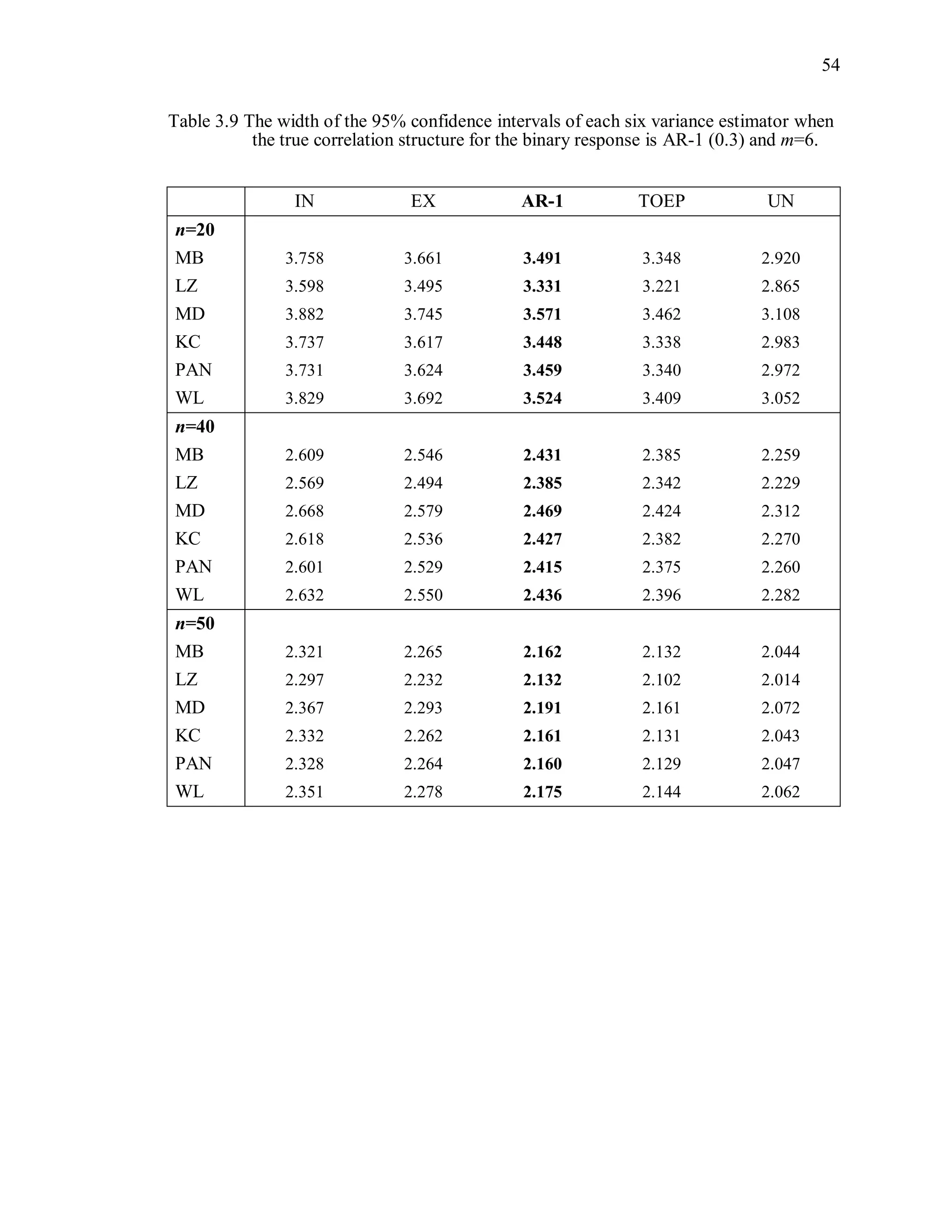
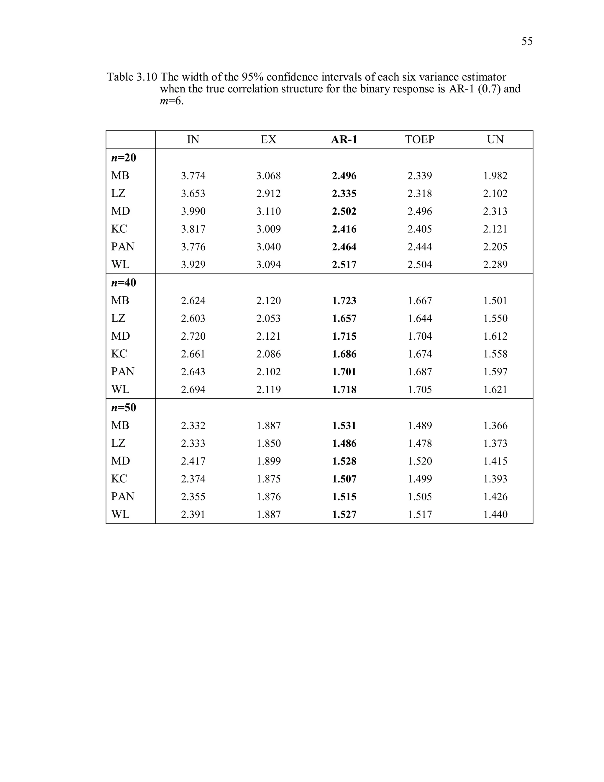
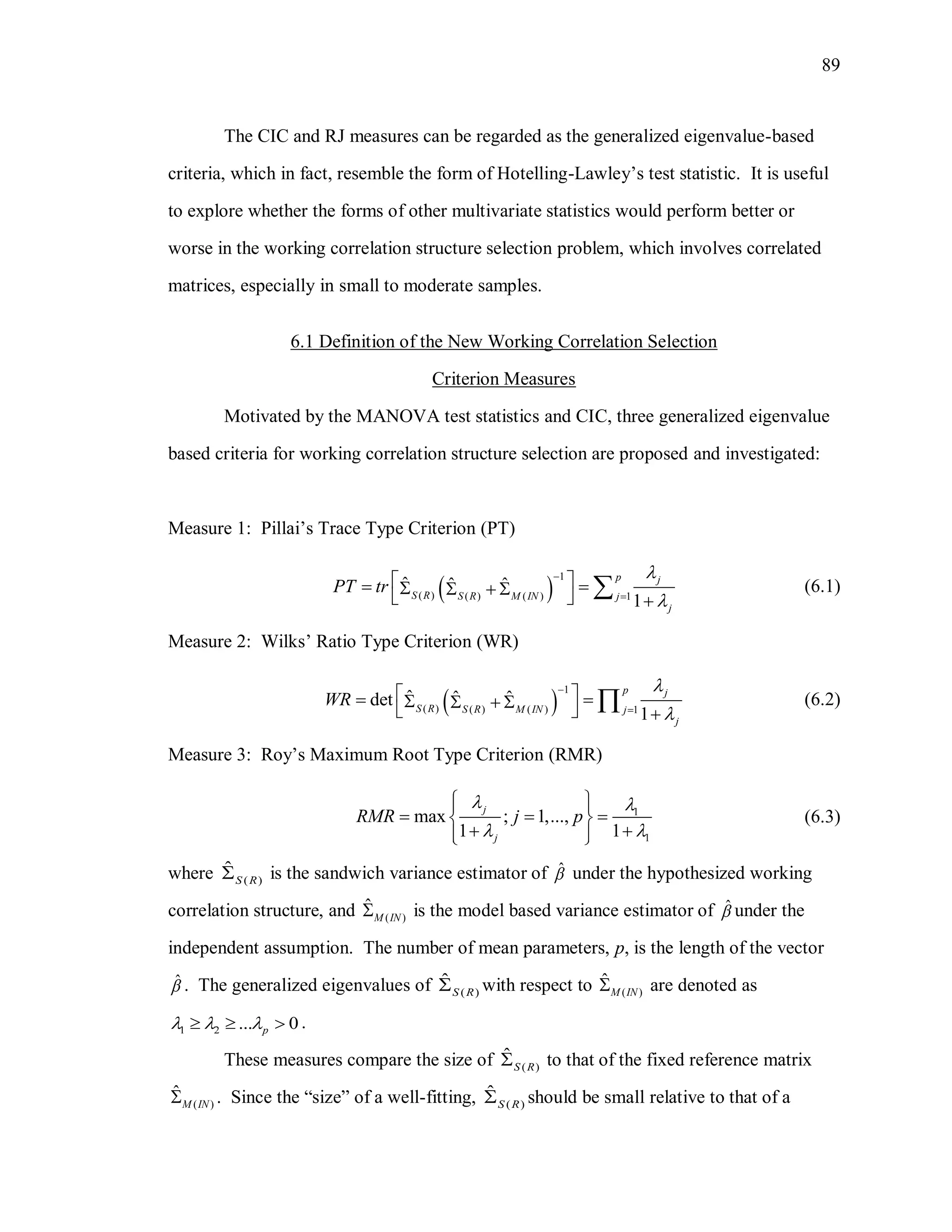
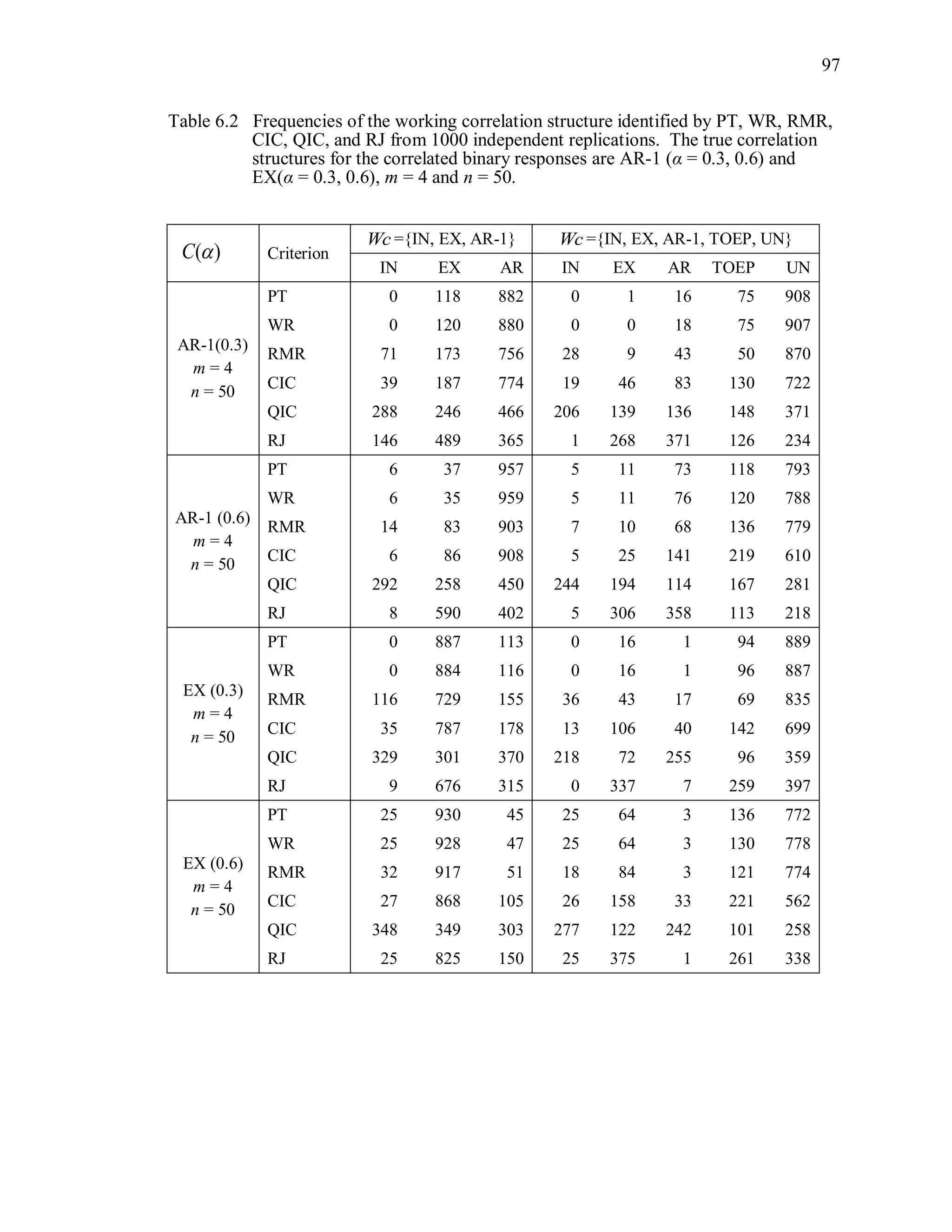
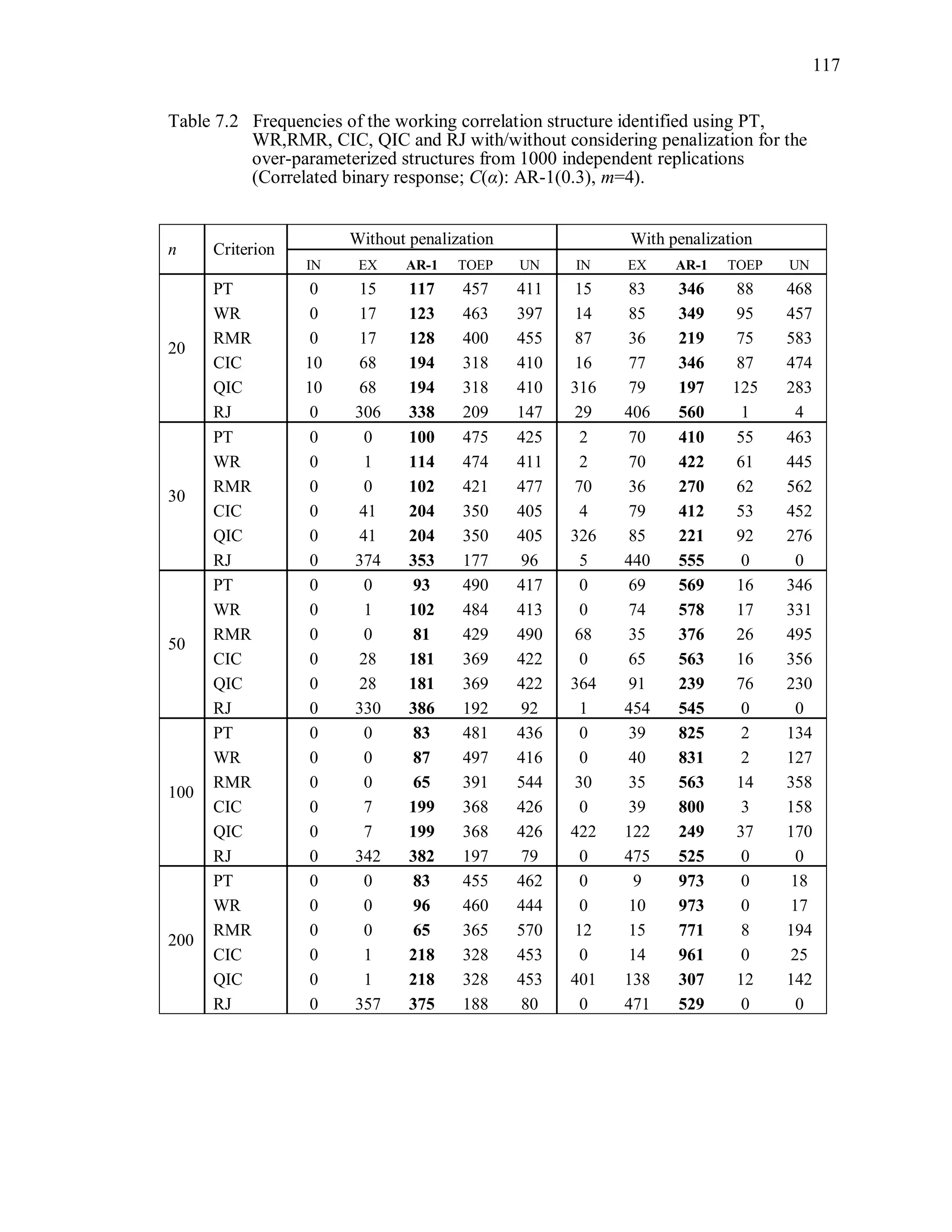
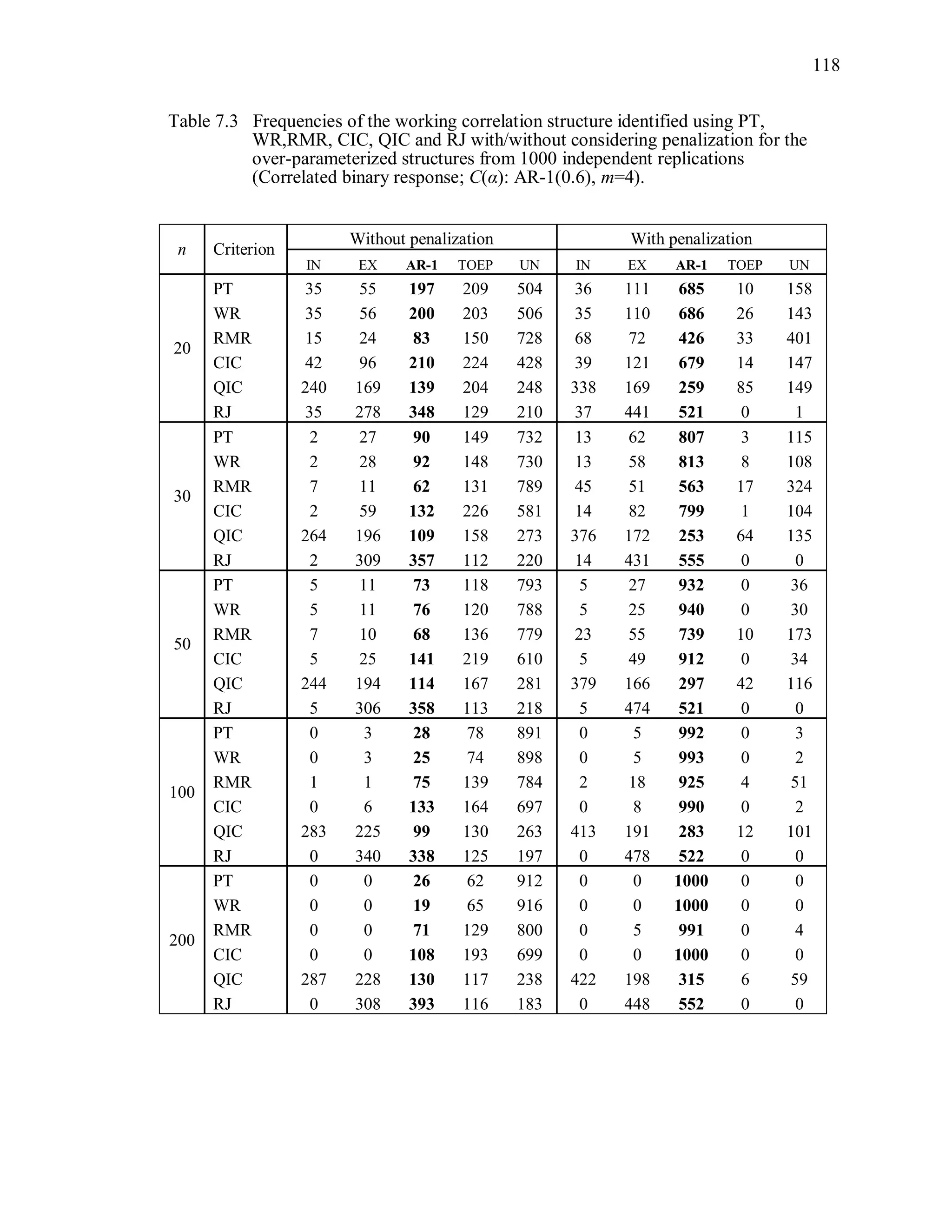
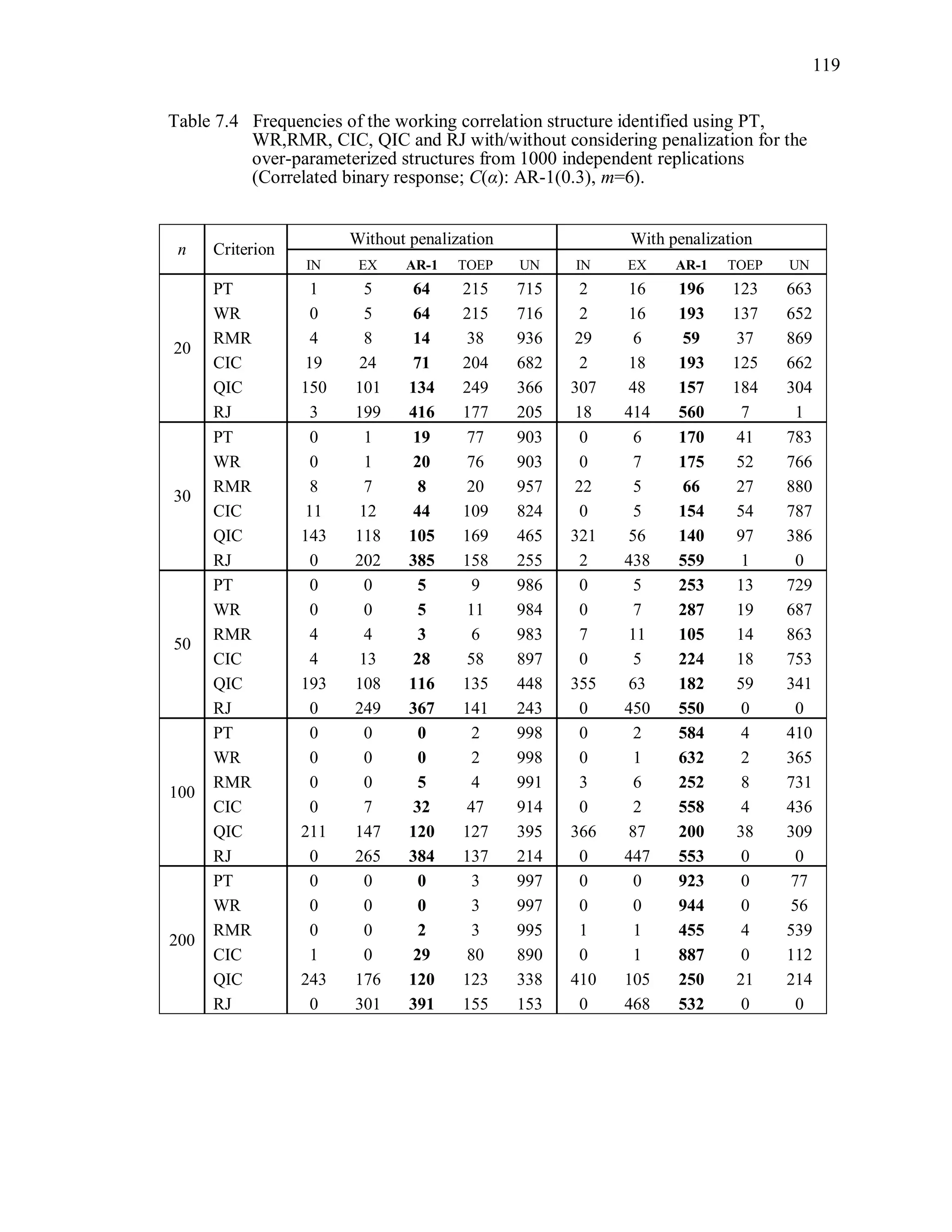
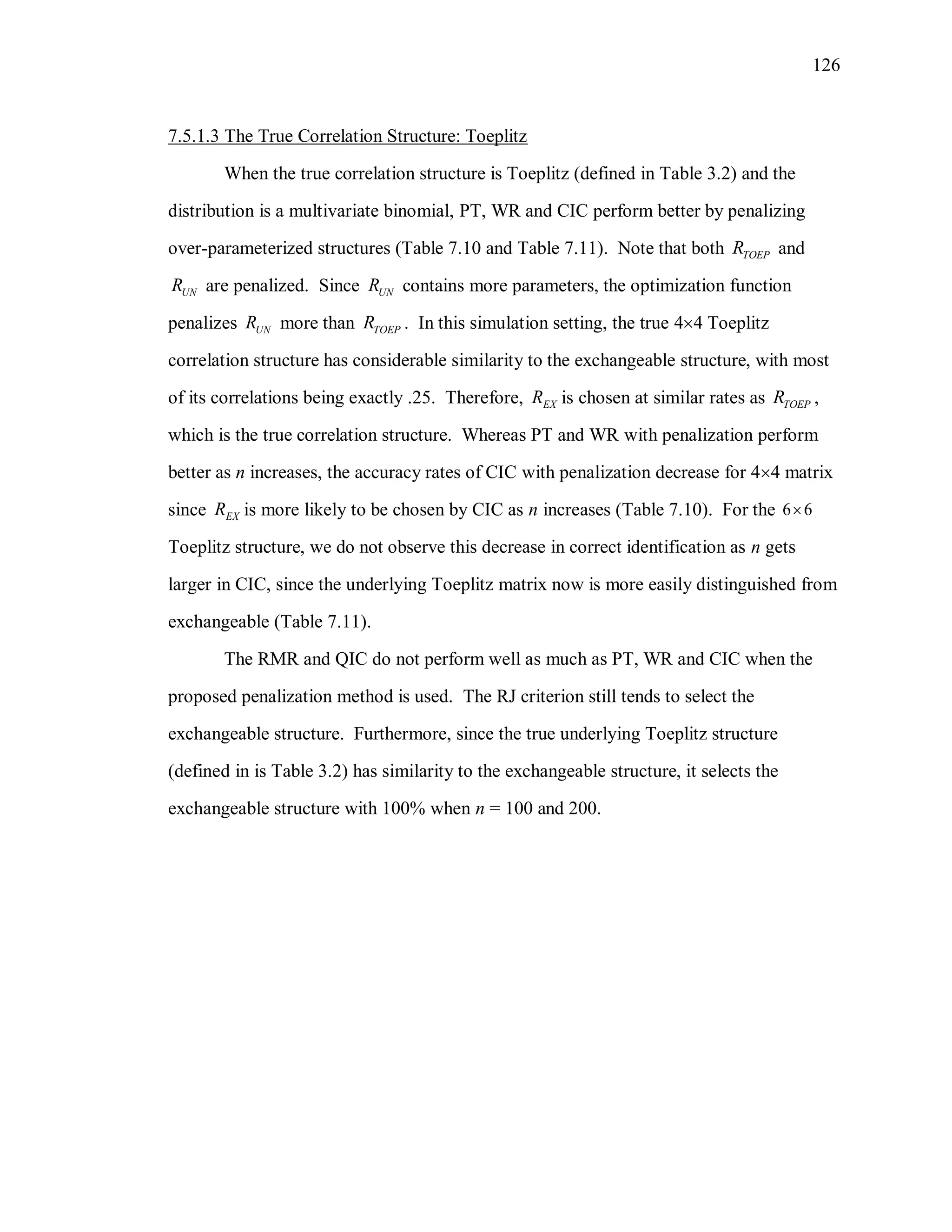
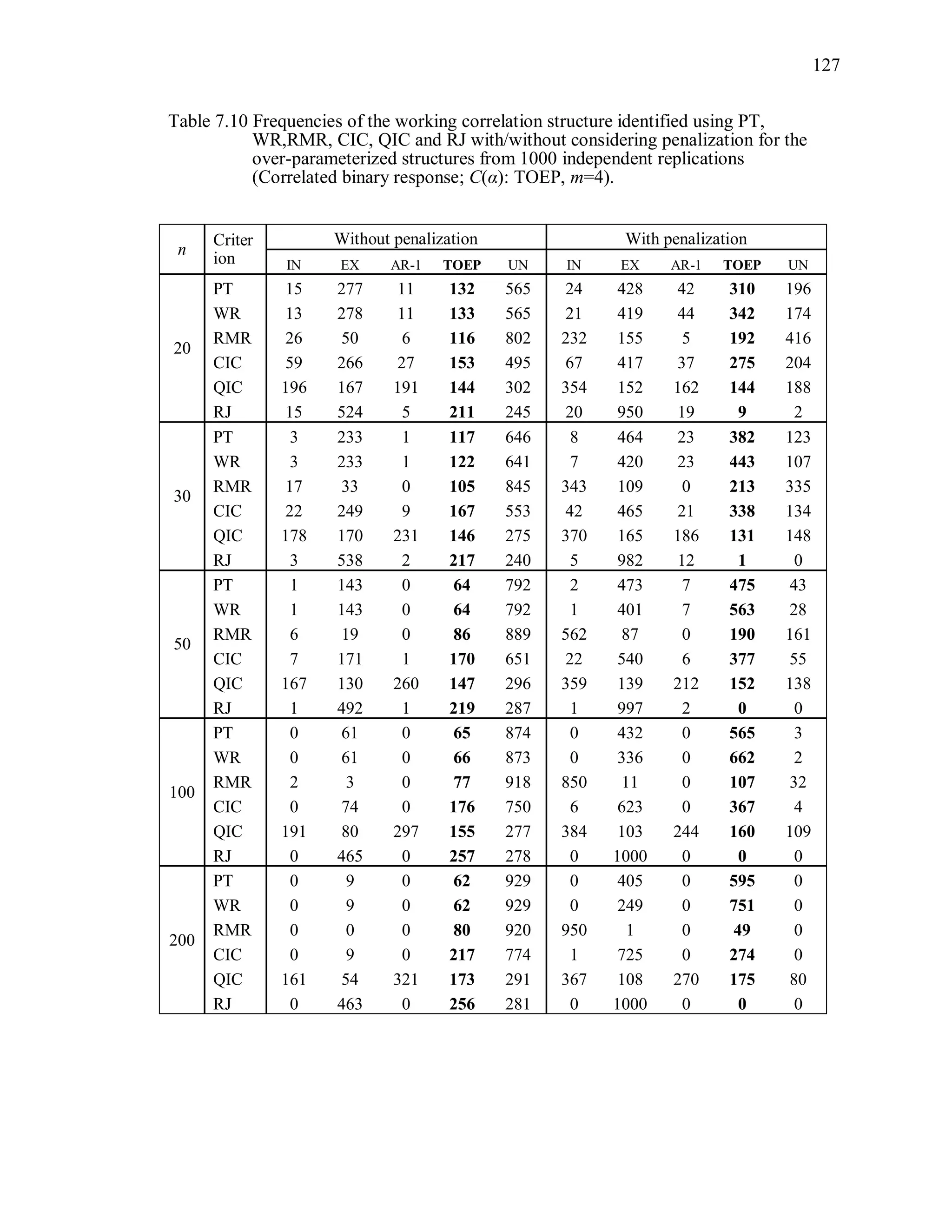
This document summarizes Mi Jin Jang's dissertation which develops new criteria for selecting the working correlation structure in generalized estimating equations (GEE) models. The dissertation proposes using generalized eigenvalues to measure the disparity between variance estimators under different working correlation structures. Three new selection criteria are developed based on generalized eigenvalues: Pillai's trace (PT) criterion, Wilks' ratio (WR) criterion, and Roy's maximum root (RMR) criterion. The dissertation also develops methods to penalize over-parameterized working correlation structures which may be favored by existing criteria. Simulation studies demonstrate the performance of the proposed criteria.

1. Masthead Logo
University of Iowa
Iowa Research Online
Theses and Dissertations
Fall 2011
Working correlation selection in generalized
estimating equations
Mi Jin Jang
University of Iowa
Copyright 2011 Mijin Jang
This dissertation is available at Iowa Research Online: https://ir.uiowa.edu/etd/2719
Follow this and additional works at: https://ir.uiowa.edu/etd
Part of the Biostatistics Commons
Recommended Citation
Jang, Mi Jin. "Working correlation selection in generalized estimating equations." PhD (Doctor of Philosophy) thesis, University of
Iowa, 2011.
https://doi.org/10.17077/etd.kj4igo6k

2. WORKING CORRELATION SELECTION IN GENERALIZED ESTIMATING
EQUATIONS
by
Mi Jin Jang
An Abstract
Of a thesis submitted in partial fulfillment
of the requirements for the Doctor of
Philosophy degree in Biostatistics
in the Graduate College of
The University of Iowa
December 2011
Thesis Supervisor: Professor Jane F. Pendergast

3. 1
ABSTRACT
Longitudinal data analysis is common in biomedical research area. Generalized
estimating equations (GEE) approach is widely used for longitudinal marginal models.
The GEE method is known to provide consistent regression parameter estimates
regardless of the choice of working correlation structure, provided n consistent
nuisance parameters are used. However, it is important to use the appropriate working
correlation structure in small samples, since it improves the statistical efficiency of ˆ .
Several working correlation selection criteria have been proposed (Rotnitzky and Jewell,
1990; Pan, 2001; Hin and Wang, 2009; Shults et. al, 2009). However, these selection
criteria have the same limitation in that they perform poorly when over-parameterized
structures are considered as candidates.
In this dissertation, new working correlation selection criteria are developed based
on generalized eigenvalues. A set of generalized eigenvalues is used to measure the
disparity between the bias-corrected sandwich variance estimator under the hypothesized
working correlation matrix and the model-based variance estimator under a working
independence assumption. A summary measure based on the set of the generalized
eigenvalues provides an indication of the disparity between the true correlation structure
and the misspecified working correlation structure. Motivated by the test statistics in
MANOVA, three working correlation selection criteria are proposed: PT (Pillai’s trace
type criterion),WR (Wilks’ ratio type criterion) and RMR (Roy’s Maximum Root type
criterion). The relationship between these generalized eigenvalues and the CIC measure
is revealed.
In addition, this dissertation proposes a method to penalize for the over-
parameterized working correlation structures. The over-parameterized structure
converges to the true correlation structure, using extra parameters. Thus, the true
correlation structure and the over-parameterized structure tend to provide similar ˆˆcov( ) ,

4. 2
and similar working correlation selection criterion values. However, the over-
parameterized structure is more likely to be chosen as the best working correlation
structure by “the smaller the better” rule for criterion values. This is because the over-
parameterization leads to the negatively biased sandwich variance estimator, hence
smaller selection criterion value. In this dissertation, the over-parameterized structure is
penalized through cluster detection and an optimization function. In order to find the
group (“cluster”) of the working correlation structures that are similar to each other, a
cluster detection method is developed, based on spacings of the order statistics of the
selection criterion measures. Once a cluster is found, the optimization function
considering the trade-off between bias and variability provides the choice of the “best”
approximating working correlation structure.
The performance of our proposed criterion measures relative to other relevant
criteria (QIC, RJ and CIC) is examined in a series of simulation studies.
Abstract Approved: ____________________________________
Thesis Supervisor
____________________________________
Title and Department
____________________________________
Date

5. WORKING CORRELATION SELECTION IN GENERALIZED ESTIMATING
EQUATIONS
by
Mi Jin Jang
A thesis submitted in partial fulfillment
of the requirements for the Doctor of
Philosophy degree in Biostatistics
in the Graduate College of
The University of Iowa
December 2011
Thesis Supervisor: Professor Jane F. Pendergast

6. Copyright by
MI JIN JANG
2011
All Rights Reserved

7. Graduate College
The University of Iowa
Iowa City, Iowa
CERTIFICATE OF APPROVAL
_______________________
PH.D. THESIS
_______________
This is to certify that the Ph.D. thesis of
Mi Jin Jang
has been approved by the Examining Committee
for the thesis requirement for the Doctor of Philosophy
degree in Biostatistics at the December 2011 graduation.
Thesis Committee: ___________________________________
Jane F. Pendergast, Thesis Supervisor
___________________________________
Joseph E. Cavanaugh
___________________________________
Brian J. Smith
___________________________________
Jacob J. Oleson
___________________________________
Joseph B. Lang

8. ii
To My Family

9. iii
ACKNOWLEDGMENTS
This dissertation would not have been possible and I would not have spent five
beautiful years at the University of Iowa without the help and support of many people
around me.
Foremost, I would like to express my sincere gratitude to my advisor Prof. Jane F.
Pendergast for the continuous support of my Ph.D. studies, for her patience, generosity,
motivation, enthusiasm, and immense knowledge. Her guidance helped me throughout
the research and writing of this dissertation. I could not imagine having a better advisor
and mentor in my life.
I would also like to thank the rest of my dissertation committee: Prof. Joseph
Cavanaugh, Prof. Joseph Lang, Prof. Brian Smith and Prof. Jacob Oleson for their
encouragement and insightful comments.
I would like to thank as well the constant aid of all the people at the department of
Biostatistics, in particular, that of Prof. Kathryn Chaloner, Prof. Jeffrey Dawson, Ms.
Terry Kirk and Ms. Ann Weber.
My sincere thanks also goes to Prof. Robert G. Robinson, Prof. Ricardo Jorge and
Dr. Laura C. Acion in the department of Psychiatry for offering me many research
opportunities and leading me to work on exciting projects. I am also grateful to Prof.
James A. Hall, Prof. Douglas Smith and Prof. Hyonggin An for their support and
encouragement when I first started work in the Center for Addition Research at the
Oakdale research campus in 2006. I also want to thank Prof. Matthew Rizzo in the
department of Neurology for his support.
In my daily work I have been blessed with a friendly and cheerful group of fellow
students. My time at Iowa was made enjoyable in large part due to the many friends and
groups that became a part of my life.

10. iv
Lastly, I would like to thank my parents, Mr. Deuk-Hyun Jang and Ms. Weol-Sun
Kong, and my one and only sister, Yoo Jin Jang, and relatives for their unlimited love,
encouragement and support throughout my life.

11. v
ABSTRACT
Longitudinal data analysis is common in biomedical research area. Generalized
estimating equations (GEE) approach is widely used for longitudinal marginal models.
The GEE method is known to provide consistent regression parameter estimates
regardless of the choice of working correlation structure, provided n consistent
nuisance parameters are used. However, it is important to use the appropriate working
correlation structure in small samples, since it improves the statistical efficiency of ˆ .
Several working correlation selection criteria have been proposed (Rotnitzky and Jewell,
1990; Pan, 2001; Hin and Wang, 2009; Shults et. al, 2009). However, these selection
criteria have the same limitation in that they perform poorly when over-parameterized
structures are considered as candidates.
In this dissertation, new working correlation selection criteria are developed based
on generalized eigenvalues. A set of generalized eigenvalues is used to measure the
disparity between the bias-corrected sandwich variance estimator under the hypothesized
working correlation matrix and the model-based variance estimator under a working
independence assumption. A summary measure based on the set of the generalized
eigenvalues provides an indication of the disparity between the true correlation structure
and the misspecified working correlation structure. Motivated by the test statistics in
MANOVA, three working correlation selection criteria are proposed: PT (Pillai’s trace
type criterion),WR (Wilks’ ratio type criterion) and RMR (Roy’s Maximum Root type
criterion). The relationship between these generalized eigenvalues and the CIC measure
is revealed.
In addition, this dissertation proposes a method to penalize for the over-
parameterized working correlation structures. The over-parameterized structure
converges to the true correlation structure, using extra parameters. Thus, the true
correlation structure and the over-parameterized structure tend to provide similar ˆˆcov( ) ,

12. vi
and similar working correlation selection criterion values. However, the over-
parameterized structure is more likely to be chosen as the best working correlation
structure by “the smaller the better” rule for criterion values. This is because the over-
parameterization leads to the negatively biased sandwich variance estimator, hence
smaller selection criterion value. In this dissertation, the over-parameterized structure is
penalized through cluster detection and an optimization function. In order to find the
group (“cluster”) of the working correlation structures that are similar to each other, a
cluster detection method is developed, based on spacings of the order statistics of the
selection criterion measures. Once a cluster is found, the optimization function
considering the trade-off between bias and variability provides the choice of the “best”
approximating working correlation structure.
The performance of our proposed criterion measures relative to other relevant
criteria (QIC, RJ and CIC) is examined in a series of simulation studies.

13. vii
TABLE OF CONTENTS
LIST OF TABLES ..........................................................................................................x
LIST OF FIGURES.......................................................................................................xx
CHAPTER 1 INTRODUCTION......................................................................................1
1.1 Modeling Approaches for Longitudinal Data...........................................1
1.2 Introduction to Generalized Estimating Equations ...................................2
1.3 Statistical Efficiency Considerations in GEE ...........................................5
1.4 Overall Goal of the Dissertation ..............................................................7
1.5 Outline ....................................................................................................8
CHAPTER 2 AN OVERVIEW OF WORKING CORRELATION STRUCTURES.......10
2.1 Estimation of the Working Correlation Structure ...................................10
2.1.1 Characteristics of Working Correlation Structures .......................10
2.1.2 Estimation of correlation parameters .......................................12
2.2 Asymptotic Properties of the Working Correlation Structure .................14
2.2.1 Unstructured Working Correlation Matrix ...................................14
2.2.2 Toeplitz Working Correlation Matrix...........................................14
2.2.3 Exchangeable Working Correlation Matrix..................................15
2.2.4 AR-1 Working Correlation Structure ...........................................15
2.3 Issues of the estimation of correlation parameters proposed by
Liang and Zeger (1986)...............................................................................16
CHAPTER 3 THE IMPORTANCE OF THE WORKING CORRELATION
STRUCTURE SELECTION.......................................................................19
3.1 Asymptotic Relative Efficiency of the Variance Estimator under the
Misspecified Working Correlation Structure ...............................................20
3.2 Bias-Corrected Sandwich Variance Estimators......................................21
3.3 Simulation Study I: The Performance of the Bias-Corrected
Sandwich Variance Estimators under Misspecified Working
Correlation Structures .................................................................................25
3.3.1 Simulation Setting .......................................................................26
3.3.2 Simulation Results.......................................................................30
3.3.2.1 Relative Difference of the Variance Estimator ...................30
3.3.2.2 Coverage Probability .........................................................32
3.3.2.3 The Monte Carlo Variance of the Variance Estimator
and Its Relationship to the Coverage Probability ...........................50
3.3.2.4 The Width of the Confidence Intervals...............................51
3.3.2.5 Summary...........................................................................64
CHAPTER 4 AN OVERVIEW OF WORKING CORRELATION STRUCTURE
SELECTION CRITERIA............................................................................65
4.1 QIC Criterion ........................................................................................65
4.2 CIC Criterion ........................................................................................68
4.3 SC Criterion ..........................................................................................69
4.4 RJ Criterion...........................................................................................69


14. viii
4.5 Comparisons among QIC, CIC, SC, and RJ Criteria ..............................70
4.5.1 AIC vs. QIC ................................................................................70
4.5.2 RJ vs. QIC...................................................................................72
4.5.3 CIC vs. QIC.................................................................................72
4.5.4 SC vs. RJ.....................................................................................73
4.5.5 Summary.....................................................................................74
CHAPTER 5 GENERALIZED EIGENVALUES AND APPLICATIONS....................76
5.1 Generalized Eigenvalues and Eigenvectors............................................76
5.1.1 Ordinary Eigenvalues and Eigenvectors.......................................76
5.1.1.1 Ordinary Eigenvalues and Eigenvectors.............................76
5.1.1.2 Trace of a Matrix...............................................................77
5.1.1.3 Determinant of a Matrix.....................................................77
5.1.2 Generalized Eigenvalues and Eigenvectors..................................78
5.1.3 Use of Generalized Eigenvalues in Multivariate Analysis of
Variance...............................................................................................80
5.2 The Existing Working Correlation Selection Criteria Based on
Generalized Eigenvalues .............................................................................82
5.2.1 Motivation for Using Generalized Eigenvalues on the
Working Correlation Selection .............................................................82
5.2.2 RJ Criterion.................................................................................83
5.2.3 CIC Criterion...............................................................................84
CHAPTER 6 PROPOSED SELECTION CRITERION MEASURES BASED ON
GENERALIZED EIGENVALUES .............................................................87
6.1 Definition of the New Working Correlation Selection Criterion
Measures.....................................................................................................89
6.2 Simulation Study II ...............................................................................90
6.2.1 Simulation Setting .......................................................................91
6.2.2 Simulation Results: Correlated Binary Response .........................93
6.2.3 Simulation Results: Correlated Gaussian Response......................95
6.2.4 Simulation Results: Correlated Poisson Response........................96
CHAPTER 7 PENALIZATION FOR OVER-PARAMETERIZED STRUCTURES....102
7.1 Use of the Cluster Detection Method on the Penalization for Over-
Parameterized Structures...........................................................................103
7.2 Cluster Detection Methodology...........................................................104
7.2.1 Literature Review on the Cluster Detection Methods .................104
7.2.2 Limitations on the Use of Existing Cluster Detection
Methods to Working Correlation Selection.........................................106
7.3 Proposed Cluster Detection Method for Working Correlation
Selection ...................................................................................................108
7.4 Optimization function..........................................................................110
7.5 Simulation Study III............................................................................114
7.5.1 Simulation III Results: Correlated Binary Responses .................114
7.5.1.1 The True Correlation Structure: AR-1..............................114
7.5.1.2 The True Correlation Structure: Exchangeable.................121
7.5.1.3 The True Correlation Structure: Toeplitz..........................126
7.5.1.4 The True Correlation Structure: Unstructured ..................129
7.5.2 Simulation Results III: Correlated Gaussian Responses and
Poisson Responses .............................................................................129

15. ix
CHAPTER 8 ANOTHER PENALIZATION APPROACH USING
BOOSTRAPPED DATA ..........................................................................132
8.1 Incorporating Measure Variability into the Selection ...........................132
8.2 Simulation Study IV............................................................................133
8.3 Conclusion ..........................................................................................142
CHAPTER 9 CONCLUSIONS AND FUTURE PLANS .............................................143
9.1 Conclusions.........................................................................................143
9.2 Limitations and Future Directions .......................................................144
APPENDIX
A RELATEIVE DIFFERENCE AND COVERAGE PROBABILITY OF
VARIANCE ESTIMATORS................................................................................147
B THE PERFORMANCE OF THE CRITERIA WITHOUT PENALIZATION
FOR OVER-PARAMETERIZED STRUCTURES...............................................167
C THE PERFORMANCE OF THE CRITERIA WHEN THE SCALE
PARAMETER IS FIXED.....................................................................................203
D THE EFFECT OF THE PENALIZATION FOR THE OVER-
PARAMETERIZED STRUCTURES ON THE WORKING CORRELATION
SELECTION........................................................................................................206
REFERENCES............................................................................................................230

16. x
LIST OF TABLES
Table
1.1 Working Correlation Structures Considered ............................................................5
3.1 Simulation Study I Design Parameters ..................................................................27
3.2 True Correlations in Toeplitz and Unstructured Correlation Matrices ....................28
3.3 Relative difference and coverage probability of each six variance estimator
(MB, LZ, MD, KC, PAN, WL) when the true correlation structure for the
binary responses is AR-1(0.3) and m=4.................................................................34
3.4 Relative difference and coverage probability of each six variance estimator
(MB, LZ, MD, KC, PAN, WL) when the true correlation structure for the
binary response is AR-1(0.7) and m=4. .................................................................35
3.5 Relative difference and coverage probability of each six variance estimator
(MB, LZ, MD, KC, PAN, WL) when the true correlation structure for the
binary response is AR-1(0.3) and m=6. .................................................................36
3.6 Relative difference and coverage probability of each six variance estimator
(MB, LZ, MD, KC, PAN, WL) when the true correlation structure for the
binary response is AR-1(0.7) and m=6. .................................................................37
3.7 The width of the 95% confidence intervals of each six variance estimator
when the true correlation structure for the binary response is AR-1(0.3) and
m=4. .....................................................................................................................52
3.8 The width of the 95% confidence intervals of each six variance estimator
when the true correlation structure for the binary response is AR-1(0.7) and
m=4. .....................................................................................................................53
3.9 The width of the 95% confidence intervals of each six variance estimator
when the true correlation structure for the binary response is AR-1 (0.3) and
m=6. .....................................................................................................................54
3.10 The width of the 95% confidence intervals of each six variance estimator
when the true correlation structure for the binary response is AR-1 (0.7) and
m=6. .....................................................................................................................55
3.11 The width of the 95% confidence intervals of each six variance estimator
when the true correlation structure for the binary response is EX(0.3) and
m=4. .....................................................................................................................56
3.12 The width of the 95% confidence intervals of each six variance estimator
when the true correlation structure for the binary response is EX(0.7) and
m=4. .....................................................................................................................57

17. xi
3.13 The width of the 95% confidence intervals of each six variance estimator
when the true correlation structure for the binary response is EX(0.3) and
m=6. .....................................................................................................................58
3.14 The width of the 95% confidence intervals of each six variance estimator
when the true correlation structure for the binary response is EX(0.7) and
m=6. .....................................................................................................................59
3.15 The width of the 95% confidence intervals of each six variance estimator
when the true correlation structure for the binary response is TOEP and
m=4. .....................................................................................................................60
3.16 The width of the 95% confidence intervals of each six variance estimator
when the true correlation structure for the binary response is TOEP and
m=6. .....................................................................................................................61
3.17 The width of the 95% confidence intervals of each six variance estimator
when the true correlation structure for the binary response is UN and m=4............62
3.18 The width of the 95% confidence intervals of each six variance estimator
when the true correlation structure for the binary response is UN and m=6............63
6.1 Simulation Study II Design Parameters.................................................................91
6.2 Frequencies of the working correlation structure identified by PT, WR,
RMR, CIC, QIC, and RJ from 1000 independent replications. The true
correlation structures for the correlated binary responses are AR-1 (α = 0.3,
0.6) and EX(α = 0.3, 0.6), m = 4 and n = 50. .........................................................97
7.1 Example illustrating the proposed clustering detection method............................109
7.2 Frequencies of the working correlation structure identified using PT,
WR,RMR, CIC, QIC and RJ with/without considering penalization for the
over-parameterized structures from 1000 independent replications
(Correlated binary response; C(α): AR-1(0.3), m=4). ..........................................117
7.3 Frequencies of the working correlation structure identified using PT,
WR,RMR, CIC, QIC and RJ with/without considering penalization for the
over-parameterized structures from 1000 independent replications
(Correlated binary response; C(α): AR-1(0.6), m=4). ..........................................118
7.4 Frequencies of the working correlation structure identified using PT,
WR,RMR, CIC, QIC and RJ with/without considering penalization for the
over-parameterized structures from 1000 independent replications
(Correlated binary response; C(α): AR-1(0.3), m=6). ..........................................119
7.5 Frequencies of the working correlation structure identified using PT,
WR,RMR, CIC, QIC and RJ with/without considering penalization for the
over-parameterized structures from 1000 independent replications
(Correlated binary response; C(α): AR-1(0.6), m=6). ..........................................120
7.6 Frequencies of the working correlation structure identified using PT,
WR,RMR, CIC, QIC and RJ with/without considering penalization for the

18. xii
over-parameterized structures from 1000 independent replications
(Correlated binary response; C(α): EX(0.3), m=4)...............................................122
7.7 Frequencies of the working correlation structure identified using PT,
WR,RMR, CIC, QIC and RJ with/without considering penalization for the
over-parameterized structures from 1000 independent replications
(Correlated binary response; C(α): EX(0.6), m=4)...............................................123
7.8 Frequencies of the working correlation structure identified using PT,
WR,RMR, CIC, QIC and RJ with/without considering penalization for the
over-parameterized structures from 1000 independent replications
(Correlated binary response; C(α): EX(0.3), m=6)...............................................124
7.9 Frequencies of the working correlation structure identified using PT,
WR,RMR, CIC, QIC and RJ with/without considering penalization for the
over-parameterized structures from 1000 independent replications
(Correlated binary response; C(α): EX(0.6), m=6). ...............................................125
7.10 Frequencies of the working correlation structure identified using PT,
WR,RMR, CIC, QIC and RJ with/without considering penalization for the
over-parameterized structures from 1000 independent replications
(Correlated binary response; C(α): TOEP, m=4)..................................................127
7.11 Frequencies of the working correlation structure identified using PT,
WR,RMR, CIC, QIC and RJ with/without considering penalization for the
over-parameterized structures from 1000 independent replications
(Correlated binary response; C(α): TOEP, m=6)..................................................128
7.12 Frequencies of the working correlation structure identified using PT,
WR,RMR, CIC, QIC and RJ with/without considering penalization for the
over-parameterized structures from 1000 independent replications
(Correlated binary response; C(α): UN, m=4)......................................................130
7.13 Frequencies of the working correlation structure identified using PT,
WR,RMR, CIC, QIC and RJ with/without considering penalization for the
over-parameterized structures from 1000 independent replications
(Correlated binary response; C(α): UN, m=6)......................................................131
8.1 Simulation Study IV Design Parameters ..............................................................136
8.2 The correct identification rates (%) of the working correlation structure
identified by PTb, WRb, RMRb, CICb, QICb and RJb applying penalization
method using bootstrapped data: C(α): AR-1 and m=4. .......................................138
8.3 The correct identification rates (%) of the working correlation structure
identified by PTb, WRb, RMRb, CICb, QICb and RJb applying penalization
method using bootstrapped data: C(α): AR-1 and m=6. .......................................139
8.4 The correct identification rates (%) of the working correlation structure
identified by PTb, WRb, RMRb, CICb, QICb and RJb applying penalization
method using bootstrapped data: C(α): EX and m=4............................................140

19. xiii
8.5 The correct identification rates (%) of the working correlation structure
identified by PTb, WRb, RMRb, CICb, QICb and RJb applying penalization
method using bootstrapped data: C(α): EX and m=6............................................141
A.1 Relative difference and coverage probability of each six variance estimator
(MB, LZ, MD, KC, Pan, WL) when the true correlation structure for the
binary responses is EX(0.3) and m=4..................................................................147
A.2 Relative difference and coverage probability of each six variance estimator
(MB, LZ, MD, KC, Pan, WL) when the true correlation structure for the
binary responses is EX(0.7) and m=4..................................................................148
A.3 Relative difference and coverage probability of each six variance estimator
(MB, LZ, MD, KC, Pan, WL) when the true correlation structure for the
binary responses is EX(0.3) and m=6..................................................................149
A.4 Relative difference and coverage probability of each six variance estimator
(MB, LZ, MD, KC, Pan, WL) when the true correlation structure for the
binary responses is EX(0.7) and m=6..................................................................150
A.5 Relative difference and coverage probability of each six variance estimator
(MB, LZ, MD, KC, Pan, WL) when the true correlation structure for the
binary responses is TOEP and m=4.....................................................................151
A.6 Relative difference and coverage probability of each six variance estimator
(MB, LZ, MD, KC, Pan, WL) when the true correlation structure for the
binary responses is TOEP and m=6.....................................................................152
A.7 Relative difference and coverage probability of each six variance estimator
(MB, LZ, MD, KC, Pan, WL) when the true correlation structure for the
binary responses is UN and m=4.........................................................................153
A.8 Relative difference and coverage probability of each six variance estimator
(MB, LZ, MD, KC, Pan, WL) when the true correlation structure for the
binary responses is UN and m=6.........................................................................154
A.9 Monte Carlo variance of the variance estimators: Correlated binary responses,
C(α): AR-1(0.3), m=4 .........................................................................................155
A.10 Monte Carlo variance of the variance estimators: Correlated binary responses,
C(α): AR-1(0.7), m=4 .........................................................................................156
A.11 Monte Carlo variance of the variance estimators: Correlated binary responses,
C(α): AR-1(0.3), m=6 .........................................................................................157
A.12 Monte Carlo variance of the variance estimators: Correlated binary responses,
C(α): AR-1(0.7), m=6 .........................................................................................158
A.13 Monte Carlo variance of the variance estimators: Correlated binary responses,
C(α): EX(0.3), m=4.............................................................................................159
A.14 Monte Carlo variance of the variance estimators: Correlated binary responses,
C(α): EX(0.7), m=4.............................................................................................160

20. xiv
A.15 Monte Carlo variance of the variance estimators: Correlated binary responses,
C(α): EX(0.3), m=6.............................................................................................161
A.16 Monte Carlo variance of the variance estimators: Correlated binary responses,
C(α): EX(0.7), m=6.............................................................................................162
A.17 Monte Carlo variance of the variance estimators: Correlated binary responses,
C(α): TOEP, m=4................................................................................................163
A.18 Monte Carlo variance of the variance estimators: Correlated binary responses,
C(α): TOEP, m=6................................................................................................164
A.19 Monte Carlo variance of the variance estimators: Correlated binary responses,
C(α): UN, m=4....................................................................................................165
A.20 Monte Carlo variance of the variance estimators: Correlated binary responses,
C(α): UN, m=6....................................................................................................166
B.1 Frequencies of the working correlation structure identified by PT, WR, RMR,
CIC, QIC and RJ from 1000 independent replications: Correlated binary
response; C(α): AR-1(0.3), m=4..........................................................................167
B.2 Frequencies of the working correlation structure identified by PT, WR, RMR,
CIC, QIC and RJ from 1000 independent replications: Correlated binary
response; C(α): AR-1(0.6), m=4..........................................................................168
B.3 Frequencies of the working correlation structure identified by PT, WR, RMR,
CIC, QIC and RJ from 1000 independent replications: Correlated binary
response; C(α): AR-1(0.3), m=6..........................................................................169
B.4 Frequencies of the working correlation structure identified by PT, WR, RMR,
CIC, QIC and RJ from 1000 independent replications: Correlated binary
response; C(α): AR-1(0.6), m=6..........................................................................170
B.5 Frequencies of the working correlation structure identified by PT, WR, RMR,
CIC, QIC and RJ from 1000 independent replications: Correlated binary
response; C(α): EX(0.3), m=4 .............................................................................171
B.6 Frequencies of the working correlation structure identified by PT, WR, RMR,
CIC, QIC and RJ from 1000 independent replications: Correlated binary
response; C(α): EX(0.6), m=4 .............................................................................172
B.7 Frequencies of the working correlation structure identified by PT, WR, RMR,
CIC, QIC and RJ from 1000 independent replications: Correlated binary
response; C(α): EX(0.3), m=6 .............................................................................173
B.8 Frequencies of the working correlation structure identified by PT, WR, RMR,
CIC, QIC and RJ from 1000 independent replications: Correlated binary
response; C(α): EX(0.6), m=6 .............................................................................174
B.9 Frequencies of the working correlation structure identified by PT, WR, RMR,
CIC, QIC and RJ from 1000 independent replications: Correlated binary
response; C(α): TOEP, m=4................................................................................175

21. xv
B.10 Frequencies of the working correlation structure identified by PT, WR, RMR,
CIC, QIC and RJ from 1000 independent replications: Correlated binary
response; C(α): TOEP, m=6................................................................................176
B.11 Frequencies of the working correlation structure identified by PT, WR, RMR,
CIC, QIC and RJ from 1000 independent replications: Correlated binary
response; C(α): UN, m=4....................................................................................177
B.12 Frequencies of the working correlation structure identified by PT, WR, RMR,
CIC, QIC and RJ from 1000 independent replications: Correlated binary
response; C(α): UN, m=6....................................................................................178
B.13 Frequencies of the working correlation structure identified by PT, WR, RMR,
CIC, QIC and RJ from 1000 independent replications: Correlated Gaussian
response; C(α): AR-1(0.3), m=4..........................................................................179
B.14 Frequencies of the working correlation structure identified by PT, WR, RMR,
CIC, QIC and RJ from 1000 independent replications: Correlated Gaussian
response; C(α): AR-1(0.6), m=4..........................................................................180
B.15 Frequencies of the working correlation structure identified by PT, WR, RMR,
CIC, QIC and RJ from 1000 independent replications: Correlated Gaussian
response; C(α): AR-1(0.3), m=6..........................................................................181
B.16 Frequencies of the working correlation structure identified by PT, WR, RMR,
CIC, QIC and RJ from 1000 independent replications: Correlated Gaussian
response; C(α): AR-1(0.6), m=6..........................................................................182
B.17 Frequencies of the working correlation structure identified by PT, WR, RMR,
CIC, QIC and RJ from 1000 independent replications: Correlated Gaussian
response; C(α): EX(0.3), m=4 .............................................................................183
B.18 Frequencies of the working correlation structure identified by PT, WR, RMR,
CIC, QIC and RJ from 1000 independent replications: Correlated Gaussian
response; C(α): EX(0.6), m=4 .............................................................................184
B.19 Frequencies of the working correlation structure identified by PT, WR, RMR,
CIC, QIC and RJ from 1000 independent replications: Correlated Gaussian
response; C(α): EX(0.3), m=6 .............................................................................185
B.20 Frequencies of the working correlation structure identified by PT, WR, RMR,
CIC, QIC and RJ from 1000 independent replications: Correlated Gaussian
response; C(α): EX(0.6), m=6 .............................................................................186
B.21 Frequencies of the working correlation structure identified by PT, WR, RMR,
CIC, QIC and RJ from 1000 independent replications: Correlated Gaussian
response; C(α): TOEP, m=4................................................................................187
B.22 Frequencies of the working correlation structure identified by PT, WR, RMR,
CIC, QIC and RJ from 1000 independent replications: Correlated Gaussian
response; C(α): TOEP, m=6................................................................................188

22. xvi
B.23 Frequencies of the working correlation structure identified by PT, WR, RMR,
CIC, QIC and RJ from 1000 independent replications: Correlated Gaussian
response; C(α): UN, m=4....................................................................................189
B.24 Frequencies of the working correlation structure identified by PT, WR, RMR,
CIC, QIC and RJ from 1000 independent replications: Correlated Gaussian
response; C(α): UN, m=6....................................................................................190
B.25 Frequencies of the working correlation structure identified by PT, WR, RMR,
CIC, QIC and RJ from 1000 independent replications: Correlated Poisson
response; C(α): AR-1(0.3), m=4..........................................................................191
B.26 Frequencies of the working correlation structure identified by PT, WR, RMR,
CIC, QIC and RJ from 1000 independent replications: Correlated Poisson
response; C(α): AR-1(0.6), m=4..........................................................................192
B.27 Frequencies of the working correlation structure identified by PT, WR, RMR,
CIC, QIC and RJ from 1000 independent replications: Correlated Poisson
response; C(α): AR-1(0.3), m=6..........................................................................193
B.28 Frequencies of the working correlation structure identified by PT, WR, RMR,
CIC, QIC and RJ from 1000 independent replications: Correlated Poisson
response; C(α): AR-1(0.6), m=6..........................................................................194
B.29 Frequencies of the working correlation structure identified by PT, WR, RMR,
CIC, QIC and RJ from 1000 independent replications: Correlated Poisson
response; C(α): EX(0.3), m=4 .............................................................................195
B.30 Frequencies of the working correlation structure identified by PT, WR, RMR,
CIC, QIC and RJ from 1000 independent replications: Correlated Poisson
response; C(α): EX(0.6), m=4 .............................................................................196
B.31 Frequencies of the working correlation structure identified by PT, WR, RMR,
CIC, QIC and RJ from 1000 independent replications: Correlated Poisson
response; C(α): EX(0.3), m=6 .............................................................................197
B.32 Frequencies of the working correlation structure identified by PT, WR, RMR,
CIC, QIC and RJ from 1000 independent replications: Correlated Poisson
response; C(α): EX(0.6), m=6 .............................................................................198
B.33 Frequencies of the working correlation structure identified by PT, WR, RMR,
CIC, QIC and RJ from 1000 independent replications: Correlated Poisson
response; C(α): TOEP, m=4................................................................................199
B.34 Frequencies of the working correlation structure identified by PT, WR, RMR,
CIC, QIC and RJ from 1000 independent replications: Correlated Poisson
response; C(α): TOEP, m=6................................................................................200
B.35 Frequencies of the working correlation structure identified by PT, WR, RMR,
CIC, QIC and RJ from 1000 independent replications: Correlated Poisson
response; C(α): UN, m=4....................................................................................201

23. xvii
B.36 Frequencies of the working correlation structure identified by PT, WR, RMR,
CIC, QIC and RJ from 1000 independent replications: Correlated Poisson
response; C(α): UN, m=6....................................................................................202
C.1 Frequencies of the working correlation structure identified by PT, WR, RMR,
CIC, QIC and RJ from 1000 independent replications when the scale
parameter is fixed: Correlated Gaussian response; C(α): AR-1 and n=50............203
C.2 Frequencies of the working correlation structure identified by PT, WR, RMR,
CIC, QIC and RJ from 1000 independent replications when the scale
parameter is fixed: Correlated Gaussian response; C(α): EX and n=50...............204
C.3 Frequencies of the working correlation structure identified by PT, WR, RMR,
CIC, QIC and RJ from 1000 independent replications when the scale
parameter is fixed: Correlated Gaussian response; C(α): TOEP and n=50 ..........205
C.4 Frequencies of the working correlation structure identified by PT, WR, RMR,
CIC, QIC and RJ from 1000 independent replications when the scale
parameter is fixed: Correlated Gaussian response; C(α): UN and n=50...............205
D.1 Frequencies of the working correlation structure identified by the six criteria
with considering penalization for the over-penalized structures Correlated
Gaussian response; C(α): AR-1(0.3), m=4...........................................................206
D.2 Frequencies of the working correlation structure identified by PT, WR, RMR,
CIC, QIC and RJ with considering penalization for the over-penalized
structures from 1000 independent replications: Correlated Gaussian
response; C(α): AR-1(0.6), m=4..........................................................................207
D.3 Frequencies of the working correlation structure identified by PT, WR, RMR,
CIC, QIC and RJ with considering penalization for the over-penalized
structures from 1000 independent replications: Correlated Gaussian
response; C(α): AR-1(0.3), m=6..........................................................................208
D.4 Frequencies of the working correlation structure identified by PT, WR, RMR,
CIC, QIC and RJ with considering penalization for the over-penalized
structures from 1000 independent replications: Correlated Gaussian
response; C(α): AR-1(0.6), m=6..........................................................................209
D.5 Frequencies of the working correlation structure identified by PT, WR, RMR,
CIC, QIC and RJ with considering penalization for the over-penalized
structures from 1000 independent replications: Correlated Gaussian
response; C(α): EX(0.3), m=4 .............................................................................210
D.6 Frequencies of the working correlation structure identified by PT, WR, RMR,
CIC, QIC and RJ with considering penalization for the over-penalized
structures from 1000 independent replications: Correlated Gaussian
response; C(α): EX(0.6), m=4 .............................................................................211
D.7 Frequencies of the working correlation structure identified by PT, WR, RMR,
CIC, QIC and RJ with considering penalization for the over-penalized
structures from 1000 independent replications: Correlated Gaussian
response; C(α): EX(0.3), m=6 .............................................................................212

24. xviii
D.8 Frequencies of the working correlation structure identified by PT, WR, RMR,
CIC, QIC and RJ with considering penalization for the over-penalized
structures from 1000 independent replications: Correlated Gaussian
response; C(α): EX(0.6), m=6 .............................................................................213
D.9 Frequencies of the working correlation structure identified by PT, WR, RMR,
CIC, QIC and RJ with considering penalization for the over-penalized
structures from 1000 independent replications: Correlated Gaussian
response; C(α): TOEP, m=4................................................................................214
D.10 Frequencies of the working correlation structure identified by PT, WR, RMR,
CIC, QIC and RJ with considering penalization for the over-penalized
structures from 1000 independent replications: Correlated Gaussian
response; C(α): TOEP, m=6................................................................................215
D.11 Frequencies of the working correlation structure identified by PT, WR, RMR,
CIC, QIC and RJ with considering penalization for the over-penalized
structures from 1000 independent replications: Correlated Gaussian
response; C(α): UN, m=4....................................................................................216
D.12 Frequencies of the working correlation structure identified by PT, WR, RMR,
CIC, QIC and RJ with considering penalization for the over-penalized
structures from 1000 independent replications: Correlated Gaussian
response; C(α): UN, m=6....................................................................................217
D.13 Frequencies of the working correlation structure identified by PT, WR, RMR,
CIC, QIC and RJ with considering penalization for the over-penalized
structures from 1000 independent replications: Correlated Poisson response;
C(α): AR-1(0.3), m=4 .........................................................................................218
D.14 Frequencies of the working correlation structure identified by PT, WR, RMR,
CIC, QIC and RJ with considering penalization for the over-penalized
structures from 1000 independent replications: Correlated Poisson response;
C(α): AR-1(0.6), m=4 .........................................................................................219
D.15 Frequencies of the working correlation structure identified by PT, WR, RMR,
CIC, QIC and RJ with considering penalization for the over-penalized
structures from 1000 independent replications: Correlated Poisson response;
C(α): AR-1(0.3), m=6 .........................................................................................220
D.16 Frequencies of the working correlation structure identified by PT, WR, RMR,
CIC, QIC and RJ with considering penalization for the over-penalized
structures from 1000 independent replications: Correlated Poisson response;
C(α): AR-1(0.6), m=6 .........................................................................................221
D.17 Frequencies of the working correlation structure identified by PT, WR, RMR,
CIC, QIC and RJ with considering penalization for the over-penalized
structures from 1000 independent replications: Correlated Poisson response;
C(α): EX(0.3), m=4.............................................................................................222
D.18 Frequencies of the working correlation structure identified by PT, WR, RMR,
CIC, QIC and RJ with considering penalization for the over-penalized
structures from 1000 independent replications: Correlated Poisson response;
C(α): EX(0.6), m=4.............................................................................................223

25. xix
D.19 Frequencies of the working correlation structure identified by PT, WR, RMR,
CIC, QIC and RJ with considering penalization for the over-penalized
structures from 1000 independent replications: Correlated Poisson response;
C(α): EX(0.3), m=6.............................................................................................224
D.20 Frequencies of the working correlation structure identified by PT, WR, RMR,
CIC, QIC and RJ with considering penalization for the over-penalized
structures from 1000 independent replications: Correlated Poisson response;
C(α): EX(0.6), m=6.............................................................................................225
D.21 Frequencies of the working correlation structure identified by PT, WR, RMR,
CIC, QIC and RJ with considering penalization for the over-penalized
structures from 1000 independent replications: Correlated Poisson response;
C(α): TOEP, m=4................................................................................................226
D.22 Frequencies of the working correlation structure identified by PT, WR, RMR,
CIC, QIC and RJ with considering penalization for the over-penalized
structures from 1000 independent replications: Correlated Poisson response;
C(α): TOEP, m=6................................................................................................227
D.23 Frequencies of the working correlation structure identified by PT, WR, RMR,
CIC, QIC and RJ with considering penalization for the over-penalized
structures from 1000 independent replications: Correlated Poisson response;
C(α): UN, m=4....................................................................................................228
D.24 Frequencies of the working correlation structure identified by PT, WR, RMR,
CIC, QIC and RJ with considering penalization for the over-penalized
structures from 1000 independent replications: Correlated Poisson response;
C(α): UN, m=6....................................................................................................229

26. xx
LIST OF FIGURES
Figure
3.1 Relative error of coverage probability (y-axis) versus relative difference of
variance estimator (x-axis) when the true correlation structure for the binary
responses is AR-1(0.3) and m=4. .............................................................................38
3.2 Relative error of coverage probability (y-axis) versus relative difference of
variance estimator (x-axis) when the true correlation structure for the binary
responses is AR-1(0.7) and m=4. .............................................................................39
3.3 Relative error of coverage probability (y-axis) versus relative difference of
variance estimator (x-axis) when the true correlation structure for the binary
responses is AR-1(0.3) and m=6. .............................................................................40
3.4 Relative error of coverage probability (y-axis) versus relative difference of
variance estimator (x-axis) when the true correlation structure for the binary
responses is AR-1(0.7) and m=6. .............................................................................41
3.5 Relative error of coverage probability (y-axis) versus relative difference of
variance estimator (x-axis) when the true correlation structure for the binary
responses is EX (0.3) and m=4.................................................................................42
3.6 Relative error of coverage probability (y-axis) versus relative difference of
variance estimator (x-axis) when the true correlation structure for the binary
responses is EX (0.7) and m=4.................................................................................43
3.7 Relative error of coverage probability (y-axis) versus relative difference of
variance estimator (x-axis) when the true correlation structure for the binary
responses is EX (0.3) and m=6.................................................................................44
3.8 Relative error of coverage probability (y-axis) versus relative difference of
variance estimator (x-axis) when the true correlation structure for the binary
responses is EX (0.7) and m=6.................................................................................45
3.9 Relative error of coverage probability (y-axis) versus relative difference of
variance estimator (x-axis) when the true correlation structure for the binary
responses is TOEP and m=4.....................................................................................46
3.10 Relative error of coverage probability (y-axis) versus relative difference of
variance estimator (x-axis) when the true correlation structure for the binary
responses is TOEP and m=6. ..................................................................................47
3.11 Relative error of coverage probability (y-axis) versus relative difference of
variance estimator (x-axis) when the true correlation structure for the binary
responses is UN and m=4. ......................................................................................48
3.12 Relative error of coverage probability (y-axis) versus relative difference of
variance estimator (x-axis) when the true correlation structure for the binary
responses is UN and m=6. ......................................................................................49

27. xxi
3.13 Monte Carlo variance of the six variance estimators when the true correlation
structure for the correlated binary responses is AR-1(0.3), m=6 and n=20...............51
6.1 The correct identification rates of PT, WR, RMR, CIC, QIC, and RJ. The 44
true correlation structure for the correlated binary responses: AR-1(0.3) for (a)
and (b); AR-1(0.6) for (c) and (d). (a) and (c) select the best working
correlation structure from {IN, EX, AR-1}. (b) and (d) select the best working
correlation structure from {IN,EX, AR-1, TOEP, UN}...........................................98
6.2 The correct identification rates of PT, WR, RMR, CIC, QIC, and RJ. The 66
true correlation structure for the correlated binary responses: AR-1(0.3) for (a)
and (b); AR-1(0.6) for (c) and (d). (a) and (c) select the best working
correlation structure from {IN, EX, AR-1}. (b) and (d) select the best working
correlation structure from {IN,EX, AR-1, TOEP, UN}...........................................99
6.3 The correct identification rates of PT, WR, RMR, CIC, QIC, and RJ. The 44
true correlation structure for the correlated binary responses: EX (0.3) for (a)
and (b); EX (0.6) for (c) and (d). (a) and (c) select the best working correlation
structure from {IN, EX, AR-1}. (b) and (d) select the best working correlation
structure from {IN,EX, AR-1, TOEP, UN}...........................................................100
6.4 The correct identification rates of PT, WR, RMR, CIC, QIC, and RJ. The 66
true correlation structure for the correlated binary responses: EX (0.3) for (a)
and (b); EX (0.6) for (c) and (d). (a) and (c) select the best working correlation
structure from {IN, EX, AR-1}. (b) and (d) select the best working correlation
structure from {IN,EX, AR-1, TOEP, UN}...........................................................101
7.1 Optimization function: distance from the origin to the point (Z*
, q*
)......................113
8.1 Flow chart of the bootstrap simulation study.........................................................135

28. 1
CHAPTER 1
INTRODUCTION
1.1 Modeling Approaches for Longitudinal Data
Prospective longitudinal study designs, as well as retrospective, observational
longitudinal data, are common in biomedical research area. Multiple measurements on
the same participant are inherently correlated, since several characteristics (e.g., genetic,
environmental, social factors) influence all of the repeated measures on that individual.
For instance, in a weight loss study, participants are instructed to eat the same diet and
their weights are measured on multiple occasions over the period of study. Genetic
factors and lifestyle behaviors that stay consistent over the time of the study and have an
influence or impact on weight would be a source of within-person correlation over time.
Marginal models and random effects models are often used for the analysis of
longitudinal data. In this context, the term “marginal model” is usually used to describe a
model in which the mean response, “marginalized” or averaged over individuals at each
time point, is specified in terms of fixed effect covariates, and within-person correlation
or association over time is incorporated into the estimation methodology. Marginal
models are useful when the inference is intended to be population-based, since the means
being modeled are the population averages of participants with the same covariate values.
In contrast, models containing individual-level random effects target the individual by
describing his/her own personal mean profile over time, and are referred to as subject-
specific models. Thus, marginal models are often referred to as population-averaged
models and random effects models are referred to as subject-specific models. This
distinction has been blurred by the introduction of marginal models specified using
random effects (Heagerty, 1999) but for the purpose of this dissertation, only marginal
models with fixed effect covariates will be considered.

29. 2
1.2 Introduction to Generalized Estimating Equations
Generalized estimating equations (GEE) approach is based on quasi-likelihood
estimation and is a widely used estimation method for longitudinal marginal models
(Liang and Zeger, 1986). The GEE method does not require full specification of the
multivariate distribution of the repeated responses, but requires only specification of the
first two moments of the outcome vectors. The within-subject associations or
correlations among the repeated measures are taken into account by defining a so-called
“working” correlation structure and incorporating that structure into the estimation. This
working correlation matrix is often denoted ( )R  , where  is a vector of parameters that
characterize the structure. When the sample size is large enough to estimate 
parameters reasonably well, the closer ( )R  is to the true underlying structure, the
greater the gain in efficiency in estimation of the mean parameters.
To establish notation, consider independent observations from n individuals. For
each individual i, a response ity and a p1 covariate vector 1 2( , ,..., )it it it itpx x x x  are
obtained at times 1,2,..., it m . Let 1 2( , ,... )ii i i imY y y y  be the 1im  vector of responses
for the i
th
individual and 1 2{ , ,..., }ii i i imX x x x    be the im p corresponding covariate
matrix. Responses within the same individual may be correlated to each other, but
responses among different individuals are assumed to be independent. Covariates may be
either time-varying or time-stationary.
The GEE approach requires the specification of the marginal mean model, the
mean-variance relationship of the distribution of ity , and the working correlation
structure of iY . First, the marginal expectation of the response, ( | )it it itE y x  , is related
to a linear predictor through a known link function ( )it it itg x    , where
1 2( , ,..., )p     is a p1 vector of regression parameters and itx  is the ith
row of iX .
Second, the variance of each ity given the covariates, may depend on the mean,
var( ) ( )it ity v  , where  is a scale parameter and ( )v  is a known variance function.
Lastly, the i im m working correlation matrix for each ity , ( )iR  , is assumed to be fully

30. 3
specified by q1 vector of unknown parameters,  , which is the same for all individuals.
Note that the i subscript is used to denote potentially different dimensions of this matrix
across subjects, but the structure within the matrix is assumed to be the same for all
subjects. This implies that the working covariance matrix for ity is 1/2 1/2
( )i i i iV A R A  ,
where ( ( ))i itA diag v  ; 1,..., .it m The working correlation structures considered in
this dissertation are given in Table 1.1.
The GEE estimate of  , ˆ , is obtained by solving the following estimating
equation:
1
1
ˆ ˆ( , , ) ( ) ( ) 0,
n
i i i i ii
S R D V Y  

    (1.1)
where ( ) /i iD      and 1 1{( , ),...,( , )}n nY X Y X  indicates the data at hand. Since
the GEE depend on both  and correlation parameters  and have no closed-form
solution, iterative two-stage estimation procedure of  and the nuisance parameters (
and  ) is required.
Provided that the mean model is correctly specified and we have
1/2
n consistent
estimators ˆ and ˆ under mild regularity conditions, Liang and Zeger (1986) showed
that 1/2 ˆ( )n   is asymptotically normal with mean zero and covariance matrix GV given
by
1 1
1 1 1 1
1 1 1
lim cov( )
n n n
G i i i i i i i i i i ii i in
V n D V D D V Y V D D V D
 
   
  
       
        (1.2)
1 1
0 1 0lim .
n
nM M M 


Liang and Zeger suggested that if you estimated ˆcov( ) using the empirical
(“sandwich”) estimator:
1 1
0 1 0
ˆ ˆ ˆˆ ,S M M M 
  (1.3)
where
1
0 1
ˆˆ ˆ ˆˆ( , )
n
i i ii
M D V D

    ,

31. 4
  1 1
1
1
ˆ ˆ ˆˆ ˆˆ ˆˆ ˆ( , ) ( , )( ) ( )
n
i i i ii i i ii
M D V V DY Y
 

              , and
ˆ and ˆ are any
1/2
n consistent estimators of  and  , respectively, then
ˆ 0p
S Gn V  
.
The model-based (“naïve”) estimator of ˆˆcov( ) is given by
1
0
ˆˆ .M M 
 
(1.4)
Given that the mean model and variance function ( )itv  relating the mean to the
variance are correctly specified, the 1
ˆM , in the sandwich estimator will eventually
override a poor choice of the working correlation structure and still yield consistent
estimates of the regression parameters with large samples of individuals. Thus, if the
working correlation structure in GEE is incorrectly specified, but the mean model is
correct and the ,  estimates are n -consistent, the sandwich estimator can provide
consistent estimates of regression parameters, whereas the model-based estimator will
not. However, if iV is correctly modeled, cov( )i iV Y , 1 0
ˆ 0p
M M  ,
0 0
ˆ 0,p
M M  and 1
1 0 pM M I
 as n   , so that
1 1 1
0 1 0 0lim lim .G
n n
nM M M nM V  
 
 
According to the extended Gauss-Markov theorem, the generalized estimating equation
given by (1.1) is optimal for  in the class of linear functions of iY (Wang and Carey,
2003).

32. 5
Table 1.1 Working Correlation Structures Considered
Working Correlation Structure Estimator Example: 44 matrix
Independent
( INR )
1
( , )
0
ij ik
j k
Corr Y Y
j k

 

1 0 0 0
0 1 0 0
0 0 1 0
0 0 0 1
INR
 
 
 
 
 
 
Exchangeable
( EXR )
1
( , )ij ik
j k
Corr Y Y
j k

 

1
1
1
1
EXR
 
 
 
 
 
 
  
  
  
  
AR-1
( 1ARR  )
,( , ) for 0,1, ,t
ij i j t iCorr Y Y t n j   
2 3
2
1 2
3 2
1
1
1
1
ARR 
 
 
 
 
 
  
  
  
  
  
Toeplitz
( TOEPR )
,
1
( , )
1, 2,...,ij i j t
t i
j k
Corr Y Y
j n t

 
 
1 2 3
1 1 2
2 1 1
3 2 1
1
1
1
1
TOEPR
 
 
 
 
 
 
  
  
  
  
Unstructured
( UNR )
1
( , )ij ik
jk
j k
Corr Y Y
j k

 

12 13 14
12 23 24
13 23 34
14 24 34
1
1
1
1
UNR
  
  
  
  
 
 
 
 
 
 
1.3 Statistical Efficiency Considerations in GEE
The robustness property of the sandwich variance estimator might tempt the
analyst to care little about correctly specifying the within-subject association among
repeated measures because consistent  estimates are obtained. However, there are three

33. 6
reasons why an appropriate choice of working correlation matrix is important, especially
in terms of statistical efficiency.
First, the robustness property of the sandwich variance estimator to
misspecification of the form of working correlation matrix is an asymptotic property, and
cannot be assumed to hold in all situations. Use of the sandwich variance estimator
implicitly relies on there being independent replications of the vector of responses with
enough data so that
1
1
ˆ ˆ( )( ) cov( ) as .
n
i i i i i
i
Y Y Y n
n
 

    
So, when there are too few replications, highly irregularly spaced observations, or too
many missing components of iY (even if missing completely at random) to estimate the
true underlying covariance matrix well, the sandwich variance estimator is less appealing.
If the number of individuals (n) is small but the number of repeated measures (m) on each
individual is large, sandwich variance estimator is not recommended (Liang and Zeger,
1986; Fitzmaurice et al., 2004).
Second, a working correlation structure which closely approximates the true
correlation matrix yields greater efficiency of ˆ (Albert and McShane, 1995; Wang and
Carey, 2003; Wang and Lin, 2005). Wang and Carey (2003) showed that the asymptotic
relative efficiency depended on the three features: 1) disparity between the working
correlation structure and the true underlying correlation structure, 2) the estimation
method of the correlation parameters, and 3) the design (e.g., the structures of the
predictor matrices and the sizes of clusters). Even when conditions 2) and 3) are not
problematic, misspecification of the working correlation structure leads to a loss of
efficiency and inflated variance estimates.
Third, misspecified working correlation structure sometimes yields inconsistent ˆ
estimates. Crowder (1995) addressed some issues regarding inconsistency of ˆ under a
misspecified working correlation structure. If, for example, the true correlation matrix is

34. 7
AR-1, he showed that ˆ of the exchangeable working correlation structure does not exist
or does not have unique solution in certain cases. For occasions where ˆ is not a n -
consistent estimate, that is, it is a violation of an assumption of the Liang and Zeger’s
theorem, the consistency property of the regression parameter estimates (along with their
impact on the variance estimates), is no longer assured.
Even though ˆ is consistent, misspecified working correlation structure leads the
sandwich variance estimate to be inefficient. The most efficient statistical inference in
GEE would be to use the model-based variance estimator under the correctly specified
working correlation structure. But, of course, one does not know a priori which
correlation structure is correct. An appropriate choice of the working correlation matrix
can result in large efficiency gains and bias reduction or elimination. Therefore, it is
important to try and choose a working correlation matrix that is close to the true
correlation matrix, and to do so, the analyst needs a decision tool that performs well.
1.4 Overall Goal of the Dissertation
The goal of this dissertation is to develop new selection criteria for the working
correlation structure in GEE. The new working correlation selection criteria will be
developed based on generalized eigenvalues, which measure discrepancy between two
matrices. The new working correlation selection criteria are expected to effectively
distinguish working correlation structures which closely approximate the true correlation
matrix from other candidates.
In addition, penalization for the over-parameterized working correlation structure
will be considered. Even though over-parameterized structure tends to closely estimate
the correlation structure of the observed data, over-fitting yields high variability in the
model estimates, especially in small samples. Nevertheless, the existing working
correlation selection criterion measures do not consider penalizing over-parameterized
structures or do not effectively penalize them. The new working correlation selection

35. 8
criteria are expected to perform better than those in the current statistical literature by
penalizing over-parameterized structure using a combination of a cluster detection
method to restrict attention to those candidate structures that fit the data well and a
function to penalize over-parameterized structures, thus providing a decision tool to
choose among the candidate models..
The performance of the new working correlation selection criteria will be
evaluated in various simulation settings in GEE suitable for modeling correlated
Gaussian, binary and Poisson response data.
1.5 Outline
The remainder of this dissertation is organized as follows:
Chapter 2 includes an overview of working correlation structures. Estimation and
asymptotic properties of the working correlation matrix are presented. The issues of the
estimation of the correlation parameters proposed by Liang and Zeger (1986) are also
discussed.
In chapter 3, we discuss the importance of the working correlation structure. The
effect of the misspecified working correlation structure on the asymptotic relative
efficiency is presented. Several bias-corrected sandwich variance estimators are
reviewed. The impacts of the misspecified working correlation structure on the bias-
corrected sandwich variance estimators are assessed through simulation study.
Chapter 4 consists of the literature review on the selection criteria for the working
correlation structure (Pan, 2001; Hin and Wang, 2009; Shults and Chaganty, 1998; and
Rotnitzky and Jewell, 1990).
In chapter 5, we present the concept of the generalized eigenvalues and their use
in the multivariate test statistics and their application to the working correlation structure
selection problem.

36. 9
In chapter 6, we derive the generalized eigenvalue-based selection criteria for the
working correlation structure. The performance of the proposed selection criteria are
compared with the existing selection criterion measures, using a simulation study based
on a factorial experimental design.
In chapter 7, we propose a new penalization method for over-parameterized
working correlation structures. The proposed penalization method consists of cluster
detection based on the spacings of the order statistics of the selection criterion measures
and an optimization function (or loss function) considering the trade-off between bias and
variability. The performance of the penalization method is evaluated using a simulation
study.
In chapter 8, we present another penalization method using the bootstrapped data.
Using ANOVA and Tukey’s HSD grouping, the group of working correlation structures
which are not statistically significant is found. Then the most parsimonious working
correlation structure is selected within the group. Simulation study is performed to
evaluate whether this approach effectively penalize the over-parameterized structures.
In chapter 9, we discuss the working correlation selection criteria presented in
chapters 6 through 8 and describe future directions suggested by this work.

37. 10
CHAPTER 2
AN OVERVIEW OF WORKING CORRELATION STRUCTURES
This chapter addresses the estimation of the working correlation structures. A
general method of estimating correlation parameters and the asymptotic properties of the
working correlation structures are discussed.
2.1 Estimation of the Working Correlation Structure
Some characteristics of the several working correlation structures are introduced.
Then, a general method for estimating correlation parameters for each working
correlation structure is presented, along with issue that arise in the estimation.
2.1.1 Characteristics of Working Correlation Structures
A working correlation structure R(α) is a m m correlation matrix for repeated or
clustered measurements from each individual 1 2( , ,..., )i i i imY y y y  and its structure is
specified by an analyst. A working independent structure ( INR ) is an identity matrix, so
no pairwise correlation coefficients are estimated in this case. It is used when the
multiple measurements on the same sampling unit (e.g., person) are assumed to be
uncorrelated to each other.
The exchangeable working correlation structure ( EXR ) assumes that the correlation
between any pair of measurements on the same individual is the same . It is often
assumed in experiments using a split-plot design, where a within-plot factor is randomly
allocated to subplots within main plots. The EXR correlation structure is, however,
somewhat unappealing for the longitudinal studies because randomization across time
points is not possible, and often correlations are expected to decline as the time interval
between the measurements increases. Nevertheless, EXR is often used as a practical
choice in small samples, since EXR is very parsimonious with only one parameter.

38. 11
A characteristic of the autoregressive of order one correlation structure ( 1ARR  ) is
that the magnitude of the (positive) correlations quickly decrease over time as the
separation between pairs of repeated measures increases (
2
1 2, ,..., m
m        ).
It is also a parsimonious structure with one parameter and widely used in the longitudinal
data analysis. However, it should be noted that in many real longitudinal situations, the
AR-1 decline in correlations is too aggressive. The 1ARR  is appropriate when the
measurements are made at approximately equal intervals of time, but the general concept
of modeling the decline in correlations as a function of the time between measurement
points is captured in a class of structures known as spatial correlation structures. These,
like the AR-1 structure also are parsimonious, often with only one parameter.
The Toeplitz working correlation structure ( TOEPR ) is a more flexible structure
(relying on more parameters), and EXR and 1ARR  are special cases of TOEPR . The TOEPR
structure assumes that any pair of responses that are equally separated in time (or other
ordering) have the same correlation. Like 1ARR  , it is appropriate when measurements are
obtained at approximately equal intervals. The m m TOEPR matrix has 1m  parameters,
one for each off-diagonal of the matrix. The number of parameters linearly increases as
the number of multiple measurements on the same individual or within the cluster
increases.
An unstructured working correlation matrix ( UNR ) has no explicit pattern, but
rather every correlation coefficient is allowed to be different. Any patterned matrix is
nested within the UNR structure. All 0.5 ( 1)m m  elements of m m matrix UNR are
estimated. So, even though UNR is the most flexible structure, the number of parameters
grows rapidly with the number of measurement occasions, m. The use of UNR is
appealing only when the sample size (n) is large enough to estimate 0.5 ( 1)m m 
parameters in it with some reasonable level of accuracy. Otherwise, the estimation of
UNR can be unstable. When the longitudinal data are severely unbalanced or sample sizes
are small, it is desirable (or even necessary) to use more parsimonious structures.

39. 12
In this dissertation, working correlation structures are categorized into three
groups. The working correlation matrix that has the same structure as the true correlation
is called correctly specified. A working correlation structure that is more complex than
the true correlation matrix is called over-parameterized or over-specified. For instance, if
the true correlation structure is AR-1, unstructured and Toeplitz working correlation
structures are called over-parameterized. A working correlation structure that is neither
equivalent nor over-parameterized (e.g., does not have enough parameters or the right
structure to fit to the true structure) is called misspecified. In what follows, the subscript
T denotes “under the truth”.
2.1.2 Estimation of correlation parameters 
The GEE estimator of the regression parameter  is obtained by solving the
estimating equation, which is a non-linear system of equations for  , ( )R  and .
Therefore, a two-stage iterative fitting procedure for  and the nuisance parameters is
required. Given the current value of  , the correlation parameter vector
1 2( , ,..., )q     which fully characterizes ( )R  and the scale parameter  are
estimated from the residuals in the iterative fitting process.
Consider
( ) var( ) / , 1,2,..., ; 1,2,....,ij ij ij ije y i n j m      (2.1)
where ( ) 0,ijE e  2
( )ijE e  and ( ) corr( , )ij ik ij ik jkE e e y y   . Let ije denote an
unbiased estimator of ije satisfying 2
( )ijE e  and ( )ij ik jkE e e  . The estimator of ije
suggested by Liang and Zeger and its related issue are discussed in section 2.3. In this
section, a general way for estimating  and  using any unbiased estimator ije will be
discussed.
Let jkr be (j, k)-component of a m m working correlation matrix. For the
exchangeable structure, one scalar 1  fully characterizes ( )EXR  , regardless of the size
of the matrix. In this case, ( ) 1EX jkr  for all .j k Similarly, one scalar 1  fully

40. 13
characterizes 1( )ARR   but
| |
( 1) 1
j k
AR jkr 
  . For the mm Toeplitz working correlation
structure, 1 1( ,..., )m
   characterizes ( )TOEPR  and ( ) ,( ) ( 1,..., -1)TOEP j j t tr t m   . For
an unstructured matrix, each ( ) ( )UN jkr j k has different value  . Using the moment
estimators, the scale parameter can be estimated by
2
1 1
1
.
n m
iji j
e
nm
  
   (2.2)
The estimation method of  varies by the structure of ( )R  chosen by an analyst. For
unstructured correlations, ( )UN jkr , which would estimate the (j,k) component of ( )UNR 
matrix, can be estimated by
( ) 1
1
, where .
n
UN jk ij iki
r e e j k
n 
  (2.3)
Elements of the unstructured matrix are used to estimate other correlation parameters of
the Toeplitz, exchangeable and AR-1 structures – or any others. For the Toeplitz
structure, ( ) ,t TOEP j j tr  ( 1,..., 1)t m  is obtained by averaging t-th diagonal components
of the estimated unstructured matrix:
( ) , ( ) ( )1 1
1
, where .
( )
n m t
TOEP j j t TOEP t ij i j ti j
r e e j k
n m t



  
  

  (2.4)
For the exchangeable structure, EX is obtained by averaging ( )UN jkr over j and k:
( ) 1
1
, for all .
0.5 ( 1)
n
EX jk EX ij iki j k
r e e j k
nm m

  
  

  (2.5)
That is,  of the exchangeable structure can be regarded as the average of the upper (or
lower) off-diagonal components of the estimated unstructured matrix. For AR-1, 1AR  is
obtained from the following estimating equation (Liang and Zeger, 1986):
| |
11
( ) 0.
n j k
ij ik ARi j k
e e  
 
   (2.6)
Other estimators are also used. The SAS package estimates 1AR  using the correlations
between the two adjacent points ( 1)ij i je e  :

41. 14
( 1) ,( 1) 1 ( 1)1 1
1
, where .
( 1)
n
AR j j AR ij i ji j m
r e e j k
n m


     
  

  (2.7)
In this dissertation, equation (2.7) is used to estimate 1AR in the simulation studies.
2.2 Asymptotic Properties of the Working Correlation
Structure
As described in the section 2.1.2, the unstructured working correlation matrix,
( )UNR  , is estimated from the ije values. One or more elements of ( )UNR  are combined
to estimate  of other working correlation matrices. Recall that ije is an estimator
satisfying 2
( )ijE e  and ( )ij ik jkE e e  . In this section, the limiting values of the
estimated working correlation structures are presented.
2.2.1 Unstructured Working Correlation Matrix
As the sample size increases, each (j, k)-component of ( )UNR  converges to the
(j, k)-component of the true correlation matrix, ( )TR  :
1
( ) 1
2
1 1
1
1
as .
1
n
ij ikin jkP
UN jk ij ik jki n m
iji j
e e
nr e e n
n e
nm





 
     


 
(2.8)
Therefore, the estimated unstructured working correlation matrix will converge to any
type of the true correlation matrix TR .
2.2.2 Toeplitz Working Correlation Matrix
For the Toeplitz working correlation structure, t converges to the average of the
t-th diagonal components of ( )TR  . As n  ,
( ) ( ) ( ) ( ) ( )1 1 1
1 1
,
( )
n m t m tP
TOEP j j t TOEP t ij i j t j j ti j j
r e e
m tn m t
 

 
    
  

   (2.9)
where 1 ( 1)t m   .
If the true correlation structure is Toeplitz, ( )TOEPR  converges to ( )TR  . Since AR-1
and exchangeable structures are special cases of the Toeplitz matrix, if the true

42. 15
correlation is AR-1 or exchangeable, ( )TOEPR  also converges to ( ).TR  However, if the
true correlation structure is more complicated than the Toeplitz structure, ( )TOEPR  would
not converge to ( )TR  .
2.2.3 Exchangeable Working Correlation Matrix
The  estimated under the exchangeable working correlation structure converges
to the average of the upper off-diagonal components of the true correlation matrix ( )TR  :
as n  ,
( ) ( ) 1
1 1
.
0.5 ( 1)0.5 ( 1)
n P
EX jk EX ij ik jki j k j k
r e e
m mnm m
 
   
  

   (2.10)
If ( )TR  is exchangeable, the average of all the upper off-diagonal components is
1  . Therefore, 1
P
EX  and ( )EXR  converges to ( ).TR  If 1( )TR  is AR-1 and
1 1| | 1 ( 0)   , the average of the all upper off-diagonal components is
1 1
1 1
1 11 1
,
10.5 ( 1) 0.5 ( 1)
m
jkj k
m
m m m m
 
 
 
   
    
    

which depends on the size of the matrix, m, as well as 1  . As the sample size
increases, .EX  However, 1  since 1| | 1.  Therefore, if the true correlation is
AR-1, the use of the exchangeable working correlation structure yields inconsistent n 
estimate and ( )EXR  does not converge to the true correlation matrix.
2.2.4 AR-1 Working Correlation Structure
We have shown that  estimated under the 1( )ARR  working correlation
assumption could be estimated using either (2.6) or (2.7). If  is estimated by (2.7) under
the AR-1 assumption,  converges to the average of the first off-diagonal components of
( )TR  : as n ,
1 1
( 1) ( 1) ( 1) ( 1)1 1 1
1 1
.
( 1)( 1)
n m mP
AR jk AR ij i j j ji j j
r e e
mn m
 

 
     
  

   (2.11)

43. 16
If the true correlation structure is exchangeable with 1 parameter, then ( 1) 1
P
AR   as
.n   For the r-th off-diagonal components of 1( )ARR  , 1
Pr r
  as .n   On the
other hand, all off-diagonal components of 1( )TR  are 1 . Since we consider
1 1| | 1 ( 0)   , 1 1
r
  for 1.r  Therefore, even though ( 1)AR  is a n consistent
estimate for 1 , the sandwich variance estimate under 1( )ARR  does not converge to the
asymptotic variance of ˆ since 1( )ARR  does not converge to the true correlation matrix.
Now, suppose  of 1( )ARR  is estimated by (2.6). Crowder (1995) indicated that
there is no solution for  in some cases if the true correlation matrix ( ( )TR  ) is
exchangeable and AR-1 working correlation structure is used. The limiting values of the
two terms in the estimating equation (2.6) are as follows:
1
| |
1
1
0.5 ( 1) ,
1 1
, .
1 1
n P
ij iki j k
m
n Pj k
i j k
e e m m
n
nm
n

  
 
 

 
 
  
    
   
 
 
(2.12)
Now, consider the function ( )q  which is the difference of those two terms:
1
( ) 0.5 ( 1) .
1 1
m
q m m m
   
 
  
     
   
(2.13)
It can be shown that ( ) / 0 for -1< 1dq d    . For -1< <1 and fixed n,
1
lim ( ) 0.5 ( 1)( 1) <0q m m

  

   and  1
1
lim ( ) 0.5 ( 1) m
q m m

    

   ,
where 1m m   for m even and m m  for m odd. Therefore, the unique solution
exists if 1
0m  
  . Otherwise, no solution for  exists.
2.3 Issues of the estimation of correlation parameters
proposed by Liang and Zeger (1986)
In the previous sections, we assumed ije is an unbiased estimator of ije satisfying
2
( )ijE e  and ( )ij ik jkE e e   . Liang and Zeger (1986) suggest simply using the
moment estimators based on Pearson residuals defined by

44. 17
ˆˆ ˆ ˆ( ) var( ) / .jk jk jk jke y     (2.14)
Statistical software such as SAS and R estimate  and  based on ˆjke . This method
poses the question of whether ˆjke satisfies 2
ˆ( )ijE e  and ˆ ˆ( ) .ij ik jkE e e 
First, consider the diagnostics for the multiple linear regression model. For
example, Pearson residuals are used to detect extreme observations. The estimated
variance-covariance matrix of Pearson residuals is biased since the residuals are
correlated to each other. That is, 2
ˆvar( ) ( )e I  , where 1
{ } ( ' ) 'ijh X X X X
   is
called the hat matrix. The studentized residuals are scaled, using the corresponding
diagonal element of I   = ( ˆ (1 )i i iir e MSE h  ) to remove the dependency of ˆvar( )ie on
the hat matrix, yielding a constant variance of 1 for ir , i=1, 2, …, n. For this reason, the
studentized residuals are often preferred over the usual Pearson residuals for the model
diagnostics.
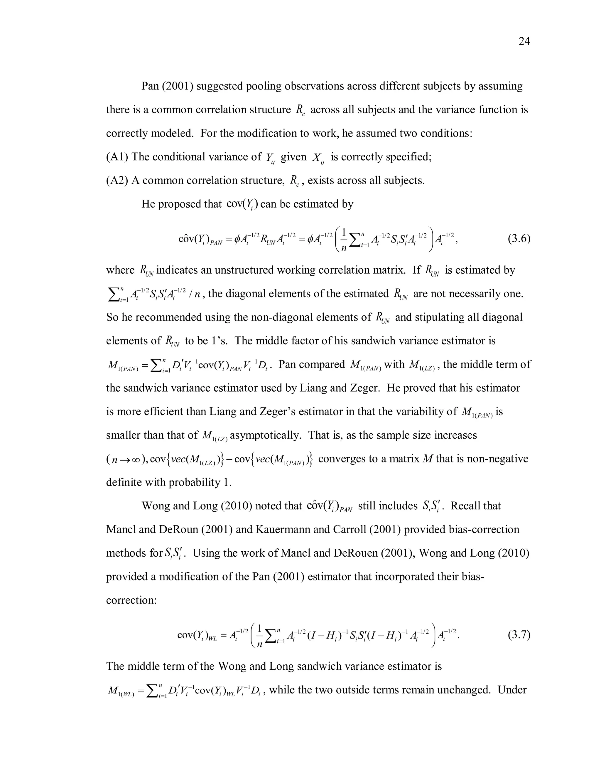
Likewise, the use of ˆjke on the working correlation matrix estimation in GEE
yields biased estimates of the variance. When ˆjke is used to estimate R(α) and cov( )iY ,
the sandwich variance estimator is negatively biased. Thus, several bias-corrected
sandwich variance estimators have been proposed (Mancl and DeRouen, 2001;
Kauermann and Carroll, 2001; Pan, 2001; Wong and Long, 2010) to improve the
estimation ofcov( )iY . Their definitions and properties are described in Section 3.2.
On the other hand, the biasedness of ˆ has not received much attention.
Recently, Lu et al. (2007) proposed a bias-corrected estimator for  . They provided
bias-corrected covariance estimates that extend those of Mancl and DeRouen (2001) to
encompass the correlation parameters as well as the mean parameters. Their proposed
estimating equation for  is
1
1
( ( )) 0,
n
i i i ii
S W R  

   (2.15)
where 12 13 ( 1)( , ,..., )i i i i m mR    
 is a [0.5 ( 1)] 1m m  vector with elements
( )ijk ij ikg s j k   . The row vector ijg corresponds to the jth row of the symmetric

45. 18
matrix 1/2 1/2 1
( )i i i iG I V H V  
  and iks is the kth column vector of ˆ ˆ( )( )i i i i iS Y Y     .
The matrix  
1
1
1
n
i i i i i i ii
H D D V D D V



   is called the cluster leverage by Preisser and
Qaqish (1996). A weighting matrix 12 13 ( 1)diag( , ,..., )i i i i m mW w w w  is a diagonal matrix
with elements ijkw , which is the variance of ˆ ˆij ike e (Prentice, 1988):
2
1/2
ˆ ˆ(1 2 )(1 2 )
1 .
( )
ij ik ijk
ijk ijk
ij ik
w
v v
  

 
   (2.16)
The estimating equations approach given by equation (2.15) to estimate the  parameters
in the vector ( )i  for the binary data case is implemented in the SAS/IML software
(http://www.bios.unc.edu/~jpreisse).
The performance of the bias-corrected α estimation by Lu et al. (2007) has not
been sufficiently investigated. Since iG includes R(α), derivation of the quantity of bias
correction needed for α estimation is not straightforward. Moreover, their method is
based on Mancl and DeRouen’s bias correction method, which has a tendency to
overcorrect the bias of the sandwich variance estimator. Therefore, it is not clear how
well their bias-corrected ˆ performs.
This dissertation is more focused on the selection of the working correlation
matrix structure rather than accuracy of the estimation of individual components working
correlation matrix. Therefore, Liang and Zeger’s approach for estimating  based on
Pearson residuals will be used throughout this dissertation. However, future work
includes an assessment of whether implementing a bias-corrected estimator of the 
vector has any impact on the ability to select an appropriate working correlation structure.

46. 19
CHAPTER 3
THE IMPORTANCE OF THE WORKING CORRELATION
STRUCTURE SELECTION
In the GEE method, if the working covariance matrix is correctly specified, along
with correct model specification, the  estimate becomes optimal within this asymptotic
framework and GV , the limiting covariance matrix of the regression  parameters, is
reduced to optV :
 
1
1
1
lim .
n
opt i i iin
V n DV D



  (3.1)
For any working covariance matrix, G optV V is a non-negative definite matrix (Wang and
Lin, 2005). Therefore, a misspecified working covariance matrix results in a loss of
efficiency.
Nevertheless, the modeling of ( )R  has not received much attention. In small
samples, a parsimonious structure with no parameters (independence) or one parameter
has been preferred by many researchers, since extra nuisance parameters can cause less
accurate estimates with high variability. Recently, several bias-corrected sandwich
variance estimators have been developed in order to improve the statistical efficiency
regardless of the choice of the working correlation structure in small samples.
In this section, the effect of misspecification of the working correlation structure
on the statistical efficiency is presented. First, the literature review on the asymptotic
relative efficiency of the variance estimator under misspecified working correlation
structure is presented. Later, several bias-corrected sandwich variance estimators are
introduced. Then, the sensitivity of the bias-corrected sandwich variance estimator to the
misspecified working correlation structure is evaluated using a simulation study.

47. 20
3.1 Asymptotic Relative Efficiency of the Variance
Estimator under the Misspecified Working Correlation
Structure
Asymptotic relative efficiency (ARE) for a regression parameter estimator is
defined as the ratio of the appropriate diagonal element in the “optimal” estimation
variance and the corresponding “working” estimation variance. That is, the numerator of
ARE is the diagonal element in optV and the denominator is the diagonal element in GV
under a misspecified working correlation structure corresponding to a single  parameter
(Wang and Lin, 2005). Some simulation studies use GV under the independence
assumption to compute the ARE.
Since the analytical expression for asymptotic relative efficiency is not available
in general, many simulation studies reported in the literature were carried out to evaluate
the amount of the efficiency loss observed. Among those simulation studies, however,
there have been some controversies regarding the efficiency loss resulting from the
misspecified working covariance matrix. For instance, Zhao and Prentice (1990) and
Liang et al. (1990) showed in their simulation studies that the variance estimators under
INR (independence working correlation) were similar to those under the true correlation
structure, although there was a little efficiency loss. On the other hand, Liang and Zeger
(1986), Zhao et al. (1992), Fitzmaurice (1995) and Wang and Carey (2003) showed that
the loss of efficiency due to the misspecification of the working correlation matrix
depended on both the strength of the correlation between the responses and the covariate
design matrix. If the true correlation was small to moderate, the sandwich variance
estimators were similar, regardless of the choice of working correlation structure. If the
true correlation was high, the substantial improvement in statistical efficiency could be
obtained by correctly specifying the working correlation structure. If the covariate design
includes at least one within-cluster covariate, the independence assumption can lead to a
substantial loss of efficiency. Therefore, Fitzmaurice et al. (2004) and other authors

48. 21
recommended some attempt should be made to model within-subject association
correctly, even though those parameters are regarded as a nuisance parameters and the
true underlying correlation structure is unknown.
Nevertheless, there are some practical concerns regarding the working correlation
selection in small samples. McDonald (1993) described a concern that if the sample sizes
were small, the extra nuisance parameters could cause convergence difficulties and
inflate the variances, even if the specification of the nuisance parameters was correct.
For these reasons, parsimonious working correlation structures with one or zero
parameters have been favored by many researchers.
3.2 Bias-Corrected Sandwich Variance Estimators
Recently, new attempts to estimate the asymptotic variance of  more precisely
by removing inherent bias has been made to improve the efficiency, regardless of the
choice of the working correlation structure in small samples. In this section, several bias-
corrected sandwich variance estimators are introduced.
It has been widely-known that the sandwich variance estimator proposed by Liang
and Zeger (1986) is biased downward and generally has a larger variability than the
model-based variance estimator (Paik, 1988; Sherman and le Cessie, 1997; Kauermann
and Carroll, 2001; Mancl and DeRouen, 2001; Lu et al., 2007; Wong and Long, 2010).
Use of the negatively-biased variance estimator can result in the hypothesis tests of the
regression coefficients that are too liberal and confidence intervals on the s that are too
narrow, especially in smaller samples. So, various alternative estimators to the GEE
sandwich estimator have been proposed (Paik, 1988; Lipsitz et al., 1990; Qu et al., 1994;
Sherman and le Cessie, 1997; Kauermann and Carroll, 2001; Mancl and DeRouen, 2001;
Pan, 2001; Wong and Long, 2010). Among them, four recent approaches will be
described.

49. 22
Kauermann and Carroll (2001) showed that the sandwich variance estimator used
by Liang and Zeger (1986) under the correctly specified working covariance is negatively
biased with order 1/n and proposed a bias-corrected sandwich variance estimator
assuming a correctly specified variance structure. Their estimators for cov( )iY and the
bias-corrected sandwich variance estimator (KC) are presented in equations (3.2) and
(3.3).
   
1/2 1/2
ˆ ˆˆ ˆ ˆcov( ) ( )( ) ,i KC i i i ii i
Y Y YI H I H 
 
    (3.2)
where  
1
11
1
n
i i i ii i ii
H D D VD V D



  is called the cluster leverage (Preisser and Qaqish,
1996).
   
1 1
1 1 1 1
1 1 1
ˆ ˆ ˆ ˆ ˆ ˆ ˆ ˆ ˆ ˆ .ˆcov( )
n n n
i i i i i i KC i i i i ii i i
KC D V D D V Y V D D V D
 
   
  
        (3.3)
Mancl and DeRouen (2001) proposed another bias-corrected sandwich variance
estimator. Unlike Kauermann and Carroll (2001), they did not assume a correctly
specified working covariance and ignored one term from its first order expansion
resulting in overcorrection. Thus, the proposed estimator of Mancl and DeRouen tends to
overcorrect the bias. Mancl and DeRouen’s bias-corrected ˆcov( )iY and their sandwich
variance estimator (MD) are presented in the equations (3.4) and (3.5).
   
1 1
ˆ ˆˆ ˆ ˆcov( ) ( )( ) .i MD i i i ii i
Y Y YI H I H 
 
    (3.4)
   
1 1
1 1 1 1
1 1 1
ˆ ˆ ˆ ˆ ˆ ˆ ˆ ˆ ˆ ˆ .ˆcov( )
n n n
i i i i i i MD i i i i ii i i
MD D V D D V Y V D D V D
 
   
  
        (3.5)
Note the difference between these two estimators. Kauermann and Carroll included the
term  
1/2
ˆ
iI H

 in their expression for ˆcov( )iY , whereas Mancl and DeRouen used
 
1
ˆ
iI H

 instead.
Lu et al. (2007) compared the small sample performance of these two bias-
corrected sandwich variance estimators. The marginal mean model and the within-cluster
correlations were correctly specified in their simulation study. They considered the

50. 23
correlated binary data setting with the several balanced cluster sizes (m=4, 6, 10, 40, 80)
and sample sizes (n=10, 14, 20, 40, 80). The marginal mean model they used was
0 1 1 2 2 3 1 2logit( ) ,ij ij ij ij ijX X X X       
where 1 =1ijX for an intervention community and 0 for a control community; 2 =1ijX for
posttest (year1), and 0 for baseline (pretest) and 0 1 2 3( , , , ) (0.25,0, 0.1, 0.3) .        
The true correlation structure was defined by 0 10.10 0.05ijj ijj jj jjz z z       where
(1, 0)ijjz   if 2 2ij ijX X  and (0,1)ijjz   if 2 2ij ijX X  . To evaluate the performance of the
variance estimators, the marginal mean model was fixed. An evaluation of 1
ˆˆvar( ),
2 3
ˆ ˆˆ ˆvar( ) and var( )  comparing the two bias-correction approaches to each other and to the
original Liang and Zeger sandwich estimator was presented. When the sample size was
less than 40, the Mancl and DeRouen (MD) estimator consistently overestimated the
three variances and was more variable than the Kauermann and Carroll (KC) and the
Liang and Zeger (LZ) sandwich estimators. With respect to the bias reduction in the
estimation of ˆcov( ) , the KC estimator performed better than the MD estimator.
However, the MD estimator had better coverage probabilities than the KC estimator.
This is because the overcorrection of the negative bias is offset by the greater chance of
undercoverage resulting from the high variability of the sandwich estimator.
Pan (2001) suggested a different approach for estimating the cov( )iY term in the
sandwich variance estimator. Recall that the original Liang and Zeger (1986)
proposalwas to estimate cov( )iY by i iS S where ˆ ˆ( )( )i i i i iS Y Y     . Mancl and
DeRouen (2001) and Kauermann and Carroll (2001) estimate cov( )iY by
1 1
( ) ( )i i i iI H S S I H 
  and 1/2 1/2
( ) ( )i i i iI H S S I H 
  , respectively. One common
characteristic of these estimators is that the estimate of cov( )iY is based only on the
estimated deviations ˆ ˆ( )( )i i i i iS Y Y     from subject i, rather than pooling across
subjects, as proposed by Pan (2001) and others

51. 24
Pan (2001) suggested pooling observations across different subjects by assuming
there is a common correlation structure cR across all subjects and the variance function is
correctly modeled. For the modification to work, he assumed two conditions:
(A1) The conditional variance of ijY given ijX is correctly specified;
(A2) A common correlation structure, cR , exists across all subjects.
He proposed that cov( )iY can be estimated by
1/2 1/2 1/2 1/21/2 1/2
1
1
ˆcov( ) ,
n
i PAN i UN i i ii i i ii
Y A R A A AA S S A
n
     

    
 
 (3.6)
where UNR indicates an unstructured working correlation matrix. If UNR is estimated by
1/2 1/2
1
/
n
i i i ii
A S S A n 

 , the diagonal elements of the estimated UNR are not necessarily one.
So he recommended using the non-diagonal elements of UNR and stipulating all diagonal
elements of UNR to be 1’s. The middle factor of his sandwich variance estimator is
1 1
1( ) 1
cov( )
n
PAN i i i PAN i ii
M D V Y V D 

  . Pan compared 1( )PANM with 1( )LZM , the middle term of
the sandwich variance estimator used by Liang and Zeger. He proved that his estimator
is more efficient than Liang and Zeger’s estimator in that the variability of 1( )PANM is
smaller than that of 1( )LZM asymptotically. That is, as the sample size increases
( n ),    1( ) 1( )cov ( ) cov ( )LZ PANvec M vec M converges to a matrix M that is non-negative
definite with probability 1.
Wong and Long (2010) noted that ˆcov( )i PANY still includes i iS S. Recall that
Mancl and DeRoun (2001) and Kauermann and Carroll (2001) provided bias-correction
methods for i iS S. Using the work of Mancl and DeRouen (2001), Wong and Long (2010)
provided a modification of the Pan (2001) estimator that incorporated their bias-
correction:
1/2 1/21/2 1 1 1/2
1
1
cov( ) .( ) ( )
n
i WL i ii i i i i ii
Y A AA I H S S I H A
n
    

    
 
 (3.7)
The middle term of the Wong and Long sandwich variance estimator is
1 1
1( ) 1
cov( )
n
WL i i i WL i ii
M D V Y V D 

  , while the two outside terms remain unchanged. Under

52. 25
the usual regulatory conditions for GEE and assumptions (A1) and (A2), they showed
that 1( ) 1( )cov( ( )) cov( ( ))LZ WLvec M vec M and 1( ) 1( )cov( ( )) cov( ( ))MD WLvec M vec M are both
non-negative definite matrices with probability 1, while
1( ) 1( )cov( ( )) cov( ( )) 0PAN WLvec M vec M  with probability 1 as .n   This implies that
Wong and Long’s estimator and Pan’s estimator are asymptotically equivalent in terms of
the variability of their estimators. However, Wong and Long’s estimator is
asymptotically less variable than those proposed by Liang and Zeger and Mancl and
DeRouen.
3.3 Simulation Study I: The Performance of the Bias-
Corrected Sandwich Variance Estimators under
Misspecified Working Correlation Structures
The performance of the bias-corrected sandwich variance estimators described in
Section 3.2 has been evaluated in the literature under somewhat limited conditions.
When the true correlations among responses were low, the bias-corrected sandwich
variance estimators were not sensitive to the misspecification of the working correlation
structure. However, in most simulations, only very parsimonious working correlation
structures with zero or one parameter were considered. Moreover, the impact of the
strength of the true correlations among responses on the performances of the bias-
corrected sandwich variance estimators was not assessed.
Simulation Study I is aimed at evaluating the performance of the bias-corrected
sandwich variance estimators in various settings. Five working correlation structures
(independence, exchangeable, AR-1, Toeplitz and unstructured), different sample sizes,
cluster sizes, and true correlation structures are considered. As the correct specification
of the mean model is not the focus of this dissertation, all simulation studies will use the
same, simple, and correctly-specified mean model.

53. 26
3.3.1 Simulation Setting
This simulation study addresses the performance of the six variance estimators
described more fully above when the sample size is relatively small:
1. The model-based variance estimator of Liang and Zeger (MB)
2. The sandwich variance estimator by Liang and Zeger (LZ)
3. The bias-corrected sandwich variance estimator of Kauermann and Carroll (KC)
4. The bias-corrected sandwich variance estimator by Mancl and DeRouen (MD)
5. The bias-corrected sandwich variance estimator by Pan (PAN)
6. The bias-corrected sandwich estimator of Wang and Long (WL).
The simulation design has a factorial design, with the factor levels as described in
Table 3.1. For each cell of the study, 1000 random samples are generated, and all
estimators are computed using the same data from each sample drawn. The marginal
mean model is correctly modeled.
Since AR-1 and EX correlation matrices only depend on one α parameter, they
are simple to define. On the other hand, TOEP and UN correlation structures require
 1m  and ( 1)/ 2m m parameters, respectively. Note that the AR-1 and exchangeable
structures are nested within the Toeplitz structure, and all patterned matrices are nested
within the unstructured matrix form. The form of the underlying, true Toeplitz and
unstructured correlation structures were chosen to be distinct from other candidate forms,
and the structure for the m m matrix was chosen to be nested within that of the
( 1) ( 1)m m   matrix, m=4, 6, as shown in Table 3.2(a) and Table 3.2 (b).

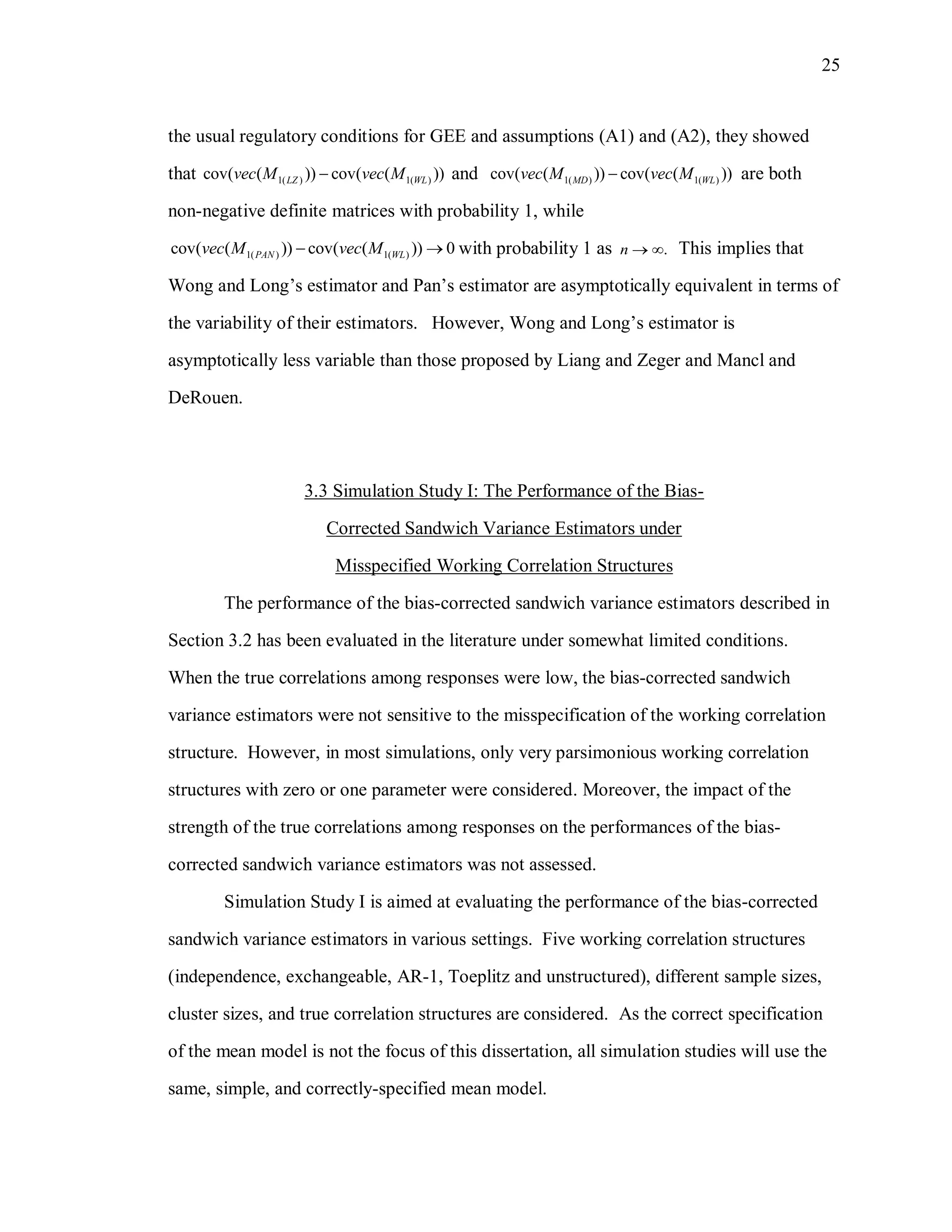
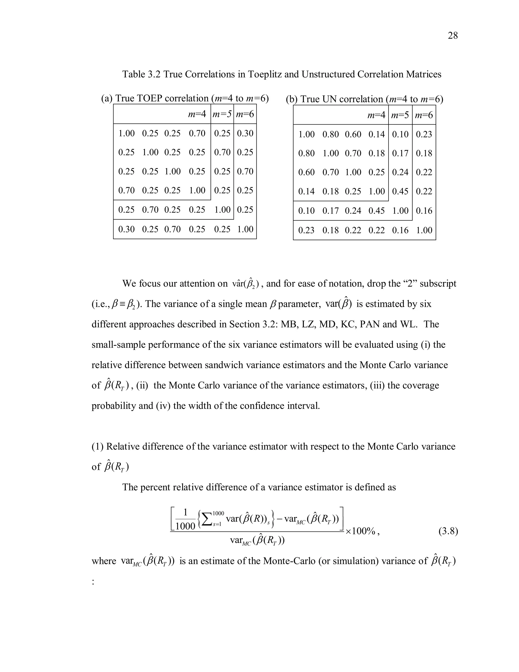
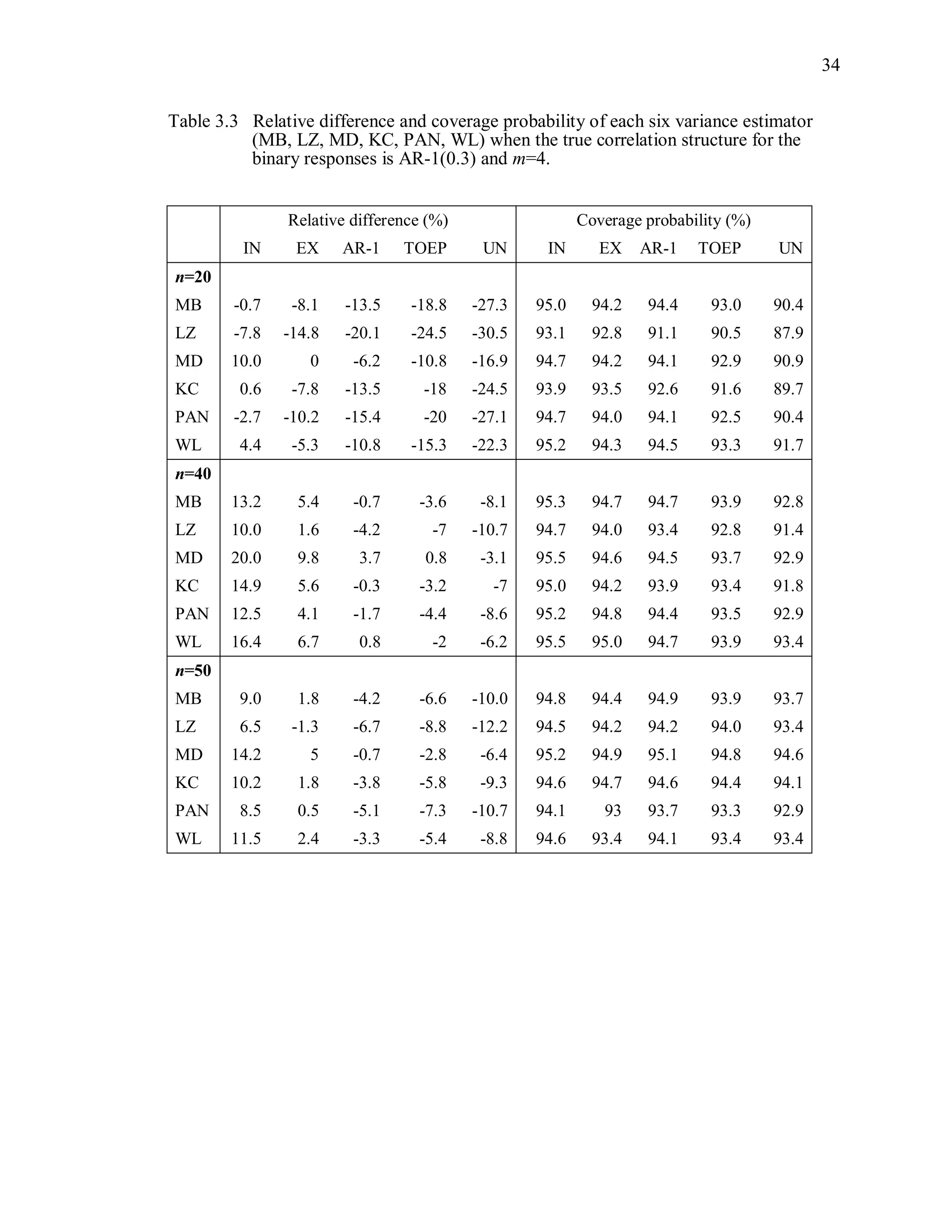
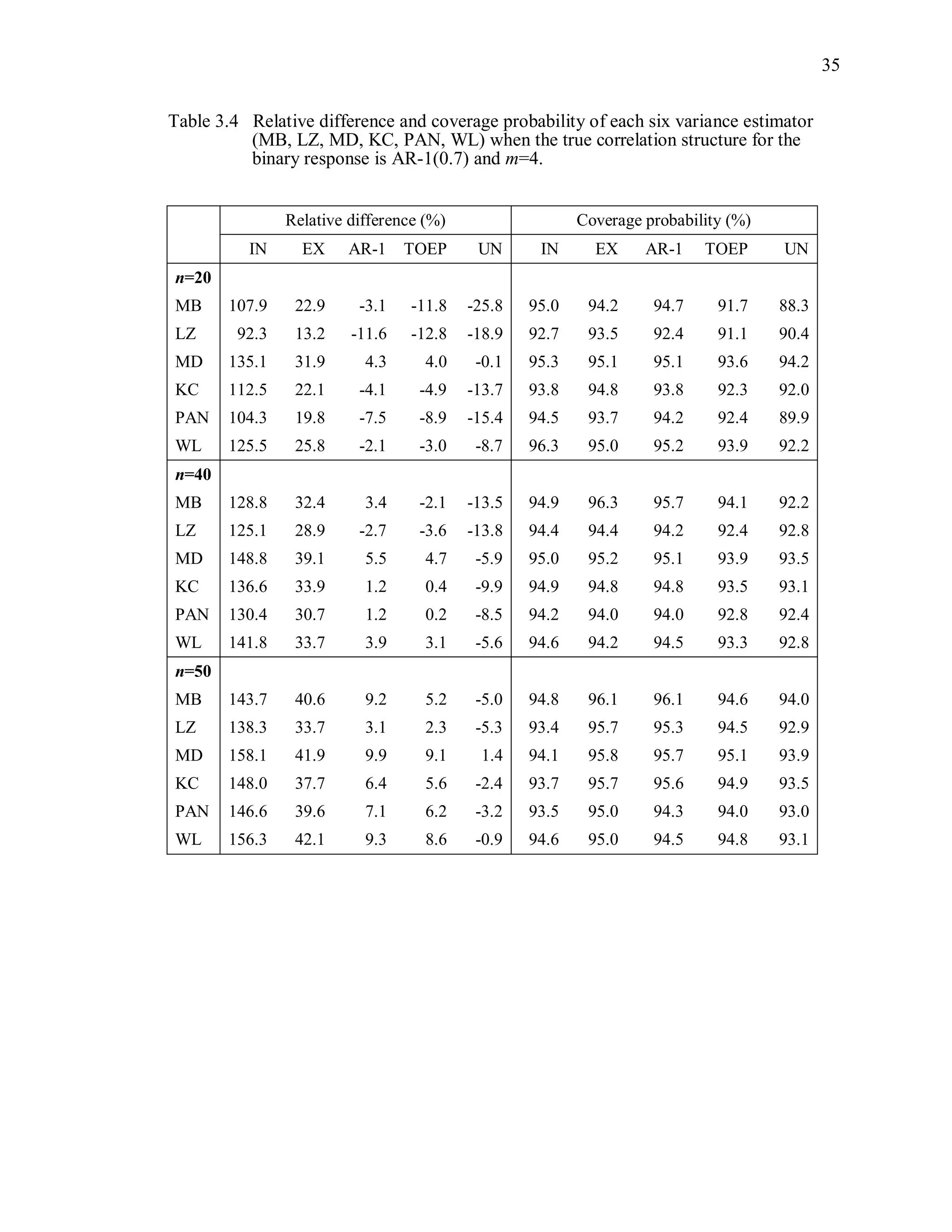
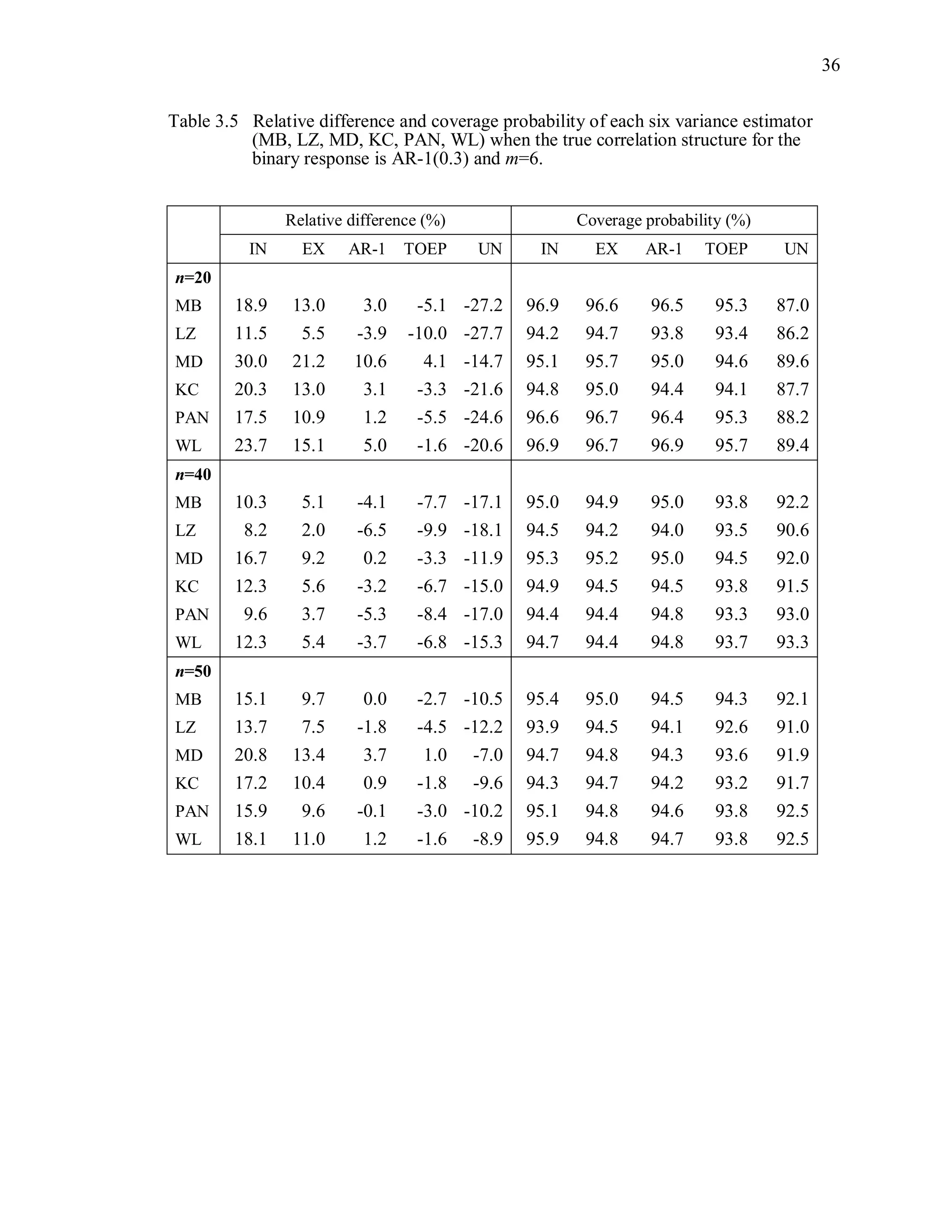
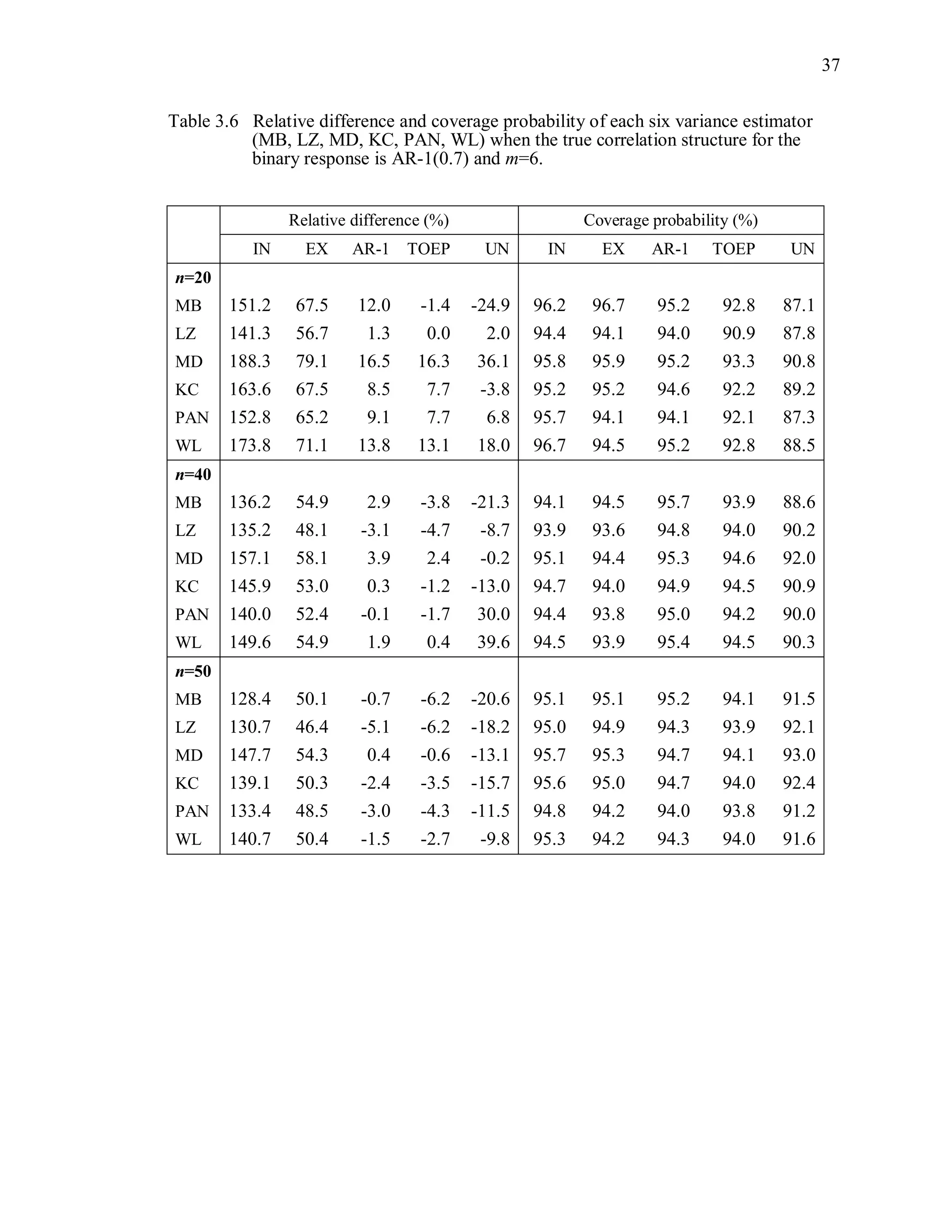
54. 27
Table 3.1 Simulation Study I Design Parameters
Factor Levels
Distribution (D) Multivariate Bernoulli responses:
1 1 2 2logit( ) ,it t tx x    where 1tx and 2tx are
independently generated from U[0.5, 1],
1 2 0.3.  
Response vector dimension (m) 4, 6m 
True Correlation Structure
( )C 
Exchangeable: EX(α), α=0.3, 0.7
Autoregressive of order 1: : AR-1(α), α=0.3, 0.7
Toeplitz: TOEP(m), : α values in Table 3.2(a)
Unstructured: UN(m), : α values in Table 3.2(b)
Working Correlation structure
( )R 
Independence (IN), Exchangeable (EX),
Autoregressive (AR-1), Toeplitz (TOEP), and
unstructured (UN)
Variance Estimator for 2
ˆ MB, LZ, KC, MD, PAN, WL
Sample Sizes (n) n = 20, 40, 50

55. 28
Table 3.2 True Correlations in Toeplitz and Unstructured Correlation Matrices
(a) True TOEP correlation (m=4 to m=6)
m=4 m=5 m=6
1.00 0.25 0.25 0.70 0.25 0.30
0.25 1.00 0.25 0.25 0.70 0.25
0.25 0.25 1.00 0.25 0.25 0.70
0.70 0.25 0.25 1.00 0.25 0.25
0.25 0.70 0.25 0.25 1.00 0.25
0.30 0.25 0.70 0.25 0.25 1.00
(b) True UN correlation (m=4 to m=6)
m=4 m=5 m=6
1.00 0.80 0.60 0.14 0.10 0.23
0.80 1.00 0.70 0.18 0.17 0.18
0.60 0.70 1.00 0.25 0.24 0.22
0.14 0.18 0.25 1.00 0.45 0.22
0.10 0.17 0.24 0.45 1.00 0.16
0.23 0.18 0.22 0.22 0.16 1.00
We focus our attention on 2
ˆˆvar( ) , and for ease of notation, drop the “2” subscript
(i.e., 2  ). The variance of a single mean  parameter, ˆvar( ) is estimated by six
different approaches described in Section 3.2: MB, LZ, MD, KC, PAN and WL. The
small-sample performance of the six variance estimators will be evaluated using (i) the
relative difference between sandwich variance estimators and the Monte Carlo variance
of ˆ( )TR , (ii) the Monte Carlo variance of the variance estimators, (iii) the coverage
probability and (iv) the width of the confidence interval.
(1) Relative difference of the variance estimator with respect to the Monte Carlo variance
of ˆ( )TR
The percent relative difference of a variance estimator is defined as
 1000
1
1 ˆ ˆvar( ( )) var ( ( ))
1000 100% ,
ˆvar ( ( ))
s MC Ts
MC T
R R
R
 


 
   

(3.8)
where ˆvar ( ( ))MC TR is an estimate of the Monte-Carlo (or simulation) variance of ˆ( )TR
:

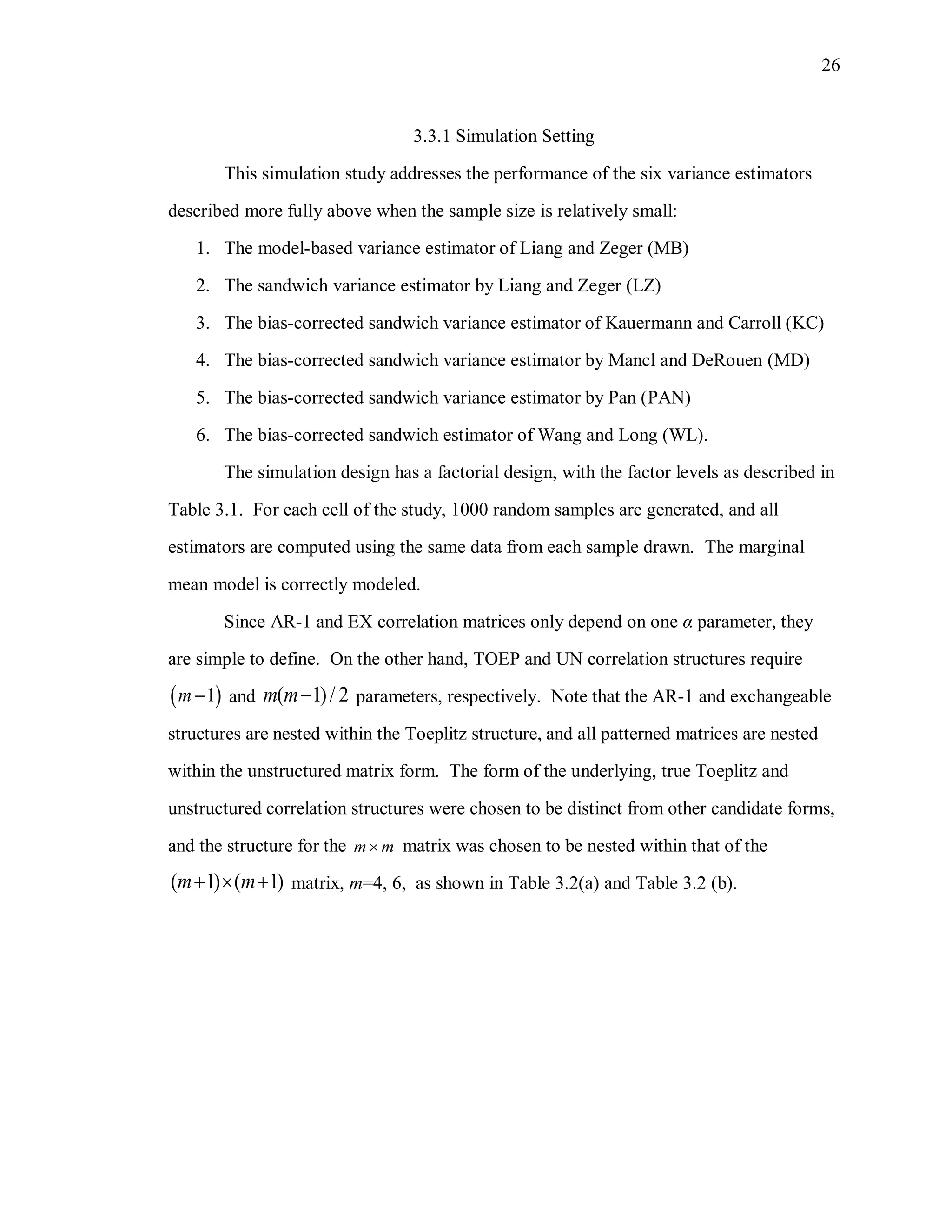
56. 29
2
1000 1000
1 1
1 1ˆ ˆ ˆvar ( ( )) .( ) ( )
999 1000
MC T T s T ss s
R R R   
 
  
 
  (3.9)
(2) Monte Carlo variance of the variance estimator
The Monte Carlo variance of the variance estimator is calculated by
2
1000 1000
1 1
1 1ˆ ˆ ˆvar [var( ( ))] var( ( )) var( ( )) .
999 1000
MC s ss s
R R R   
 
  
 
  (3.10)
where ˆvar( ( ))sR is the estimated variance of ˆ under the working correlation structure
R from the sth
simulation.
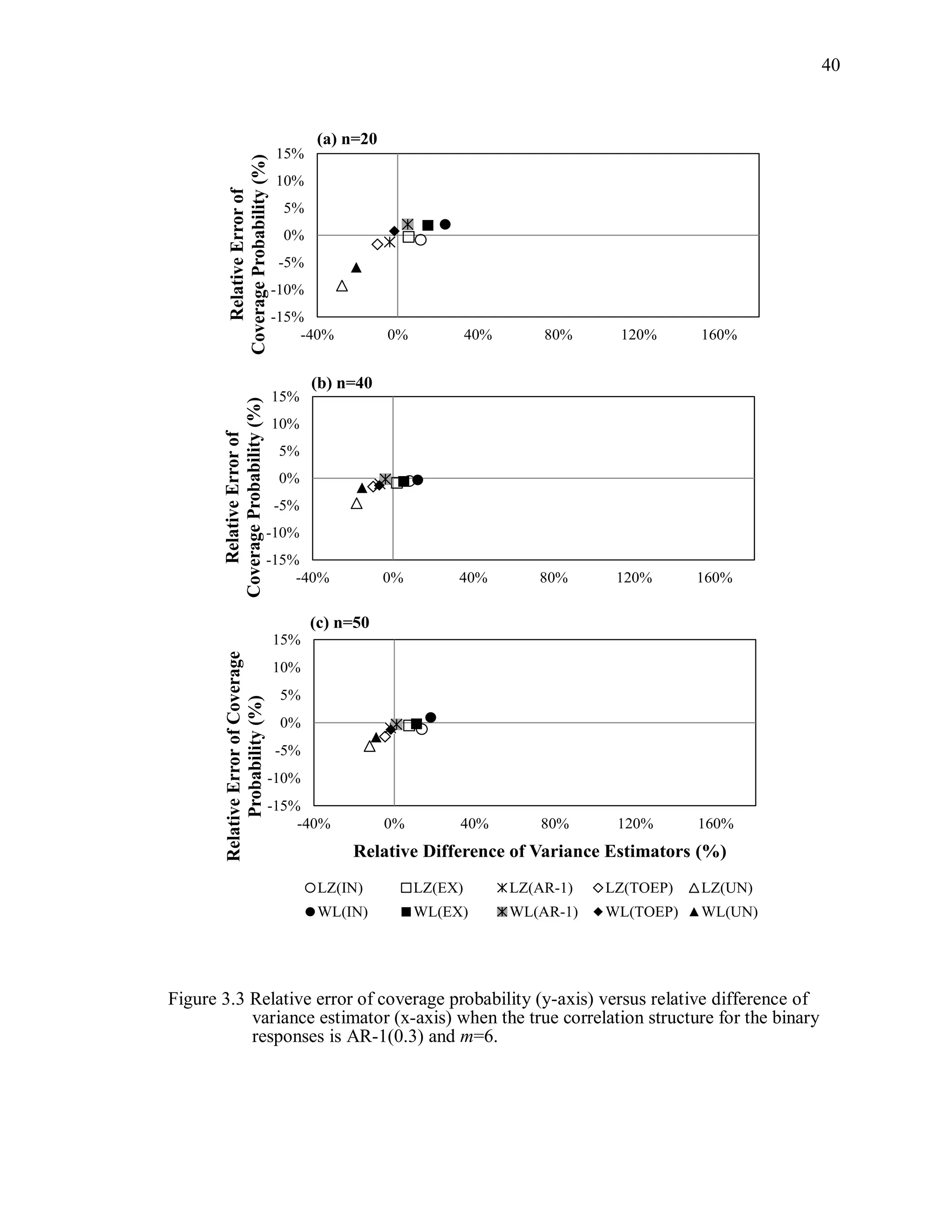
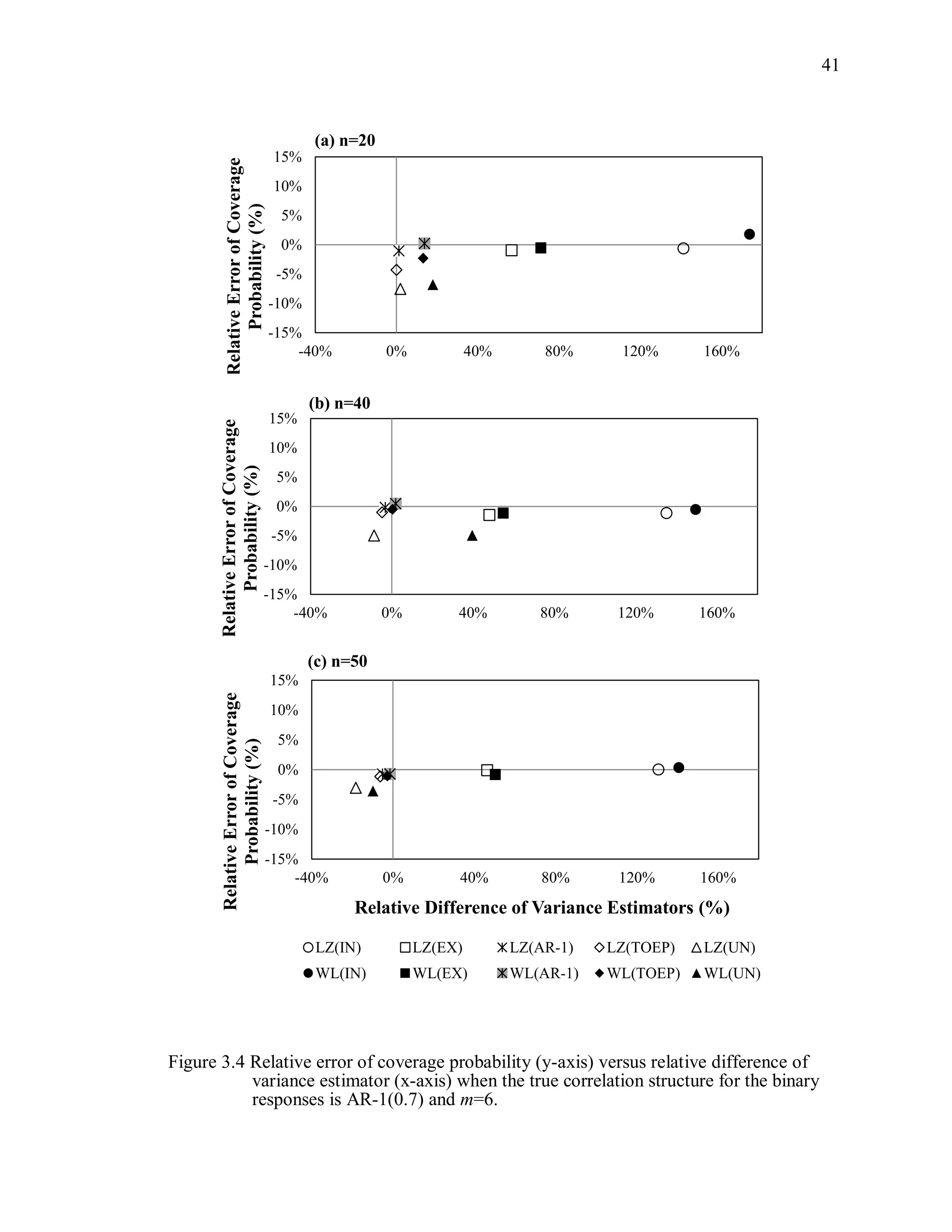
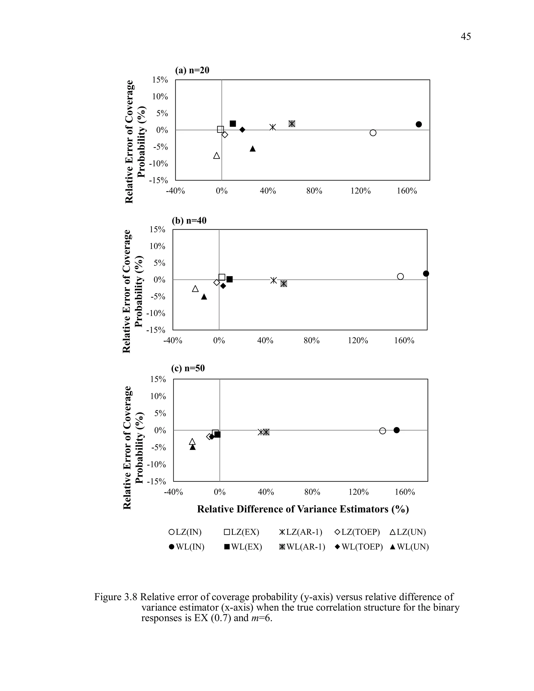
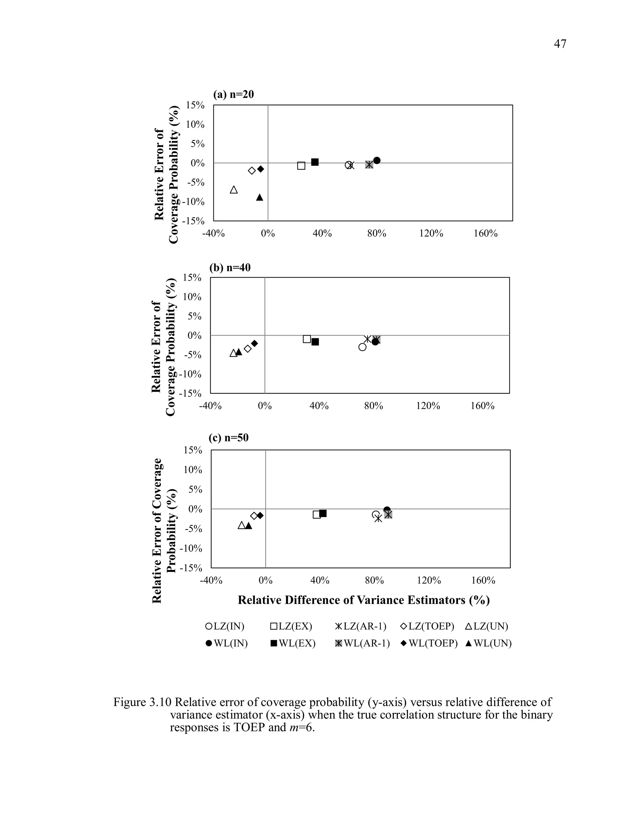
(3) Coverage probability and relative error of the coverage probability
Coverage probability is defined as the probability that a 95% Wald-type
confidence intervals for , using the working correlation structure R, from 1000
simulations will contain the true parameter:
ˆ ˆ ˆ ˆˆP[ ( ) 1.96 var( ( )) 1.96 var( ( ))] .CP R R R         (3.11)
The estimated coverage probability is the proportion of 95% confidence intervals
computed as ˆ ˆ( ) 1.96 cov( ( ))R R  that contain the true parameter value β. The
relative error of the coverage probability is defined as
( 0.95)/ 0.95 100%.CP  (3.12)
(4) Width of the confidence interval
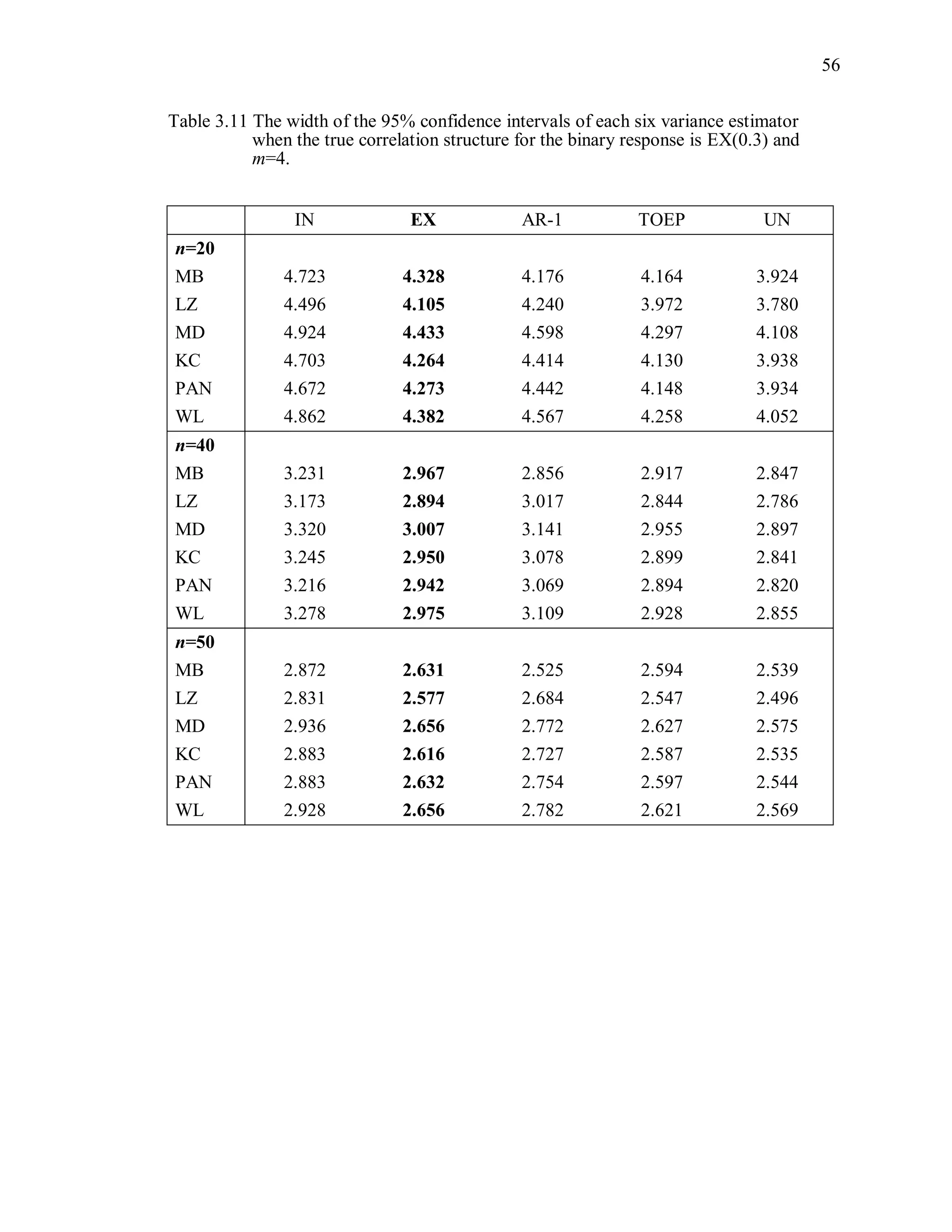
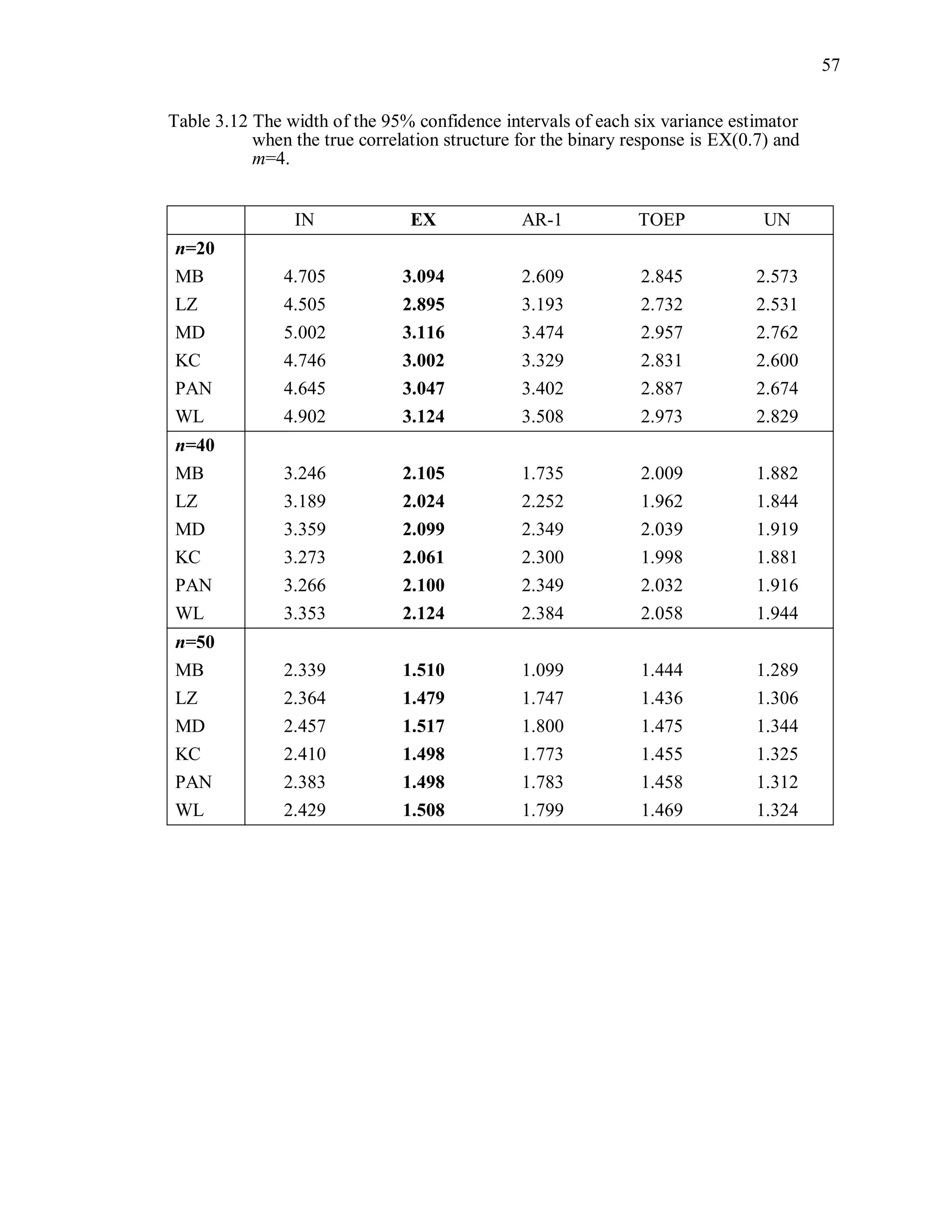
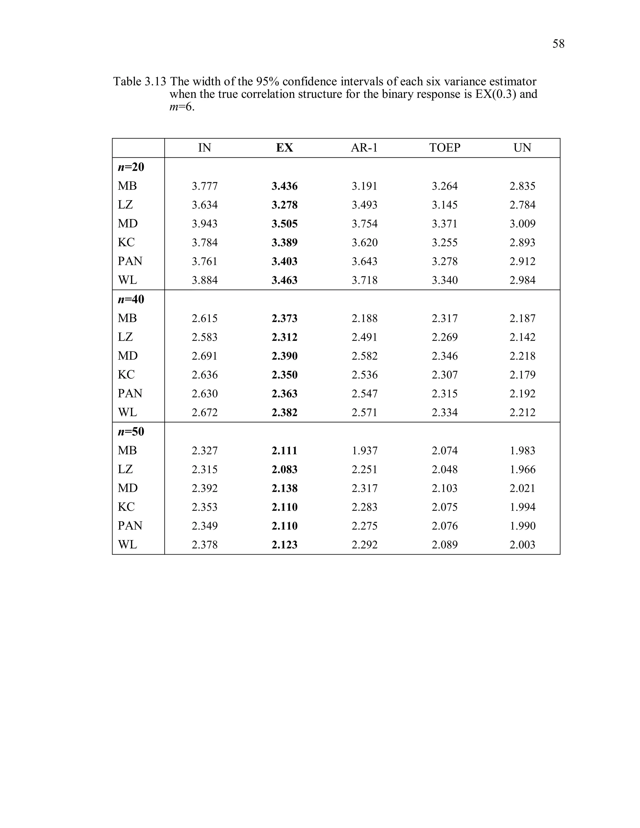
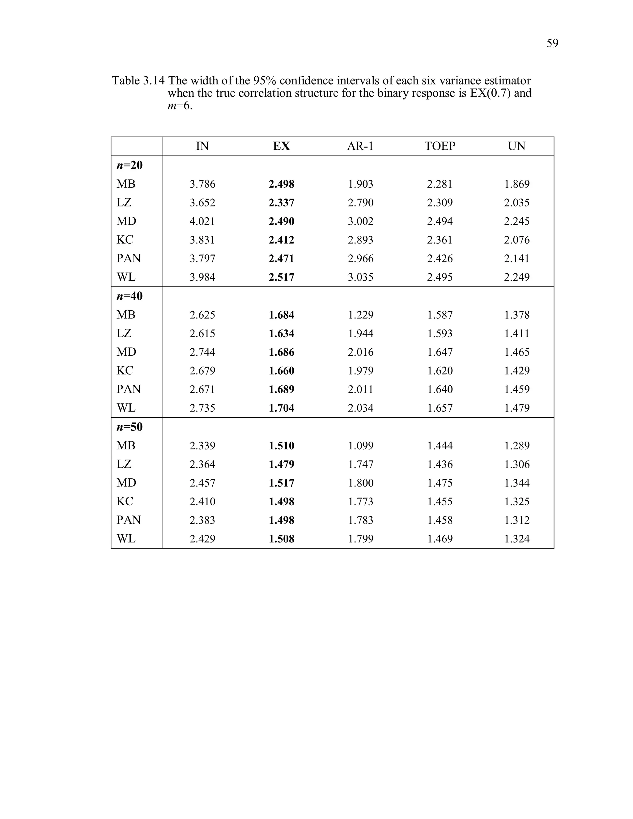
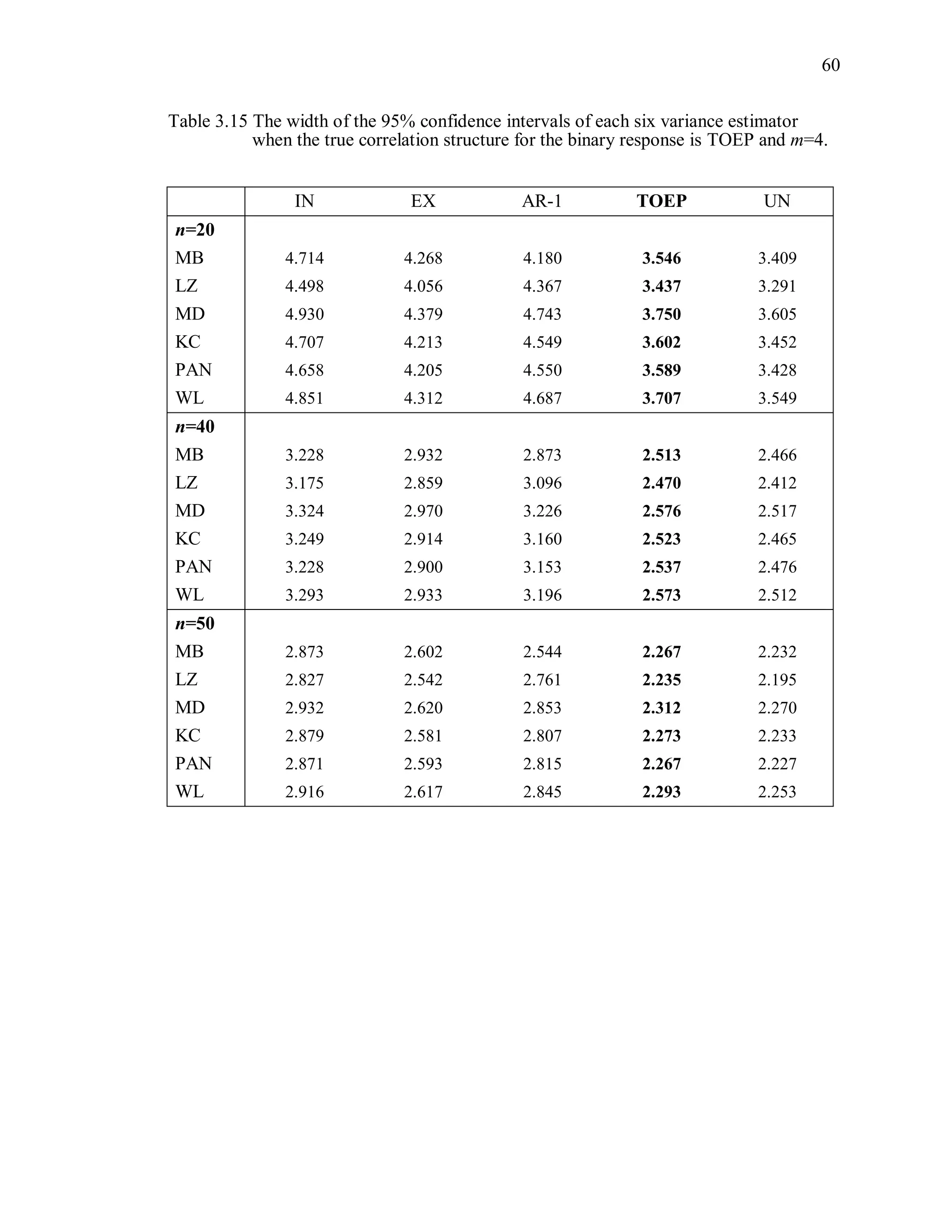
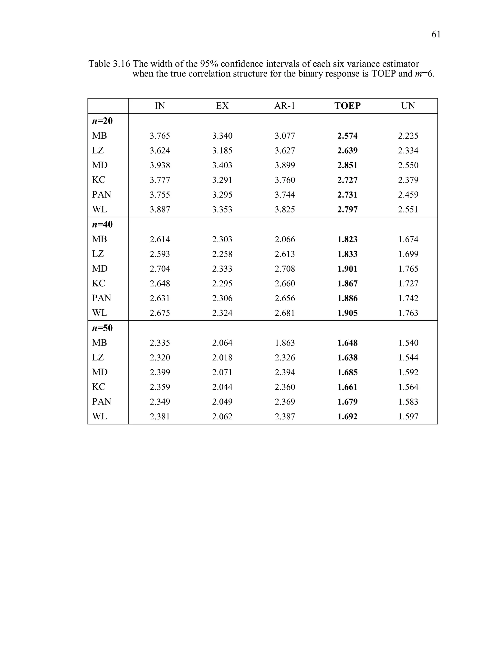
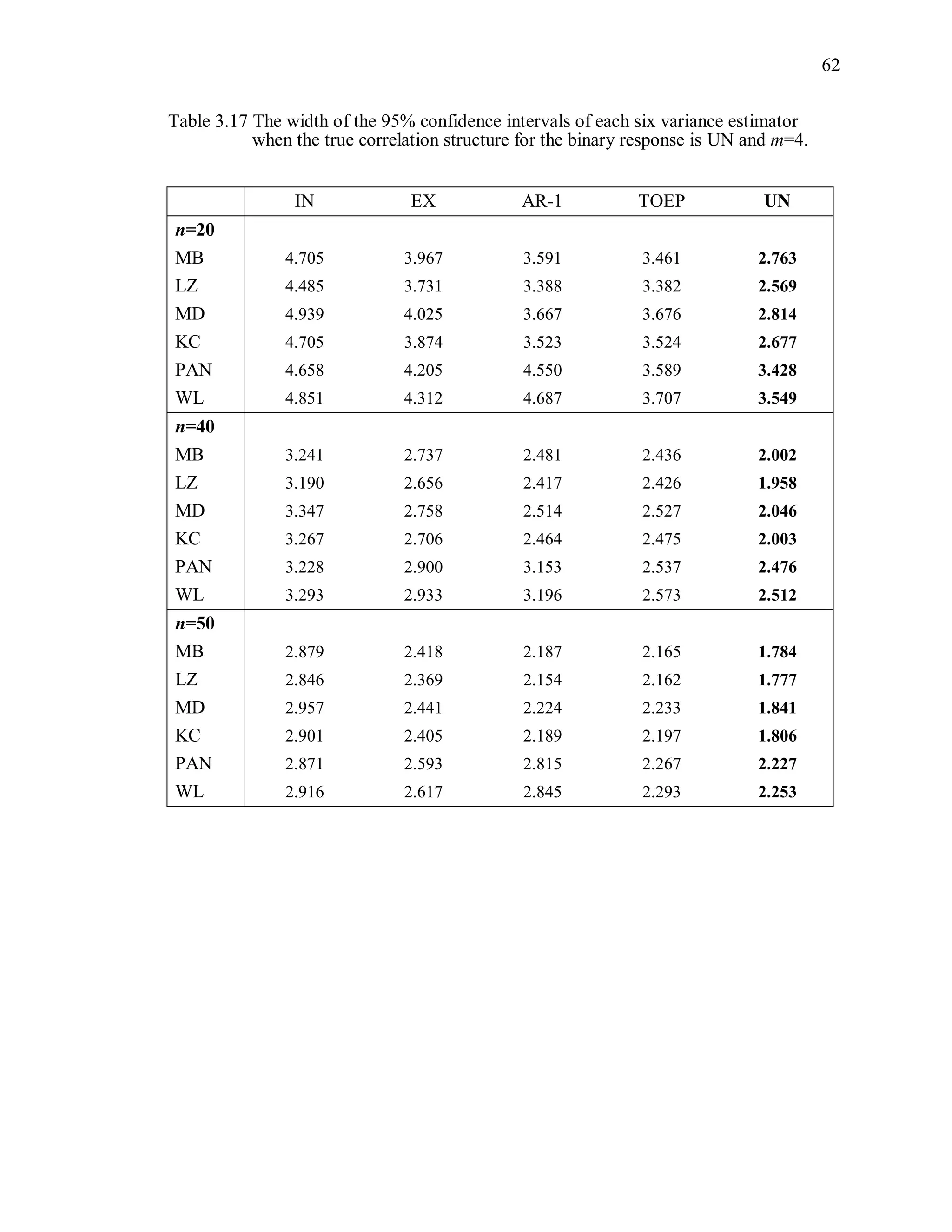
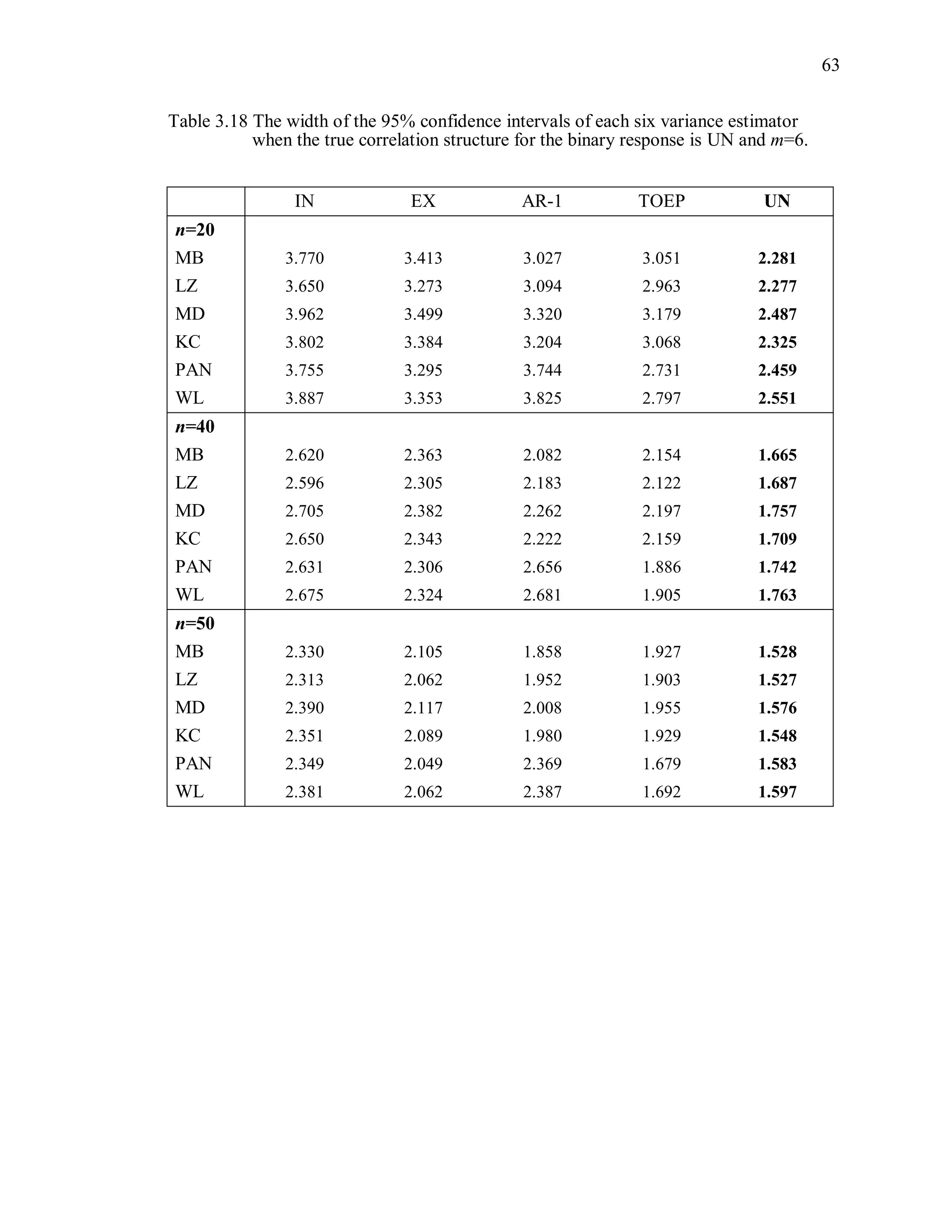
The width of the 95% Wald confidence interval is defined as
ˆ2 1.96 var( ( )) .R  (3.13)
For each variance estimator, the average of the widths of the confidence intervals from
1000 independent simulations is computed.

57. 30
3.3.2 Simulation Results
Table 3.3 through Table 3.6 provide the relative difference and coverage
probability of all six variance estimators when the data are binomial and the true
correlation matrix is AR-1 (  0.3, 0.7 and m = 4, 6). Corresponding simulation results
for cases where the true correlation matrix is independence (IN), exchangeable (EX),
Toeplitz, or Unstructured are shown in Appendix A (Tables A.1-A.8), but are discussed
below. Figure 3.1 through Figure 3.12 present the scatter plots of the relative difference
against the relative error of the coverage probability of the two sandwich variance
estimators (LZ and WL) under the five working correlation structures (IN, AR-1, EX,
Toeplitz, and Unstructured). Other bias-corrected sandwich variance estimators are
omitted from the figures because they show patterns that are very similar to the WL
estimator, and would be difficult to distinguish on the plots. The first four figures (Figure
3.1 – Figure 3.4) are from simulations in which AR-1 is the correct model. Figure 3.5
through Figure 3.8 correspond to cases where exchangeable is the correct underlying
model. Since the  parameters for the Toeplitz and unstructured correlation matrices
when m =4 are embedded in that for m =6, only two figures are needed for cases where
the underlying true correlation is Toeplitz (Figure 3.9, Figure 3.10) or unstructured
(Figure 3.11, Figure 3.12). In each scatter plot, the closer the point is to the origin, the
closer the variance estimator approximates the asymptotic variance of  , since both the
relative difference and the relative error of the coverage probability are close to zero.
3.3.2.1 Relative Difference of the Variance Estimator
Overall, the direction and the magnitude of the relative difference of the variance
estimator depend on the true underlying correlation structure C(), the sample size (n),
the cluster size (m), and the choice of the working correlation structure.
If the working correlation structure is correctly specified or over-parameterized,
the amount of the relative difference of the six variance estimators decreases as n

58. 31
increases. However, under the misspecified working correlation structure, the relative
difference of the variance estimators does not necessarily decrease as n increases. For
instance, we see that the working independence matrix leads to a highly inflated ˆvar( ) ,
especially when the true α parameter is a high positive value (Table 3.4, Table 3.6, Figure
3.2, Figure 3.4, Figure 3.6, Figure 3.8).
Generally speaking, the three bias-corrected sandwich variance estimators (KC,
PAN, and WL) tend to have smaller relative difference as compared to the sandwich
variance estimator by Liang and Zeger (LZ). The MD estimator tends to overcorrect the
bias in comparison to other variance estimators in small samples, which is consistent with
the simulation results of Lu et al. (2007), and has more variability in its bias estimates.
The model-based estimator of Liang and Zeger under model misspecification has similar
relative difference as their sandwich estimator (LZ) when the dimension of the
covariance matrix is m=4, but performs worse when the dimension of the matrix is larger
(m =6).
The simulation results clearly indicate that the bias-corrected sandwich variance
estimators are not robust to the misspecification of the working correlation structure. If
the true pairwise correlations between the responses are low and the number of multiple
measurements is small, the variance estimates under the different misspecified working
correlation structures are similar (Figure 3.1, Figure 3.5). However, if the true pairwise
correlations between the responses are high, the misspecified working correlation
structures cause inflated variance estimates. For example, if the true correlation structure
is AR-1, the exchangeable and the independence working correlation structure do not
approximate the true correlation matrix, even in large samples. This results in a positive
bias, so the corresponding sandwich variance estimators tend to have inflated values.
The observed relative difference of the variance estimators under independence
assumption went up to 180%.

59. 32
The unstructured working correlation matrix yields more negatively-biased
variance estimates as compared to other working correlation matrices. The use of the
bias-corrected variance estimators does not fully overcome this negative bias when the
structure has a relatively large number of parameters which can be used to match any
particular data set. In particular, when the true correlations between the responses are
weak and the responses of the same individual are measured on many occasions, the
variance estimates under UNR tend to underestimate ˆvar( ) more severely than other
working correlation structures (Table 3.5).
Lastly, the relative difference of the model-based variance estimator using the
correctly specified working correlation structure is not always closest to zero, as one
might expect, due to variability in small samples. Even though the working correlation
structure is correctly specified, if the true correlation structure is complicated, the
parameter estimation can be inefficient in the smaller samples. Figure 3.11 and Figure
3.12 show that the variance estimates under UNR , which is the correctly specified
structure, are more negatively biased than the variance estimates under more
parsimonious structure such as TOEPR , for sample sizes of n=20 and n=40, but although
still negative, come closer to 0 for n=50 than the other under-parameterized structures.
3.3.2.2 Coverage Probability
Coverage probability appears to be less sensitive to the misspecification of the
working correlation structure than relative difference of the regression parameter variance
estimator. In this simulation study, the mean model is correctly specified, so the GEE
estimated regression parameter ( ˆ ) is close to the true value T . Unless the estimated
variance is too small (due primarily to the negative bias) or highly variable (due to small
sample sizes), the true parameter value is within the confidence interval. The
misspecified, but parsimonious working correlation structure sometimes results in the

60. 33
coverage probability close to the nominal value. For example, when C(α) is AR-1(0.3),
m=4, n=40 and the KC estimator is used (Table 3.3), the coverage probabilities under INR ,
EXR and 1ARR  are 95%, 94.2% and 93.4%, respectively. On the other hand,
overparameterized structures, especially UNR in cases where the number of repeated
measurements is large (m=6), result in more serious undercoverage, since ˆvar( ) is more
severely underestimated (Table 3.5 and Table 3.6).

61. 34
Table 3.3 Relative difference and coverage probability of each six variance estimator
(MB, LZ, MD, KC, PAN, WL) when the true correlation structure for the
binary responses is AR-1(0.3) and m=4.
Relative difference (%) Coverage probability (%)
IN EX AR-1 TOEP UN IN EX AR-1 TOEP UN
n=20
MB -0.7 -8.1 -13.5 -18.8 -27.3 95.0 94.2 94.4 93.0 90.4
LZ -7.8 -14.8 -20.1 -24.5 -30.5 93.1 92.8 91.1 90.5 87.9
MD 10.0 0 -6.2 -10.8 -16.9 94.7 94.2 94.1 92.9 90.9
KC 0.6 -7.8 -13.5 -18 -24.5 93.9 93.5 92.6 91.6 89.7
PAN -2.7 -10.2 -15.4 -20 -27.1 94.7 94.0 94.1 92.5 90.4
WL 4.4 -5.3 -10.8 -15.3 -22.3 95.2 94.3 94.5 93.3 91.7
n=40
MB 13.2 5.4 -0.7 -3.6 -8.1 95.3 94.7 94.7 93.9 92.8
LZ 10.0 1.6 -4.2 -7 -10.7 94.7 94.0 93.4 92.8 91.4
MD 20.0 9.8 3.7 0.8 -3.1 95.5 94.6 94.5 93.7 92.9
KC 14.9 5.6 -0.3 -3.2 -7 95.0 94.2 93.9 93.4 91.8
PAN 12.5 4.1 -1.7 -4.4 -8.6 95.2 94.8 94.4 93.5 92.9
WL 16.4 6.7 0.8 -2 -6.2 95.5 95.0 94.7 93.9 93.4
n=50
MB 9.0 1.8 -4.2 -6.6 -10.0 94.8 94.4 94.9 93.9 93.7
LZ 6.5 -1.3 -6.7 -8.8 -12.2 94.5 94.2 94.2 94.0 93.4
MD 14.2 5 -0.7 -2.8 -6.4 95.2 94.9 95.1 94.8 94.6
KC 10.2 1.8 -3.8 -5.8 -9.3 94.6 94.7 94.6 94.4 94.1
PAN 8.5 0.5 -5.1 -7.3 -10.7 94.1 93 93.7 93.3 92.9
WL 11.5 2.4 -3.3 -5.4 -8.8 94.6 93.4 94.1 93.4 93.4

62. 35
Table 3.4 Relative difference and coverage probability of each six variance estimator
(MB, LZ, MD, KC, PAN, WL) when the true correlation structure for the
binary response is AR-1(0.7) and m=4.
Relative difference (%) Coverage probability (%)
IN EX AR-1 TOEP UN IN EX AR-1 TOEP UN
n=20
MB 107.9 22.9 -3.1 -11.8 -25.8 95.0 94.2 94.7 91.7 88.3
LZ 92.3 13.2 -11.6 -12.8 -18.9 92.7 93.5 92.4 91.1 90.4
MD 135.1 31.9 4.3 4.0 -0.1 95.3 95.1 95.1 93.6 94.2
KC 112.5 22.1 -4.1 -4.9 -13.7 93.8 94.8 93.8 92.3 92.0
PAN 104.3 19.8 -7.5 -8.9 -15.4 94.5 93.7 94.2 92.4 89.9
WL 125.5 25.8 -2.1 -3.0 -8.7 96.3 95.0 95.2 93.9 92.2
n=40
MB 128.8 32.4 3.4 -2.1 -13.5 94.9 96.3 95.7 94.1 92.2
LZ 125.1 28.9 -2.7 -3.6 -13.8 94.4 94.4 94.2 92.4 92.8
MD 148.8 39.1 5.5 4.7 -5.9 95.0 95.2 95.1 93.9 93.5
KC 136.6 33.9 1.2 0.4 -9.9 94.9 94.8 94.8 93.5 93.1
PAN 130.4 30.7 1.2 0.2 -8.5 94.2 94.0 94.0 92.8 92.4
WL 141.8 33.7 3.9 3.1 -5.6 94.6 94.2 94.5 93.3 92.8
n=50
MB 143.7 40.6 9.2 5.2 -5.0 94.8 96.1 96.1 94.6 94.0
LZ 138.3 33.7 3.1 2.3 -5.3 93.4 95.7 95.3 94.5 92.9
MD 158.1 41.9 9.9 9.1 1.4 94.1 95.8 95.7 95.1 93.9
KC 148.0 37.7 6.4 5.6 -2.4 93.7 95.7 95.6 94.9 93.5
PAN 146.6 39.6 7.1 6.2 -3.2 93.5 95.0 94.3 94.0 93.0
WL 156.3 42.1 9.3 8.6 -0.9 94.6 95.0 94.5 94.8 93.1

63. 36
Table 3.5 Relative difference and coverage probability of each six variance estimator
(MB, LZ, MD, KC, PAN, WL) when the true correlation structure for the
binary response is AR-1(0.3) and m=6.
Relative difference (%) Coverage probability (%)
IN EX AR-1 TOEP UN IN EX AR-1 TOEP UN
n=20
MB 18.9 13.0 3.0 -5.1 -27.2 96.9 96.6 96.5 95.3 87.0
LZ 11.5 5.5 -3.9 -10.0 -27.7 94.2 94.7 93.8 93.4 86.2
MD 30.0 21.2 10.6 4.1 -14.7 95.1 95.7 95.0 94.6 89.6
KC 20.3 13.0 3.1 -3.3 -21.6 94.8 95.0 94.4 94.1 87.7
PAN 17.5 10.9 1.2 -5.5 -24.6 96.6 96.7 96.4 95.3 88.2
WL 23.7 15.1 5.0 -1.6 -20.6 96.9 96.7 96.9 95.7 89.4
n=40
MB 10.3 5.1 -4.1 -7.7 -17.1 95.0 94.9 95.0 93.8 92.2
LZ 8.2 2.0 -6.5 -9.9 -18.1 94.5 94.2 94.0 93.5 90.6
MD 16.7 9.2 0.2 -3.3 -11.9 95.3 95.2 95.0 94.5 92.0
KC 12.3 5.6 -3.2 -6.7 -15.0 94.9 94.5 94.5 93.8 91.5
PAN 9.6 3.7 -5.3 -8.4 -17.0 94.4 94.4 94.8 93.3 93.0
WL 12.3 5.4 -3.7 -6.8 -15.3 94.7 94.4 94.8 93.7 93.3
n=50
MB 15.1 9.7 0.0 -2.7 -10.5 95.4 95.0 94.5 94.3 92.1
LZ 13.7 7.5 -1.8 -4.5 -12.2 93.9 94.5 94.1 92.6 91.0
MD 20.8 13.4 3.7 1.0 -7.0 94.7 94.8 94.3 93.6 91.9
KC 17.2 10.4 0.9 -1.8 -9.6 94.3 94.7 94.2 93.2 91.7
PAN 15.9 9.6 -0.1 -3.0 -10.2 95.1 94.8 94.6 93.8 92.5
WL 18.1 11.0 1.2 -1.6 -8.9 95.9 94.8 94.7 93.8 92.5

64. 37
Table 3.6 Relative difference and coverage probability of each six variance estimator
(MB, LZ, MD, KC, PAN, WL) when the true correlation structure for the
binary response is AR-1(0.7) and m=6.
Relative difference (%) Coverage probability (%)
IN EX AR-1 TOEP UN IN EX AR-1 TOEP UN
n=20
MB 151.2 67.5 12.0 -1.4 -24.9 96.2 96.7 95.2 92.8 87.1
LZ 141.3 56.7 1.3 0.0 2.0 94.4 94.1 94.0 90.9 87.8
MD 188.3 79.1 16.5 16.3 36.1 95.8 95.9 95.2 93.3 90.8
KC 163.6 67.5 8.5 7.7 -3.8 95.2 95.2 94.6 92.2 89.2
PAN 152.8 65.2 9.1 7.7 6.8 95.7 94.1 94.1 92.1 87.3
WL 173.8 71.1 13.8 13.1 18.0 96.7 94.5 95.2 92.8 88.5
n=40
MB 136.2 54.9 2.9 -3.8 -21.3 94.1 94.5 95.7 93.9 88.6
LZ 135.2 48.1 -3.1 -4.7 -8.7 93.9 93.6 94.8 94.0 90.2
MD 157.1 58.1 3.9 2.4 -0.2 95.1 94.4 95.3 94.6 92.0
KC 145.9 53.0 0.3 -1.2 -13.0 94.7 94.0 94.9 94.5 90.9
PAN 140.0 52.4 -0.1 -1.7 30.0 94.4 93.8 95.0 94.2 90.0
WL 149.6 54.9 1.9 0.4 39.6 94.5 93.9 95.4 94.5 90.3
n=50
MB 128.4 50.1 -0.7 -6.2 -20.6 95.1 95.1 95.2 94.1 91.5
LZ 130.7 46.4 -5.1 -6.2 -18.2 95.0 94.9 94.3 93.9 92.1
MD 147.7 54.3 0.4 -0.6 -13.1 95.7 95.3 94.7 94.1 93.0
KC 139.1 50.3 -2.4 -3.5 -15.7 95.6 95.0 94.7 94.0 92.4
PAN 133.4 48.5 -3.0 -4.3 -11.5 94.8 94.2 94.0 93.8 91.2
WL 140.7 50.4 -1.5 -2.7 -9.8 95.3 94.2 94.3 94.0 91.6

65. 38
Figure 3.1 Relative error of coverage probability (y-axis) versus relative difference of
variance estimator (x-axis) when the true correlation structure for the binary
responses is AR-1(0.3) and m=4.
-15%
-10%
-5%
0%
5%
10%
15%
-40% 0% 40% 80% 120% 160%
RelativeErrorof
CoverageProbability(%)
(a) n=20
-15%
-10%
-5%
0%
5%
10%
15%
-40% 0% 40% 80% 120% 160%
RelativeErrorof
CoverageProbability(%)
(b) n=40
-15%
-10%
-5%
0%
5%
10%
15%
-40% 0% 40% 80% 120% 160%
RelativeErrorofCoverage
Probability(%)
Relative Difference of Variance Estimators (%)
LZ(IN) LZ(EX) LZ(AR-1) LZ(TOEP) LZ(UN)
WL(IN) WL(EX) WL(AR-1) WL(TOEP) WL(UN)
(c) n=50

66. 39
Figure 3.2 Relative error of coverage probability (y-axis) versus relative difference of
variance estimator (x-axis) when the true correlation structure for the binary
responses is AR-1(0.7) and m=4.
-15%
-10%
-5%
0%
5%
10%
15%
-40% 0% 40% 80% 120% 160%
RelativeErrorof
CoverageProbability(%)
(a) n=20
-15%
-10%
-5%
0%
5%
10%
15%
-40% 0% 40% 80% 120% 160%
RelativeErrorof
CoverageProbability(%)
(b) n=40
-15%
-10%
-5%
0%
5%
10%
15%
-40% 0% 40% 80% 120% 160%
RelativeErrorofCoverage
Probability(%)
Relative Difference of Variance Estimators (%)
LZ(IN) LZ(EX) LZ(AR-1) LZ(TOEP) LZ(UN)
WL(IN) WL(EX) WL(AR-1) WL(TOEP) WL(UN)
(c) n=50

67. 40
Figure 3.3 Relative error of coverage probability (y-axis) versus relative difference of
variance estimator (x-axis) when the true correlation structure for the binary
responses is AR-1(0.3) and m=6.
-15%
-10%
-5%
0%
5%
10%
15%
-40% 0% 40% 80% 120% 160%
RelativeErrorof
CoverageProbability(%)
(a) n=20
-15%
-10%
-5%
0%
5%
10%
15%
-40% 0% 40% 80% 120% 160%
RelativeErrorof
CoverageProbability(%)
(b) n=40
-15%
-10%
-5%
0%
5%
10%
15%
-40% 0% 40% 80% 120% 160%
RelativeErrorofCoverage
Probability(%)
Relative Difference of Variance Estimators (%)
LZ(IN) LZ(EX) LZ(AR-1) LZ(TOEP) LZ(UN)
WL(IN) WL(EX) WL(AR-1) WL(TOEP) WL(UN)
(c) n=50

68. 41
Figure 3.4 Relative error of coverage probability (y-axis) versus relative difference of
variance estimator (x-axis) when the true correlation structure for the binary
responses is AR-1(0.7) and m=6.
-15%
-10%
-5%
0%
5%
10%
15%
-40% 0% 40% 80% 120% 160%
RelativeErrorofCoverage
Probability(%)
(a) n=20
-15%
-10%
-5%
0%
5%
10%
15%
-40% 0% 40% 80% 120% 160%
RelativeErrorofCoverage
Probability(%)
(b) n=40
-15%
-10%
-5%
0%
5%
10%
15%
-40% 0% 40% 80% 120% 160%
RelativeErrorofCoverage
Probability(%)
Relative Difference of Variance Estimators (%)
LZ(IN) LZ(EX) LZ(AR-1) LZ(TOEP) LZ(UN)
WL(IN) WL(EX) WL(AR-1) WL(TOEP) WL(UN)
(c) n=50

69. 42
Figure 3.5 Relative error of coverage probability (y-axis) versus relative difference of
variance estimator (x-axis) when the true correlation structure for the binary
responses is EX (0.3) and m=4.
-15%
-10%
-5%
0%
5%
10%
15%
-40% 0% 40% 80% 120% 160%
RelativeErrorof
CoverageProbability(%)
(a) n=20
-15%
-10%
-5%
0%
5%
10%
15%
-40% 0% 40% 80% 120% 160%
RelativeErrorof
CoverageProbability(%)
(b) n=40
-15%
-10%
-5%
0%
5%
10%
15%
-40% 0% 40% 80% 120% 160%
RelativeErrorofCoverage
Probability(%)
Relative Difference of Variance Estimators (%)
LZ(IN) LZ(EX) LZ(AR-1) LZ(TOEP) LZ(UN)
WL(IN) WL(EX) WL(AR-1) WL(TOEP) WL(UN)
(c) n=50

70. 43
Figure 3.6 Relative error of coverage probability (y-axis) versus relative difference of
variance estimator (x-axis) when the true correlation structure for the binary
responses is EX (0.7) and m=4.
-15%
-10%
-5%
0%
5%
10%
15%
-40% 0% 40% 80% 120% 160%
RelativeErrorof
CoverageProbability(%)
(a) n=20
-15%
-10%
-5%
0%
5%
10%
15%
-40% 0% 40% 80% 120% 160%
RelativeErrorof
CoverageProbability(%)
(b) n=40
-15%
-10%
-5%
0%
5%
10%
15%
-40% 0% 40% 80% 120% 160%
RelativeErrorofCoverage
Probability(%)
Relative Difference of Variance Estimators (%)
LZ(IN) LZ(EX) LZ(AR-1) LZ(TOEP) LZ(UN)
WL(IN) WL(EX) WL(AR-1) WL(TOEP) WL(UN)
(c) n=50

71. 44
Figure 3.7 Relative error of coverage probability (y-axis) versus relative difference of
variance estimator (x-axis) when the true correlation structure for the binary
responses is EX (0.3) and m=6.
-15%
-10%
-5%
0%
5%
10%
15%
-40% 0% 40% 80% 120% 160%
RelativeErrorof
CoverageProbability(%)
(a) n=20
-15%
-10%
-5%
0%
5%
10%
15%
-40% 0% 40% 80% 120% 160%
RelativeErrorof
CoverageProbability(%)
(b) n=40
-15%
-10%
-5%
0%
5%
10%
15%
-40% 0% 40% 80% 120% 160%
RelativeErrorofCoverage
Probability(%)
Relative Difference of Variance Estimators (%)
LZ(IN) LZ(EX) LZ(AR-1) LZ(TOEP) LZ(UN)
WL(IN) WL(EX) WL(AR-1) WL(TOEP) WL(UN)
(c) n=50

72. 45
Figure 3.8 Relative error of coverage probability (y-axis) versus relative difference of
variance estimator (x-axis) when the true correlation structure for the binary
responses is EX (0.7) and m=6.
-15%
-10%
-5%
0%
5%
10%
15%
-40% 0% 40% 80% 120% 160%
RelativeErrorofCoverage
Probability(%)
(a) n=20
-15%
-10%
-5%
0%
5%
10%
15%
-40% 0% 40% 80% 120% 160%
RelativeErrorofCoverage
Probability(%)
(b) n=40
-15%
-10%
-5%
0%
5%
10%
15%
-40% 0% 40% 80% 120% 160%
RelativeErrorofCoverage
Probability(%)
Relative Difference of Variance Estimators (%)
LZ(IN) LZ(EX) LZ(AR-1) LZ(TOEP) LZ(UN)
WL(IN) WL(EX) WL(AR-1) WL(TOEP) WL(UN)
(c) n=50

73. 46
Figure 3.9 Relative error of coverage probability (y-axis) versus relative difference of
variance estimator (x-axis) when the true correlation structure for the binary
responses is TOEP and m=4.
-15%
-10%
-5%
0%
5%
10%
15%
-40% 0% 40% 80% 120% 160%
RelativeErrorof
CoverageProbability(%)
(a) n=20
-15%
-10%
-5%
0%
5%
10%
15%
-40% 0% 40% 80% 120% 160%
RelativeErrorof
CoverageProbability(%)
(b) n=40
-15%
-10%
-5%
0%
5%
10%
15%
-40% 0% 40% 80% 120% 160%
RelativeErrorofCoverage
Probability(%)
Relative Difference of Variance Estimators (%)
LZ(IN) LZ(EX) LZ(AR-1) LZ(TOEP) LZ(UN)
WL(IN) WL(EX) WL(AR-1) WL(TOEP) WL(UN)
(c) n=50

74. 47
Figure 3.10 Relative error of coverage probability (y-axis) versus relative difference of
variance estimator (x-axis) when the true correlation structure for the binary
responses is TOEP and m=6.
-15%
-10%
-5%
0%
5%
10%
15%
-40% 0% 40% 80% 120% 160%
RelativeErrorof
CoverageProbability(%)
(a) n=20
-15%
-10%
-5%
0%
5%
10%
15%
-40% 0% 40% 80% 120% 160%
RelativeErrorof
CoverageProbability(%)
(b) n=40
-15%
-10%
-5%
0%
5%
10%
15%
-40% 0% 40% 80% 120% 160%
RelativeErrorofCoverage
Probability(%)
Relative Difference of Variance Estimators (%)
LZ(IN) LZ(EX) LZ(AR-1) LZ(TOEP) LZ(UN)
WL(IN) WL(EX) WL(AR-1) WL(TOEP) WL(UN)
(c) n=50

75. 48
Figure 3.11 Relative error of coverage probability (y-axis) versus relative difference of
variance estimator (x-axis) when the true correlation structure for the binary
responses is UN and m=4.
-15%
-10%
-5%
0%
5%
10%
15%
-40% 0% 40% 80% 120% 160%
RelativeErrorof
CoverageProbability(%)
(a) n=20
-15%
-10%
-5%
0%
5%
10%
15%
-40% 0% 40% 80% 120% 160%
RelativeErrorof
CoverageProbability(%)
(b) n=40
-15%
-10%
-5%
0%
5%
10%
15%
-40% 0% 40% 80% 120% 160%
RelativeErrorofCoverage
Probability(%)
Relative Difference of Variance Estimators (%)
LZ(IN) LZ(EX) LZ(AR-1) LZ(TOEP) LZ(UN)
WL(IN) WL(EX) WL(AR-1) WL(TOEP) WL(UN)
(c) n=50

76. 49
Figure 3.12 Relative error of coverage probability (y-axis) versus relative difference of
variance estimator (x-axis) when the true correlation structure for the binary
responses is UN and m=6.
-15%
-10%
-5%
0%
5%
10%
15%
-40% 0% 40% 80% 120% 160%
RelativeErrorof
CoverageProbability(%)
(a) n=20
-15%
-10%
-5%
0%
5%
10%
15%
-40% 0% 40% 80% 120% 160%
RelativeErrorof
CoverageProbability(%)
(b) n=40
-15%
-10%
-5%
0%
5%
10%
15%
-40% 0% 40% 80% 120% 160%
RelativeErrorofCoverage
Probability(%)
Relative Difference of Variance Estimators (%)
LZ(IN) LZ(EX) LZ(AR-1) LZ(TOEP) LZ(UN)
WL(IN) WL(EX) WL(AR-1) WL(TOEP) WL(UN)
(c) n=50

77. 50
3.3.2.3 The Monte Carlo Variance of the Variance
Estimator and Its Relationship to the Coverage Probability
The sandwich variance estimators generally have a higher variability than the
corresponding model-based (“naïve”) variance estimators, due to the fact that the “meat”
of the sandwich is an unstructured matrix with a relatively large number of parameters
that must be estimated. Among the sandwich variance estimators, the MD, LZ, and KC
estimators tend to have higher variability than the PAN and WL estimators (e.g., Figure
3.13 where the true structure is AR-1( = 0.3), m=6, n=20; others presented in Appendix
A, Tables A.9-A.20). It is consistent with the simulation results of Lu et al. (2007). As
discussed in the section 2.2, the PAN and WL estimator calculate cov( )iY by pooling
(averaging) observations across different subjects, while other sandwich variance
estimators calculate cov( )iY for each subject i. This pooling or averaging has the impact
of shrinking the overall variability of the final estimator.
Since even the sandwich variance estimator using the true correlation structure
has a high variability in small samples, it is worth considering the tradeoff between the
smaller variability of the naïve variance estimator and the robustness of the sandwich
estimator – especially if more guidance can be given to the analyst to select a reasonable
working correlation structure.

78. 51
Figure 3.13 Monte Carlo variance of the six variance estimators when the true correlation
structure for the correlated binary responses is AR-1(0.3), m=6 and n=20.
3.3.2.4 The Width of the Confidence Intervals
In general, the confidence level width depends on the sample size, variability of
the estimator and the confidence level. Table 3.7 through Table 3.18 provide the widths
of 95% confidence interval for all six variance estimators. As the sample size increases,
the confidence interval width tends to decrease. The confidence interval width also
depends on the choice of the working correlation structure and the variance estimator.
Overall, over-parameterized working correlation structure results in narrower
confidence interval width. Misspecified working correlation structure results in wider
confidence interval width. For example, when the true correlation structure is AR-
1(α=0.3) and m=4 (Table 3.7), the confidence interval width under independence or
exchangeable working correlation structure is wider than that under the true correlation
structure, AR-1. On the other hand, the confidence interval width under Toepliz or
0.00
0.02
0.04
0.06
0.08
0.10
0.12
MB LZ MD KC PAN WL
Monte Carlo Variance of the Variance Estimators
C(): AR-1(0.3), m=6, n=20
IN EX AR-1 TOEP UN

79. 52
unstructured matrix is narrower. When the true correlation structure is UN, all
misspecified working correlation structures lead to wider confidence intervals.
Among the variance estimators, the LZ estimator tends to lead to narrower
confidence intervals due to the negative bias for the given sample size and working
correlation structure. The MD estimator causes wider confidence intervals than other
variance estimators. It is because that the MD estimator tends to overcorrect the bias.
Table 3.7 The width of the 95% confidence intervals of each six variance estimator when
the true correlation structure for the binary response is AR-1(0.3) and m=4.
IN EX AR-1 TOEP UN
n=20
MB 4.708 4.526 4.386 4.244 4.003
LZ 4.483 4.299 4.154 4.035 3.849
MD 4.893 4.651 4.496 4.380 4.198
KC 4.682 4.470 4.320 4.202 4.011
PAN 4.656 4.470 4.334 4.213 4.009
WL 4.823 4.589 4.449 4.334 4.136
n=40
MB 3.228 3.113 3.019 2.974 2.903
LZ 3.164 3.037 2.947 2.902 2.841
MD 3.305 3.157 3.065 3.020 2.959
KC 3.233 3.096 3.005 2.960 2.899
PAN 3.216 3.093 3.004 2.962 2.894
WL 3.271 3.131 3.041 2.999 2.932
n=50
MB 2.875 2.777 2.692 2.658 2.609
LZ 2.830 2.723 2.645 2.615 2.564
MD 2.930 2.808 2.728 2.699 2.647
KC 2.880 2.765 2.686 2.656 2.605
PAN 2.868 2.759 2.680 2.649 2.599
WL 2.907 2.785 2.706 2.676 2.626

80. 53
Table 3.8 The width of the 95% confidence intervals of each six variance estimator when
the true correlation structure for the binary response is AR-1(0.7) and m=4.
IN EX AR-1 TOEP UN
n=20
MB 4.750 3.616 3.193 3.041 2.756
LZ 4.517 3.393 2.984 2.970 2.760
MD 4.991 3.655 3.232 3.233 3.031
KC 4.747 3.520 3.104 3.097 2.872
PAN 4.694 3.566 3.125 3.102 2.874
WL 4.929 3.653 3.214 3.200 2.984
n=40
MB 3.241 2.454 2.162 2.104 1.971
LZ 3.198 2.398 2.076 2.068 1.940
MD 3.362 2.489 2.160 2.154 2.023
KC 3.279 2.443 2.118 2.110 1.982
PAN 3.248 2.437 2.142 2.132 2.027
WL 3.327 2.465 2.171 2.162 2.059
n=50
MB 2.879 2.178 1.916 1.880 1.783
LZ 2.835 2.105 1.846 1.840 1.761
MD 2.950 2.168 1.905 1.900 1.821
KC 2.892 2.136 1.875 1.869 1.788
PAN 2.891 2.168 1.897 1.890 1.798
WL 2.947 2.188 1.917 1.911 1.819

81. 54
Table 3.9 The width of the 95% confidence intervals of each six variance estimator when
the true correlation structure for the binary response is AR-1 (0.3) and m=6.
IN EX AR-1 TOEP UN
n=20
MB 3.758 3.661 3.491 3.348 2.920
LZ 3.598 3.495 3.331 3.221 2.865
MD 3.882 3.745 3.571 3.462 3.108
KC 3.737 3.617 3.448 3.338 2.983
PAN 3.731 3.624 3.459 3.340 2.972
WL 3.829 3.692 3.524 3.409 3.052
n=40
MB 2.609 2.546 2.431 2.385 2.259
LZ 2.569 2.494 2.385 2.342 2.229
MD 2.668 2.579 2.469 2.424 2.312
KC 2.618 2.536 2.427 2.382 2.270
PAN 2.601 2.529 2.415 2.375 2.260
WL 2.632 2.550 2.436 2.396 2.282
n=50
MB 2.321 2.265 2.162 2.132 2.044
LZ 2.297 2.232 2.132 2.102 2.014
MD 2.367 2.293 2.191 2.161 2.072
KC 2.332 2.262 2.161 2.131 2.043
PAN 2.328 2.264 2.160 2.129 2.047
WL 2.351 2.278 2.175 2.144 2.062

82. 55
Table 3.10 The width of the 95% confidence intervals of each six variance estimator
when the true correlation structure for the binary response is AR-1 (0.7) and
m=6.
IN EX AR-1 TOEP UN
n=20
MB 3.774 3.068 2.496 2.339 1.982
LZ 3.653 2.912 2.335 2.318 2.102
MD 3.990 3.110 2.502 2.496 2.313
KC 3.817 3.009 2.416 2.405 2.121
PAN 3.776 3.040 2.464 2.444 2.205
WL 3.929 3.094 2.517 2.504 2.289
n=40
MB 2.624 2.120 1.723 1.667 1.501
LZ 2.603 2.053 1.657 1.644 1.550
MD 2.720 2.121 1.715 1.704 1.612
KC 2.661 2.086 1.686 1.674 1.558
PAN 2.643 2.102 1.701 1.687 1.597
WL 2.694 2.119 1.718 1.705 1.621
n=50
MB 2.332 1.887 1.531 1.489 1.366
LZ 2.333 1.850 1.486 1.478 1.373
MD 2.417 1.899 1.528 1.520 1.415
KC 2.374 1.875 1.507 1.499 1.393
PAN 2.355 1.876 1.515 1.505 1.426
WL 2.391 1.887 1.527 1.517 1.440

83. 56
Table 3.11 The width of the 95% confidence intervals of each six variance estimator
when the true correlation structure for the binary response is EX(0.3) and
m=4.
IN EX AR-1 TOEP UN
n=20
MB 4.723 4.328 4.176 4.164 3.924
LZ 4.496 4.105 4.240 3.972 3.780
MD 4.924 4.433 4.598 4.297 4.108
KC 4.703 4.264 4.414 4.130 3.938
PAN 4.672 4.273 4.442 4.148 3.934
WL 4.862 4.382 4.567 4.258 4.052
n=40
MB 3.231 2.967 2.856 2.917 2.847
LZ 3.173 2.894 3.017 2.844 2.786
MD 3.320 3.007 3.141 2.955 2.897
KC 3.245 2.950 3.078 2.899 2.841
PAN 3.216 2.942 3.069 2.894 2.820
WL 3.278 2.975 3.109 2.928 2.855
n=50
MB 2.872 2.631 2.525 2.594 2.539
LZ 2.831 2.577 2.684 2.547 2.496
MD 2.936 2.656 2.772 2.627 2.575
KC 2.883 2.616 2.727 2.587 2.535
PAN 2.883 2.632 2.754 2.597 2.544
WL 2.928 2.656 2.782 2.621 2.569

84. 57
Table 3.12 The width of the 95% confidence intervals of each six variance estimator
when the true correlation structure for the binary response is EX(0.7) and
m=4.
IN EX AR-1 TOEP UN
n=20
MB 4.705 3.094 2.609 2.845 2.573
LZ 4.505 2.895 3.193 2.732 2.531
MD 5.002 3.116 3.474 2.957 2.762
KC 4.746 3.002 3.329 2.831 2.600
PAN 4.645 3.047 3.402 2.887 2.674
WL 4.902 3.124 3.508 2.973 2.829
n=40
MB 3.246 2.105 1.735 2.009 1.882
LZ 3.189 2.024 2.252 1.962 1.844
MD 3.359 2.099 2.349 2.039 1.919
KC 3.273 2.061 2.300 1.998 1.881
PAN 3.266 2.100 2.349 2.032 1.916
WL 3.353 2.124 2.384 2.058 1.944
n=50
MB 2.339 1.510 1.099 1.444 1.289
LZ 2.364 1.479 1.747 1.436 1.306
MD 2.457 1.517 1.800 1.475 1.344
KC 2.410 1.498 1.773 1.455 1.325
PAN 2.383 1.498 1.783 1.458 1.312
WL 2.429 1.508 1.799 1.469 1.324

85. 58
Table 3.13 The width of the 95% confidence intervals of each six variance estimator
when the true correlation structure for the binary response is EX(0.3) and
m=6.
IN EX AR-1 TOEP UN
n=20
MB 3.777 3.436 3.191 3.264 2.835
LZ 3.634 3.278 3.493 3.145 2.784
MD 3.943 3.505 3.754 3.371 3.009
KC 3.784 3.389 3.620 3.255 2.893
PAN 3.761 3.403 3.643 3.278 2.912
WL 3.884 3.463 3.718 3.340 2.984
n=40
MB 2.615 2.373 2.188 2.317 2.187
LZ 2.583 2.312 2.491 2.269 2.142
MD 2.691 2.390 2.582 2.346 2.218
KC 2.636 2.350 2.536 2.307 2.179
PAN 2.630 2.363 2.547 2.315 2.192
WL 2.672 2.382 2.571 2.334 2.212
n=50
MB 2.327 2.111 1.937 2.074 1.983
LZ 2.315 2.083 2.251 2.048 1.966
MD 2.392 2.138 2.317 2.103 2.021
KC 2.353 2.110 2.283 2.075 1.994
PAN 2.349 2.110 2.275 2.076 1.990
WL 2.378 2.123 2.292 2.089 2.003

86. 59
Table 3.14 The width of the 95% confidence intervals of each six variance estimator
when the true correlation structure for the binary response is EX(0.7) and
m=6.
IN EX AR-1 TOEP UN
n=20
MB 3.786 2.498 1.903 2.281 1.869
LZ 3.652 2.337 2.790 2.309 2.035
MD 4.021 2.490 3.002 2.494 2.245
KC 3.831 2.412 2.893 2.361 2.076
PAN 3.797 2.471 2.966 2.426 2.141
WL 3.984 2.517 3.035 2.495 2.249
n=40
MB 2.625 1.684 1.229 1.587 1.378
LZ 2.615 1.634 1.944 1.593 1.411
MD 2.744 1.686 2.016 1.647 1.465
KC 2.679 1.660 1.979 1.620 1.429
PAN 2.671 1.689 2.011 1.640 1.459
WL 2.735 1.704 2.034 1.657 1.479
n=50
MB 2.339 1.510 1.099 1.444 1.289
LZ 2.364 1.479 1.747 1.436 1.306
MD 2.457 1.517 1.800 1.475 1.344
KC 2.410 1.498 1.773 1.455 1.325
PAN 2.383 1.498 1.783 1.458 1.312
WL 2.429 1.508 1.799 1.469 1.324

87. 60
Table 3.15 The width of the 95% confidence intervals of each six variance estimator
when the true correlation structure for the binary response is TOEP and m=4.
IN EX AR-1 TOEP UN
n=20
MB 4.714 4.268 4.180 3.546 3.409
LZ 4.498 4.056 4.367 3.437 3.291
MD 4.930 4.379 4.743 3.750 3.605
KC 4.707 4.213 4.549 3.602 3.452
PAN 4.658 4.205 4.550 3.589 3.428
WL 4.851 4.312 4.687 3.707 3.549
n=40
MB 3.228 2.932 2.873 2.513 2.466
LZ 3.175 2.859 3.096 2.470 2.412
MD 3.324 2.970 3.226 2.576 2.517
KC 3.249 2.914 3.160 2.523 2.465
PAN 3.228 2.900 3.153 2.537 2.476
WL 3.293 2.933 3.196 2.573 2.512
n=50
MB 2.873 2.602 2.544 2.267 2.232
LZ 2.827 2.542 2.761 2.235 2.195
MD 2.932 2.620 2.853 2.312 2.270
KC 2.879 2.581 2.807 2.273 2.233
PAN 2.871 2.593 2.815 2.267 2.227
WL 2.916 2.617 2.845 2.293 2.253

88. 61
Table 3.16 The width of the 95% confidence intervals of each six variance estimator
when the true correlation structure for the binary response is TOEP and m=6.
IN EX AR-1 TOEP UN
n=20
MB 3.765 3.340 3.077 2.574 2.225
LZ 3.624 3.185 3.627 2.639 2.334
MD 3.938 3.403 3.899 2.851 2.550
KC 3.777 3.291 3.760 2.727 2.379
PAN 3.755 3.295 3.744 2.731 2.459
WL 3.887 3.353 3.825 2.797 2.551
n=40
MB 2.614 2.303 2.066 1.823 1.674
LZ 2.593 2.258 2.613 1.833 1.699
MD 2.704 2.333 2.708 1.901 1.765
KC 2.648 2.295 2.660 1.867 1.727
PAN 2.631 2.306 2.656 1.886 1.742
WL 2.675 2.324 2.681 1.905 1.763
n=50
MB 2.335 2.064 1.863 1.648 1.540
LZ 2.320 2.018 2.326 1.638 1.544
MD 2.399 2.071 2.394 1.685 1.592
KC 2.359 2.044 2.360 1.661 1.564
PAN 2.349 2.049 2.369 1.679 1.583
WL 2.381 2.062 2.387 1.692 1.597

89. 62
Table 3.17 The width of the 95% confidence intervals of each six variance estimator
when the true correlation structure for the binary response is UN and m=4.
IN EX AR-1 TOEP UN
n=20
MB 4.705 3.967 3.591 3.461 2.763
LZ 4.485 3.731 3.388 3.382 2.569
MD 4.939 4.025 3.667 3.676 2.814
KC 4.705 3.874 3.523 3.524 2.677
PAN 4.658 4.205 4.550 3.589 3.428
WL 4.851 4.312 4.687 3.707 3.549
n=40
MB 3.241 2.737 2.481 2.436 2.002
LZ 3.190 2.656 2.417 2.426 1.958
MD 3.347 2.758 2.514 2.527 2.046
KC 3.267 2.706 2.464 2.475 2.003
PAN 3.228 2.900 3.153 2.537 2.476
WL 3.293 2.933 3.196 2.573 2.512
n=50
MB 2.879 2.418 2.187 2.165 1.784
LZ 2.846 2.369 2.154 2.162 1.777
MD 2.957 2.441 2.224 2.233 1.841
KC 2.901 2.405 2.189 2.197 1.806
PAN 2.871 2.593 2.815 2.267 2.227
WL 2.916 2.617 2.845 2.293 2.253

90. 63
Table 3.18 The width of the 95% confidence intervals of each six variance estimator
when the true correlation structure for the binary response is UN and m=6.
IN EX AR-1 TOEP UN
n=20
MB 3.770 3.413 3.027 3.051 2.281
LZ 3.650 3.273 3.094 2.963 2.277
MD 3.962 3.499 3.320 3.179 2.487
KC 3.802 3.384 3.204 3.068 2.325
PAN 3.755 3.295 3.744 2.731 2.459
WL 3.887 3.353 3.825 2.797 2.551
n=40
MB 2.620 2.363 2.082 2.154 1.665
LZ 2.596 2.305 2.183 2.122 1.687
MD 2.705 2.382 2.262 2.197 1.757
KC 2.650 2.343 2.222 2.159 1.709
PAN 2.631 2.306 2.656 1.886 1.742
WL 2.675 2.324 2.681 1.905 1.763
n=50
MB 2.330 2.105 1.858 1.927 1.528
LZ 2.313 2.062 1.952 1.903 1.527
MD 2.390 2.117 2.008 1.955 1.576
KC 2.351 2.089 1.980 1.929 1.548
PAN 2.349 2.049 2.369 1.679 1.583
WL 2.381 2.062 2.387 1.692 1.597

91. 64
3.3.2.5 Summary
In summary, a misspecified working correlation structure, in a small to moderate
sample size setting, can be expected to impact the inferences made on regression
parameters. Even though the bias-corrected sandwich variance estimators perform better
than the sandwich variance estimator by Liang and Zeger, they are still influenced by the
misspecified working correlation structures, in a manner that cannot be overcome by
larger sample sizes.
An under-specified structure leads to poorly estimated and inflated variance
estimate. An over-parameterized structure results in negatively-biased variance
estimators, which in turn result in under-coverage of confidence intervals and liberal
hypothesis tests on the regression parameters. Use of the correct correlation structure is
the best choice in terms of the bias and the coverage probability, provided the true
correlation structure is not too complicated for the available sample size. If the true
correlation structure is quite complicated and the sample size is small, the analyst may
need to compromise by picking a reasonable, but more parsimonious working correlation
structure in order to achieve better bias and coverage probability properties. If the
analyst has the ability to make an informed choice on the structure of the working
correlation in a small sample setting – using either statistical tools or prior knowledge –
one can expect the Liang and Zeger’s model-based variance estimator to work better than
corresponding sandwich estimators. This is because the sandwich variance estimators
are much more variable than the model-based variance estimators when the number of
independent clusters is small and that variability affects inferences on the regression
parameters.

92. 65
CHAPTER 4
AN OVERVIEW OF WORKING CORRELATION STRUCTURE
SELECTION CRITERIA
In this chapter, a literature review on the selection criteria for the working
correlation structure is presented.
4.1 QIC Criterion
Model selection is aimed at finding the model that is nearest to the true model
from a set of potential candidate models. For many model selection criterion measures,
the best fitting candidate model is chosen based on an expected discrepancy measure that
gauges the separation between the true model and a candidate model. The Akaike
Information Criterion (AIC), perhaps the most well-known model selection criterion, is
derived as an estimator of the expected Kullback-Leibler discrepancy between the true
model and a candidate model. The Bayesian Information Criterion (BIC) provides a
large-sample estimator of a transformation of the Bayesian posterior probability
associated with the approximating model. Traditional model selection criteria such as
AIC or BIC, however, cannot be directly applied for correlation structure selection in
GEE because they are likelihood-based and full multivariate likelihoods are not
expressed or used in GEE estimation. Instead, the estimation is based (in part) on quasi-
likelihood. While defining the full multivariate likelihood is tractable under the
assumption of independent responses and in some particular multivariate data settings,
but is often not so in the general multivariate, correlated data setting.
Pan (2001) proposed a modification of AIC, called ‘quasi-log-likelihood under
the independence model information criterion’ (QIC). The QIC was constructed by
replacing the likelihood in the Kullback-Leibler information with the quasi-likelihood
under the working independence assumption. The quasi-likelihood approach is natural in
this setting because the quasi-likelihood estimating equations have the same form as the

93. 66
maximum likelihood estimating equations in the GLM-type models when the canonical
link is used. If each observation is independent, the quasi-likelihood is the sum of quasi-
score function for each observation. Due to the lack of a general, tractable, multivariate
analogue of the quasi-likelihood for correlated response data under any general working
correlation structure, the quasi-likelihood in QIC was constructed under the independence
working correlation assumption.
To derive the QIC, and in recognition of the lack of a full joint likelihood in the
GEE setting, the Kullback-Leibler information based on the quasi-likelihood under the
working independence model was used. Let CM be a candidate model and TM be the
true model. The Kullback-Leibler discrepancy between CM and TM using the quasi-
likelihood under the working independence model is
   ˆ ,2 ; ,, , TMT
E Q II       (4.1)
where  ; ,Q I  is the quasi-likelihood under independence assumption of the dataset 
and the expectation TME is taken under the true model TM . The underlying parameter
vectors of CM and TM are and T , respectively. The estimate, ˆ ˆ( )R  is the
estimated regression parameter vector under the working correlation matrix R of the
candidate model CM . The expectation of this Kullback-Leibler discrepancy can be
approximated using Taylor’s expansion as
 
     
1
( ) ( )
ˆ, ,
ˆ2 2 2ˆ ˆ; , ; ,
T
T T
M T
M M M IN S R
T
E I
E Q E trI S I
 
   

   
                
(4.2)
where     ˆ
ˆ |; ,; ,S Q II  
 
   is a quasi-likelihood score equation under
independence assumption. By ignoring the second term, which would be difficult to
obtain, the QIC for GEE is defined as
1
( ) ( )
ˆ ˆˆQIC( ) 2 2 ,( ); , M IN S R
R Q trR I

          (4.3)

94. 67
where ( )
ˆ
M IN is the model-based variance estimator under independence working
correlation structure and ( )
ˆ
S R is the sandwich variance estimator under the working
correlation structure R . However, the second term, ˆ ˆ2 [( ) ( ; , )]TM TE S I    , is not
necessarily negligible. It disappears only if ˆ ˆ( ),I  since in that case,
ˆ( ( ); , ) 0S I I   . Pan (2001) showed in his somewhat limited simulation studies that
ignoring the second term does influence the performance of QIC, but not dramatically,
within his restricted simulation settings.
Hardin and Hilbe (2003) have suggested a slight modification of QIC. They
noted that the parameter estimates ˆ ˆ( )R  and the nuisance parameters ˆ ˆ( )R  in
QIC are calculated under the hypothesized working correlation structure R , while the
quasi-likelihood is constructed under an assumed independence structure. They
suggested the use of the estimates of parameters under independence assumption (i.e.,
ˆ( )I and ˆ( )I instead of ˆ( )R and ˆ( )R ) in QIC, which provides more stability, and
can be justified since an incorrectly-specified working correlation structure tends to have
little impact on the  parameter estimates.
1
( ) ( )
ˆ ˆˆQIC( ) 2 2( ); ,HH M IN S R
R Q trI I

          (4.4)
It should be noted that under certain conditions, QIC and QICHH have the same values for
independence (IN) and exchangeable (EX) structures; hence, they cannot distinguish IN
from EX. Barnett et al. (2010) pointed out that if the covariate matrix X does not contain
at least one covariate that is time-dependent and one that is cluster-specific, then the
( )
ˆ
S IN is identical to ( )
ˆ
S EX . This is because cancellation of the terms involving ˆˆ /i  
in the equation of the sandwich variance estimator leads to both covariance structures
forming the same regression parameter estimates.
Either version of the QIC can be used to compare models with different mean
and/or covariance structures, in the same spirit as AIC. The QIC measures tend to be
more sensitive to changes in the mean structure than changes in the covariance structure,

95. 68
for reasons that are described in the next section on the another selection measure called
CIC.
4.2 CIC Criterion
Hin and Wang (2009) proposed using half of the second term in QIC alone for the
selection of the working correlation structure selection in GEE. This statistic is called the
CIC (Correlation Information Criterion).
1
( ) ( )
ˆ ˆCIC S R M IN
tr 
     (4.5)
The first term in QIC, which is based on the quasi-likelihood, is free from both the
working correlation structure as well as the true correlation structure, so it would not be
informative in the selection of the covariance structure. Moreover, the form of quasi-
likelihood is constructed under the assumption of the independent observations, although
the parameters are estimated under the hypothesized working correlation structure. On
the other hand, the second term in QIC contains information about the hypothesized
correlation structure via the sandwich variance estimator. Even though the second term
plays a role as a penalty term for mean model variable selection, the QIC is more heavily
impacted by the first term. Hence, QIC is not a particularly sensitive measure to use for
working correlation structure selection.
Hin and Wang (2009) and Wang and Hin (2010) showed the performance of CIC
to be much better than the QIC in selecting the correct correlation structure. However, it
should be noted that the scale parameter  was fixed in their simulation settings. The
scale parameter is usually estimated by
 
2
1 1
1ˆ ˆin m
ij iji j
y y
N p
  


  (4.6)
where 1
n
ii
N m
  is the total number of measurements and p is the number of
regression parameters. In the case of Gaussian responses, if the scale parameter is

96. 69
estimated differently in each candidate model, QIC becomes (N-p)+2CIC. In that case,
both CIC and QIC will select the same working correlation structure.
Still, CIC has one primary limitation. Hin and Wang (2009) recognized that
comparison of two working correlation matrices may not be advisable when the numbers
of correlation parameters in each are quite different. The CIC does not include a penalty
term that increases with the number of correlation parameters, and thus cannot penalize
for over-parameterization.
4.3 SC Criterion
Shults and Chaganty (1998) proposed a criterion (denoted SC) that chooses the
working correlation structure that minimizes the generalized error sum of squares. The
SC criterion minimizes the weighted error sums of squares, where the weight is the
inverse covariance matrix. Generalized error sum of square is
1
1
1
1
( , ) [ ( )] cov( ) [ ( )]
( ) ( ) ( ),
n
i i i i ii
n
i i ii
Y E Y Y Y E Y
Z R Z
 
  




   



(4.7)
where 1/2
( ) [ ( )]i i i iZ A Y E Y   and ( )iE Y depends on  . The SC criterion is defined as
the estimated adjusted/averaged residual generalized sum of squares
ˆˆSC ( , ) / ( )N p q     (4.8)
where 1
n
ii
N m
  is the total number of measurements, p is the number of regression
parameters and q is the number of parameters in the working correlation structure.
4.4 RJ Criterion
If both the mean and covariance models in GEE are specified correctly, one could
expect ( )
ˆ
M R and ( )
ˆ
S R to be almost identical with reasonably large sample sizes.
Rotnitzky and Jewell (1990) used this as motivation and suggested so-called RJ criterion
to be used for working correlation structure. Let 1
( ) ( )
ˆ ˆ
S R M R

    , where ( )
ˆ
M R and
( )
ˆ
S R are estimated p×p covariance matrices. If the working correlation structure is

97. 70
correctly specified,  should be close to an identity matrix, and hence their proposed
measures RJ1 and RJ2 should be close to one, where
1
( ) ( )
ˆ ˆRJ1 ( ) / ( ) /S R M Rtr p tr p
     (4.9)
and
2
RJ2 ( ) / .tr p  (4.10)
Rotnitzky and Jewell provided another measure using RJ1 and RJ2:
   2 2
RJ3 .RJ1 1 RJ2 1   (4.11)
All three criterion measures, RJ1, RJ2 and RJ3, can be used for working correlation
structure selection. In this dissertation, what is termed the “RJ criterion” is that described
in equation (4.9).
4.5 Comparisons among QIC, CIC, SC, and RJ Criteria
Working correlation structure selection criteria in GEE introduced so far have
been compared to each other in several papers. To investigate the performance of the
proposed criteria as compared to others, simulation studies were conducted under
different settings and restrictions, which are summarized below.
4.5.1 AIC vs. QIC
Pan (2001) compared the performance of QIC with AIC in selecting the working
correlation structure in a marginal logistic regression under the true exchangeable
correlation structure. Only independence (IN), exchangeable (EX), and autoregressive of
order 1 (AR-1) structures were considered as candidate models in a simulation study with
1000 replications. The percent correctly identified correlations structures were 67.8%
versus 83.6% (QIC versus AIC) when n=50, and 72.1% versus 94.6% (QIC vs. AIC)
when n=100. Two reasons why AIC was more efficient than QIC for working
correlation selection were discussed. First, the MLE of  is more efficient than the GEE

98. 71
estimator. Second, information on the true correlation structure is embedded in the
likelihood function in AIC but not directly in the quasi-likelihood in QIC. Perhaps it is
obvious that the maximum likelihood approach would be more efficient than GEE, but it
is useful to see how much accuracy is lost when quasi-likelihood is used.
Barnett et al. (2010) compared the performance of AIC and QIC for multivariate
Gaussian responses. They considered a relatively small sample size (n=30) and a
relatively large cluster size (m=8). For exchangeable correlation, two different within-
cluster correlation levels were considered: 0.2  and 0.5  . For the first-order
autoregressive correlation, different  values were used: 0.3  and 0.7  . Direct
comparison of AIC and QIC is limited in their simulation study, since different models
with different types of estimation were used to obtain the AIC and QIC. Mixed models
using the maximum likelihood estimation were fitted to obtain AIC. Marginal models
and GEE estimation were used for QIC. Nevertheless, it is worth commenting on their
results because they included the unstructured correlation structure ( UNR ) in the candidate
models along with IN, AR-1 and EX, which Pan (2001) and others did not.
Their simulation results showed that QIC did particularly poorly when the true
covariance structure was independence or had a weak exchangeable (α=0.2) or
autoregressive (α=0.3) structure (0~14% correct). The QIC was strongly biased towards
selecting UNR . This highlights the fact that the QIC does not penalize for the added
complexity of the m(m-1)/2 parameters required for UNR , so of course a more flexible
correlation structure could fit the data better. If we have large enough sample size to
estimate the parameters in UN working correlation structure as well as mean parameters
precisely, over-parameterization would not be a computational problem, although it
would still lead to a negative bias of variance parameters. However, with small sample
size and large cluster size, over-parameterization can lead to a problem fitting the model.

99. 72
4.5.2 RJ vs. QIC
Hin et al. (2007) compared RJ with QIC to identify the true correlation structure
via simulations with Gaussian and binary response data, covariates varying at the cluster
or observation level, and using only the EX or AR-1 intracluster correlation structures.
They evaluated the performance of these two criteria based on the frequency of selecting
the correct structure among IN, EX and AR-1 out of 10,000 simulations. Each
independent replication contained 100 balanced clusters of size 5. Their simulation
studies show that RJ has high sensitivity in terms of identifying EX, but low specificity.
When the true correlation structure is EX, the correct identification rates for RJ range
from 84% to 100%. However, when AR-1 is the true correlation, RJ still selects EX 50-
71% of the time. When compared to RJ, QIC appears to be a more robust criterion in this
setting. When the true correlation is EX, the correct identification rates for QIC range
from 65% to 77%. When the true correlation is AR-1, the correct identification rates for
QIC range from 64% to 81%. Hin et al. (2007) concluded that neither QIC nor RJ can be
regarded as a dominant criterion for working correlation structure selection in GEE. We
note that these comparisons were again only made among candidate correlation structures
with none or only one  correlation parameter.
4.5.3 CIC vs. QIC
In a simulation study of Hin and Wang (2009), CIC (and similarly, CICHH)
showed remarkable improvement over QIC in selecting the correct correlation structure.
They considered m=5 observations per subject and simulated data for n=30 and n=100
subjects. Through 1000 independent simulations, the performance of QIC and CIC were
assessed. Two true correlation structures, EX and AR-1, were considered, with moderate
pairwise correlation 0.4  . The IN, EX, and AR-1 were the candidate structures. .The
dispersion parameter  was held fixed (hence not estimated by (2.2)) for all models.

100. 73
When the true correlation was EX, the correct identification rates for QIC and
CIC were 62-72% and 81-96%, respectively. When the true correlation was AR-1, the
correct identification rates for QIC and CIC were 57-73% and 82-97%, respectively. The
QICHH criterion performance was similar to QIC.
The improvement in working correlation structure of the CIC over the QIC can be
easily explained. Regardless of the working correlation structure, one can expect the
GEE estimates of the  parameters to be similar. The first term of the QIC, based on the
quasi-likelihood under independence and those similar  estimates, cannot help
distinguish between competing correlation models, but rather only makes the QIC more
variable than the CIC.
Wang and Hin (2010) also compared CIC to QIC under different simulation
settings. Gaussian responses with fixed dispersion parameter and lognormal responses
were considered. Each simulation dataset contained 100 balanced clusters (n=100) of
size m=5, and 1000 independent replications. When EX was the true correlation, the
correct identification rates were approximately 62-76% for QIC and 81-96% for CIC.
When AR-1 was the true correlation, the correct identification rates were 64-70% for QIC
and 87-99.9% for CIC. The set of candidate models contained IN, EX, and AR-1
structures only, again avoiding the issue of comparing correlation structures among
candidate models with varying numbers of correlation parameters.
4.5.4 SC vs. RJ
Shults et al. (2009) compared the performance of SC criterion with |RJ1-1|
(equation (4.9)), |RJ2-1| (equation (4.10)), and DBAR=RJ1-2RJ1+1 for binary responses.
They considered the multivariate binary distribution with different sample sizes (n=20,
40, 60, 80, 160) and a larger cluster size (m=8) than other simulation studies. As
candidate models, AR-1, EX, and tri-diagonal structure (3-dependent structure) were
considered. They also provided two rule-out criteria to exclude any structure that

101. 74
violated standard constraints for binary data. Overall, the performances of |RJ1-1|, |RJ2-
1| and DBAR were better than that of the SC criterion. The detection rate of SC was at
most 40% and the overall performance of SC was much weaker when compared to other
three criteria. In their discussion section, they mentioned that it is perhaps not surprising
that the SC model performed poorly. The residual is a function of ˆ and we know that ˆ
is robust to the choice of the working correlation pattern, in the sense that ˆ will be
typically be estimated consistently, even when the working correlation structure is
misspecified. Thus, any discriminating power for ˆcov( ) was, in a sense, ‘washed out’
by the lack of discriminating power in ˆ and therefore in the residual.
4.5.5 Summary
Several existing criteria for identification of a working correlation structure in
GEE were described in the previous sections. The RJ criterion has high sensitivity in
identifying exchangeable correlation structure but it has low specificity, which limits its
usefulness, even in comparisons of structures with only one parameter (e.g.,
exchangeable and AR-1). The SC criterion performs even worse than the RJ criterion in
ability to correctly identify the underlying true covariance structure. As discussed in
Shults et al. (2009), it is function of ˆ , which is robust to the misspecified working
correlation structure. This robustness property tends to make the SC criterion insensitive
to the choice of working correlation structure.
The QIC criterion generally performs better than the SC and RJ criterion in
identifying the working correlation structure. However, similar to the SC criterion, the
quasi-likelihood under independence assumption ( ˆ( ( ); , )Q R I  ), which is the first term
in QIC, dilutes the impact of different working correlation structures on this measure,
while retaining sensitivity to differences in the mean structures of competing models. It
was shown by Hin and Wang (2009) that excluding the first term in QIC improved the
correct identification rates of the covariance structure. However, most simulation studies

102. 75
presented in the literature (including Hin and Wang, 2009) avoided overparameterized
working correlation structures as candidate models. Barnett et al. (2010) showed the QIC
criterion performed very poor when an unstructured correlation structure was included in
a set of candidate models. No studies to date have examined the performance of the CIC
when overparameterized structures are included among the candidate covariance models,
but without some sort of penalization for over-parameterization, it would not be expected
to perform well.

103. 76
CHAPTER 5
GENERALIZED EIGENVALUES AND APPLICATIONS
In this dissertation, new selection criteria for the working correlation structure are
developed based on generalized eigenvalues. In this chapter, the concept and properties
of generalized eigenvalues are presented. Generalized eigenvalues have been used to
define hypothesis test statistics in the classical MANOVA setting, which is discussed.
We also introduce how they can be used to define working correlation structure selection
criteria.
5.1 Generalized Eigenvalues and Eigenvectors
Generalized eigenvalues and eigenvectors are an extended version of the
(ordinary) eigenvalues and eigenvectors. After the definition and properties of the
ordinary eigenvalues and eigenvectors are reviewed, the generalized eigenvalues and
eigenvectors are introduced.
5.1.1 Ordinary Eigenvalues and Eigenvectors
Measures that capture different aspects of a matrix can be very useful when
comparing one matrix to another. In this section, common measures of matrix properties
are described and placed in the context of this research.
5.1.1.1 Ordinary Eigenvalues and Eigenvectors
Eigenvalues and eigenvectors are properties of a matrix that describe orientation
and spread within a multidimensional space. Let A be a p×p matrix and let x be a p×1
non-null vector such that Ax=x. Then the scalar  is said to be an eigenvalue (or
characteristic value) of the matrix A and x is its corresponding eigenvector (or
characteristic vector). One can think of the matrix A as a way to change the magnitude
and direction of the vector x, resulting in the transformed vector y=Ax. When the vector
x is an eigenvector of the matrix A, the expression Ax=x implies that the direction of x is

104. 77
either unchanged or switched to the opposite direction (rotated 180). The eigenvalue 
is the amount of stretch or shrink of the eigenvector (x) when transformed by the matrix A.
In general, the eigenvalues of real matrix A can be real, complex, or both. But when the
matrix A is a covariance matrix, it must be a symmetric positive definite matrix. In that
case, the number of non-zero eigenvalues will be p, the rank of the matrix A, and all p
eigenvalues must be positive real numbers.
5.1.1.2 Trace of a Matrix
In the context of this research, we are interested in the p×p covariance matrix 
of  1 2
ˆ ˆ ˆ ˆ, , , p
   

 , which is a symmetric positive-definite matrix whose (i, j)th
element is the covariance between ˆ
i and ˆ
j . Eigenvalues and eigenvectors of the
covariance matrix give important information regarding the variability of ˆ . Denote the
eigenvalue-eigenvector pairs of  as 1 1 2 2( , ),( , ), ,( , )p px x x   , ordered so that
1 2 0p      . The sum of eigenvalues of  , is called the trace of  (denoted
 tr  ). Each eigenvalue explains a portion of the total variance, so in that sense, the
sum of the eigenvalues can be considered a measure of total variability or spread in
multidimensional space. As the largest eigenvalue, 1 captures the highest proportion of
the total variance, 2 has the second largest proportion, and p has the minimum
proportion of the total variance.
5.1.1.3 Determinant of a Matrix
The product of the eigenvalues of  , by definition, is the determinant of  ,
denoted  . The determinant is a measure of spread in a covariance matrix that is
sometimes called the generalized variance ─ a term used in the context of normal
distributions by Wilks (1934). Geometrically, the determinant of 2×2 covariance matrix
is the squared area of a parallelogram whose lengths of the sides are the standard
deviations for the variables.
Consider 2×2 sample covariance matrix

105. 78
2
1 12
2
12 2
ˆ .
s s
s s
 
   
 
2
1s and 2
2s are the sample variance of variable 1 and variable 2, respectively and 12s is the
sample covariance for the two variables. Then, the sample correlation coefficient is
 12 12 1 2r s s s  . The determinant of the matrix 2 2
1 2 12
ˆ s s s  . The cosine of the angle
between the sides of the parallelogram is equal to the correlation between the variables
(Gentle, 2007: p.37): that is, 12cos r  . The area of the parallelogram is
1/22 2 2 2 2
2 2 1 1 2 12 1 2 12
ˆ1 cos 1 .Area s h s s s s r s s s           
If two variables are uncorrelated, the angle between two sides of the parallelogram is 90º
and the area is maximized. That is, we have the largest determinant (generalized
variance). As the covariance between two variables increases, the angle goes down from
90º and the area gets smaller. In other words, the generalized variance gets smaller as
two variables are highly correlated. Similarly, the determinant in a higher dimension of
covariance matrix explains the extent of the spread of the variables.
5.1.2 Generalized Eigenvalues and Eigenvectors
In Section 5.1.1 above, eigenvalues and eigenvectors were defined to describe a
single matrix, which will now be extended to the comparison of two covariance matrices.
As the eigenvalues and eigenvectors yield important information for one variance matrix,
generalized eigenvalues (or relative eigenvalues) and generalized eigenvectors (or
relative eigenvectors) provide important information on the comparison of two variance
matrices (Bock, 1975; Schott, 2005; Gentle, 2007; Seber, 2007).
Definition:
Suppose A and B are p×p matrices, u is a p×1 vector, and  is a scalar such that
Au Bu .

106. 79
Then u is a generalized eigenvector of A with respect to B (eigenvector of A in the
metric of B or eigenvector of A relative to B) with a generalized eigenvalue 
(eigenvalue of A in the metric of B or eigenvalue of A relative to B).
Simply, if B is the identity matrix, the generalized eigenvalues of A with respect
to B are equal to the ordinary eigenvalues of A. Here, we consider only the case where
both A and B are positive definite, as we are concerned with comparing covariance
matrices. Several useful properties regarding generalized eigenvalues are presented
below. If  and u are a generalized eigenvalue and generalized eigenvector of A relative
to B, then
(a)  and u are an ordinary eigenvalue and eigenvector of 1
B A
;
(b) (1/) and u are an ordinary eigenvalue and eigenvector of 1
A B
;
(c)  and x Bu are an ordinary eigenvalue and eigenvector of 1
AB
;
(d) 1+ is a generalized eigenvalue of A+B with respect to B , with a generalized
eigenvector x Bu ;
(e) /(1+) is a generalized eigenvalue of A with respect to A+B with
corresponding generalized eigenvector u; and
(f) 1/(1+) is a generalized eigenvalue of B with respect to A+B with
corresponding generalized eigenvector x Bu .
To summarize, let A and B be p×p covariance matrices of p×1 random vectors X
and Y, respectively. A set of ordinary eigenvalues of one covariance matrix contains
information about the variability of the components of those random vectors. The sum of
the eigenvalues is a measure of the total variance. The product of the eigenvalue is called
the generalized variance and it is a measure of spread. Likewise, a set of generalized
eigenvalues of A with respect to B captures multidimensional spread of the points X
relative to the variability of the points Y in p-dimensions (Schott, 2005). If two matrices

107. 80
are comparable to each other, all generalized eigenvalues of A with respect to B are close
to 1.
If A is a covariance matrix, the ordinary eigenvalues of A can be thought of as a
measure of ‘size’. Likewise, if both A and B are covariance matrices, the generalized
eigenvalues measure the ‘size’ of A relative to B (Thisted, 1988). Note that A could have
a smaller variance in one direction, but a large variance in another. So, ‘size’ should be
interpreted as a measure of spread which captures all dimensions simultaneously.
5.1.3 Use of Generalized Eigenvalues in Multivariate
Analysis of Variance
Many problems of classical multivariate statistics involve generalized
eigenvalues. In multivariate analysis of variance (MANOVA), test statistics such as
Pillai’s trace, Hotelling-Lawley trace, Wilks’ lambda, and Roy’s maximum root are based
on the generalized eigenvalues of two matrices. Following traditional notation in normal-
theory based multivariate analysis of variance, let hijY denote the response at time j from
the ith subject in group h, for h=1,2,…,g; i=1,2,…, hn ; and j=1,…,m. The observed data
vectors  1 2, ,...,hi hi hi himY Y Y Y  are assumed to be independent and normally distributed
with mean 1( ,..., )h h hm h       and common covariance matrix  ,
 ~ ,hi t hY N    . Here,  is an overall mean vector and h represents the hth
group
effect – that is the difference between the mean vector in the hth
group and the grand
mean  --with 1
0 .
g
h hh
n 
 The MANOVA model for comparing g population mean
vectors is specified as (Johnson and Wichern, 2007):
1,2,..., and 1,2,...,hi h hi hY e i n h g      (5.1)
where hie are independent  0,mN  .
A vector of observations can be decomposed as    hi h hi hy y y y y y     ,
where y is the overall sample average vector and hy is the sample average within the hth

108. 81
group. This decomposition leads to the multivariate analog of the univariate sum of
squares decomposition as follows:
        1 1 1 1 1
'
Hypothesis (Between) Error (Within)
total sum of squares and
sum of squares and sum of squares and
cross products
cross products cross produ
h hg n g g n
hi hi h h h hi h hi hh i h h i
y y y y n y y y y y y y y
H
    
        
 
   
   
    
    
cts E
 
 
 
  
(5.2)
The hypothesis of no group effects, 0 1 2: 0gH       is tested by
comparing relative sizes of the hypothesis (H) and error (E) sum of squares and cross
products. Let j be the generalized eigenvalue of H with respect to E. Both H and E are
t×t symmetric matrices, which can be shown to be independent with Wishart
distributions. Then,  1/ jj j
   is the generalized eigenvalue of H with respect to
(H+E) and  11 1/ jj
   is the generalized eigenvalue of E with respect to (H+E),
for j=1,2,…, m, where m is the number of repeated measurements on each individual i.
In this setting, there is no uniformly most powerful test for comparing response means.
The four test statistics below, based on the generalized eigenvalues of H with respect to E
and of H with respect to H+E, are often cited in this context.
(a) Hotelling-Lawley trace:  1
1 1
1/
t t
jj jj j
tr HE  
 
      
(b) Pillai’s trace: 1
1
( )
t
jj
tr H H E 

   
(c) Wilks’  :  1
1
t
jj
E H E 
 
(d) Roy’s maximum root: max{ }j
All these statistics can be considered as overall measures of the size of H relative
to E (or relative to (H + E)). Large generalized eigenvalues of H with respect to E
provide evidence against the null hypothesis of no group differences. So, the null
hypothesis of no group differences is rejected for small values of Wilks’  and large
values for other three test statistics. Under the normality assumption, the test statistics

109. 82
can be transformed to have either an exact (under certain conditions) or approximate
central F distributions under the null hypothesis of equal mean vectors (with common
variance matrix) and non-central F under the alternative of non-equal mean vectors
(Seber, 1984).
5.2 The Existing Working Correlation Selection Criteria
Based on Generalized Eigenvalues
5.2.1 Motivation for Using Generalized Eigenvalues on the
Working Correlation Selection
When choosing both a mean and variance structure in a multivariate setting, it has
been suggested that an analyst find a well-fitting covariance structure first using a fully-
parameterized or highly parameterized mean model and then working to find a well-
fitting, more parsimonious mean model. The logic behind this suggested modeling
process is that the estimated mean parameters are relatively insensitive to the working
correlation structure. However, if the mean model is underspecified, the fit of the
covariance matrix will be impacted by any resulting bias in the regression parameter
estimates. By starting with a fully-specified (perhaps over-specified) mean model, one
can focus first on choosing a correlation structure with presumably unbiased  estimates.
So the first step in the process would be to concentrate only on correlation structure while
holding the full mean model fixed. If we are only interested in choosing working
correlation structure while holding the mean model is fixed, the working correlation
selection problem can be viewed as comparison of covariance matrices under different
working correlation structure assumptions. The concept of generalized eigenvalues is
useful to measure the discrepancy between two matrices.
Although Rotnitzky and Jewell (1990) and Hin and Wang (2009) did not mention
the generalized eigenvalues in their derivations, in fact, the RJ1  1
( ) ( )
ˆ ˆ ,( ) /S R M Rtr p
  and
CIC  1
( ) ( )
ˆ ˆ( )S R M INtr 
  compare two covariance matrices based on generalized

110. 83
eigenvalues. In the next sections, the RJ and CIC criterion measures are reviewed from a
perspective of the comparison of the matrices.
5.2.2 RJ Criterion
Rotnitzky and Jewell (1990) provided a modified “working” Wald statistic *
wT
using the model-based variance estimator:
* 1
0 ( ) 0
ˆ ˆˆ( ( ) ) ( ( ) ).w M RT R R   
    (5.3)
Under mild regularity conditions and provided the marginal mean model is correctly
specified, they showed that * 2
1
(1)
p
w j j pj
T c o
  , where 2
( 1,..., )j j p  are independent
2
(1) random variables, 1 1 ... pc c c   are the eigenvalues of 1
0 1 (1)p p
Q M M o 
  .
Since  
11 1 1 11
0 1 0 1 0 ( ) ( )0 S R M RM M M M M M
   
    , the weights ( 1,..., )jc j p can be
regarded as the generalized eigenvalues of the sandwich variance estimator with respect
to the model based variance estimator under a specified working correlation structure. If
the working correlation structure is correctly specified, =1 for all 1,..., .jc j p Rotnitzky
and Jewell mentioned that the weights ( 1,..., )jc j p summarize the effect on the
statistical inference about  of the particular choice of the working correlation structure.
The jc s may provide information on how close the working correlation structure is to the
true correlation structure by measuring distance of the jc s from 1. Therefore, Rotnitzky
and Jewell proposed selecting an adequate working correlation structure using the
average of the generalized eigenvalues jc s,
1
( ) ( )1
ˆ ˆRJ1 / ( ) / .
p
j S R M Rj
c p tr p

    (5.4)
However, as Hin et al. (2007) and Shults et al.(2009) showed, the RJ criterion
tended to select the exchangeable structure for most cases considered, which were
structures that had no more than one  parameter in the working structure ( )R  . It
implies that ( )
ˆ
S EX and ( )
ˆ
M EX are almost always close to each other regardless of the

111. 84
true correlation. It is not reported in any literature yet why ( )
ˆ
S EX and ( )
ˆ
M EX are close to
each other as compared to ( )
ˆ
S R and ( )
ˆ
M R under other working correlation structures R.
5.2.3 CIC Criterion
The CIC criterion  1
( ) ( )
ˆ ˆ( )S R M INtr 
  is defined as the half of the second term of
the QIC. In the derivation of the QIC, the CIC term is obtained from the following
relationship (Pan, 2001):
 
 
 
11
( )( )
1
( )
1
( )
1
( )
ˆ ˆˆ ˆ ( ) ( )( ) ( )
ˆ ˆ( )( )
ˆ ˆ( )( )
ˆ .cov( )
T T
T
T
M M T M IN TT M IN T
M T T M IN
M T T M IN
M IN
E E tr
E tr
tr E
tr
      
   
   





            
    
 
    
 
   
(5.5)
ˆcov( ) can be consistently estimated by the sandwich variance estimator, ( )
ˆ
S R .
 1 2
( )
ˆ ; , /M IN Q I  
      , which is the inverse of the model based variance
estimator under R=I.
The expectation of the CIC, 1
( )
ˆ ˆ( ) ( )TM T M IN T
E    
     , can be expressed by
(5.6) by adding and subtracting 1
( )M R

 and 1
( )M T

 :
1 1
( ) ( )
1 1
( ) ( )
1 1
( ) ( )
2
1
ˆ ˆ ˆ ˆ( ( ) ) ( ( ) ) ( ( ) ) ( ( ) )
ˆ ˆ( ( ) ) ( )( ( ) )
ˆ ˆ( ( ) ) ( )( ( ) )
ˆ( ( ) ) (
T T
T
T
T
T
M MT M IN T T M R T
M T M T M R T
M T M IN M T T
p
M k kk
M T
E ER R R R
E R R
E R R
E c
E R
       
   
   

 
 
 
 

            
       
       
   
  

1 1
( ) ( )
1 1
( ) ( )
ˆ)( ( ) )
ˆ ˆ .( ( ) ) ( )( ( ) )T
M T M R T
M T M IN M T T
R
E R R
 
   
 
 
    
       
(5.6)
The first term 2
1
[ ]T
p
M k kk
E c  is the expectation of the RJ criterion under the true model
TM . The third term has little impact on the working correlation structure selection since
ˆ( )R is robust to the misspecification to R and 1 1
( ) ( )M IN M T
 
   does not depend on the

112. 85
choice of R. The second term has information on how close the working correlation
structure is to the true correlation structure.
If the working correlation structure is correctly specified or over-parameterized,
the first term 2
1
[ ]T
p
M k kk
E c p
 since =1kc for all k=1,…, p and 2
( 1,..., )k k p  are
independent 2
(1) random variables (Rotnitzky and Jewell, 1990). The second term
disappears since 1 1
( ) ( )M T M R
 
   . The third term becomes
1 1
( ) ( )
ˆ ˆ[( ( ) ) ( )( ( ) )].TM T T M IN M T T TE R R    
     Thus, the expectation of CIC, which is the
left-hand side of equation (5.6), becomes
1 1
( ) ( )
ˆ ˆ[( ( ) ) ( )( ( ) )] .TM T T M IN M T T Tp E R R p C    
        (5.7)
1 1
( ) ( )
ˆ ˆ[( ( ) ) ( )( ( ) )]TM T T M IN M T T TC E R R    
      has little impact on working correlation
selection. As the sample size increases, variances are shrinking down but 1 1
( ) ( )M IN M T
 
 
does not converge to a zero matrix since TI R O   as n   unless .TR I
If the working correlation structure is misspecified, 1kc  for some k=1, …, p.
1
p
kk
c is shown to be larger than p in the simulation study unless R is exchangeable.
The second term 1 1
( ) ( )
ˆ ˆ[( ( ) ) ( )( ( ) )]TM T M T M R TE R R    
    is non-zero if TR R and
has additional information on the disparity between TR and misspecified R. The
expectation of CIC becomes
1
1 1
( ) ( )
1 1
( ) ( )
ˆ ˆ( ( ) ) ( )( ( ) )
ˆ ˆ .( ( ) ) ( )( ( ) )
T
T
p
kk
M T M T M R T
M T M IN M T T
c
E R R
E R R
   
   

 
 
      
      

(5.8)
Since the regression parameter estimate is robust to the misspecification of the working
correlation structure in large samples (i.e., ˆ ˆ( ) ( )TR R  ), the equation (5.8) can be
approximated by
1 1
( ) ( )1
ˆ ˆ .( ( ) ) ( )( ( ) )T
p
k M T M T M R Tk
c E CR R    

       (5.9)

113. 86
Therefore, CIC is better able to discern which misspecified working correlation
structure is closer to the truth than is the RJ criterion, because it contains the information
in both the first two terms of (5.9), whereas the RJ criterion is using only information in
the first term. However, when the working correlation model is over-parameterized, the
middle term vanishes, and neither CIC nor RJ can detect the overfitting.
CIC, which is
1
( ) ( )
ˆ ˆ( )S R M INtr 
  , is interpreted as the sum of the generalized
eigenvalues of the sandwich variance estimator under working correlation R with respect
to the model-based variance estimator under the working independence assumption.
These generalized eigenvalues have information on the disparity between the
misspecified R and TR . As shown in chapter 3, the independence working correlation
assumption results in positive bias in diagonal elements of ( )
ˆ
M IN when the data are
positively correlated. As the generalized eigenvalues are comparing the magnitude of
sandwich estimator ( )
ˆ
S R to the magnitude of ( )
ˆ
M IN , the closer R is to TR , the smaller
the generalized eigenvalues would tend to be. Within the context of generalized
eigenvalues, this explains why the best working correlation is chosen based on the
minimum value of CIC among candidate models.

114. 87
CHAPTER 6
PROPOSED SELECTION CRITERION MEASURES BASED ON
GENERALIZED EIGENVALUES
In this chapter, the new working correlation structure selection criteria based on
generalized eigenvalues are presented. As discussed in the previous section, generalized
eigenvalues are useful to measure the discrepancy between two covariance matrices. A
set of generalized eigenvalues gives the information on the disparity between one
covariance matrix and the other covariance matrix, as it measures the relative “size” of
one compared to the other.
Let 1 2, ,..., p   be generalized eigenvalues of ( )
ˆ
S R with respect to ( )
ˆ
M IN ,
where the sandwich estimator, ( )
ˆ
S R , is fit under the working correlation structure R
specified by user and the model-based estimator, ( )
ˆ
M IN is fit under the working
independence assumption. If the two matrices are comparable in size in the jth
orthogonal
direction ej, j is close to 1. As shown in the Simulation Study I, ( )
ˆ
M IN tends to have
larger positive bias than any other sandwich variance estimators that are fit under the
working correlation structure R I . Without any correlation parameters to fit, ( )
ˆ
M IN is
regarded as a stable structure, but presumably the worst choice, as it cannot account for
the within cluster association. In the presence of positive correlations among
observations in the response vector, as is often expected in longitudinal data, the size of
( )
ˆ
S R will usually be smaller than that of ( )
ˆ
M IN . Thus, small eigenvalue j would
indicate large disparity between the two matrices in the direction of the corresponding
generalized eigenvector je .
A general form for the working correlation selection criteria based on the
generalized eigenvalues is expressed by 1 2 1 2( , ,..., , , ,..., )p pf e e e   . A function f can be
a multidimensional function considering both the generalized eigenvalues and
eigenvectors. More simply, one dimensional summary measure, such as the sum of the

115. 88
generalized eigenvalues, can be considered. In particular, if 1
( , ; 1,..., )
p
j j jj
f e j p 
   ,
it becomes CIC. An optimization criteria and a resulting optimal function f for the
working correlation structure selection has yet to be developed. Nevertheless,
multivariate test statistics in MANOVA lead us to devise some useful expressions for f
in the working correlation structure selection problem.
The test statistics in MANOVA (Pillai’s trace, Wilk’s Lambda, Wilks’ ratio,
Hotelling-Lawley Trace, and Roy’s Maximum Root) are related to the covariance
selection problem in the sense that they each are a measure of similarity/difference
between two matrices: H, the hypothesis matrix, and E, the error matrix. However, in
that problem, the two matrices being compared are stochastically independent with
known distribution, which is not the situation here. However, the forms of these test
statistics are still useful in comparing the “size” of one matrix to another via generalized
eigenvalues. If j is an eigenvalue of 1
HE
, Hotelling-Lawley’s test statistic is the sum
of j . Other test statistics such as Pillai’s trace, Wilks’ ratio and Roy’s maximum root
test statistics use / (1 )j j  instead of j . Pillai’s trace is the sum of / (1 )j j  , Wilks’
Λ is the product of 1/ (1 )j , Wilks’ ratio is the product of / (1 )j j  and Roy’s
maximum root is 1 1/ (1 )  , where 1 is the largest eigenvalue. Wilks’ ratio is not
generally used in the MANOVA setting, but is nonetheless useful to consider in this
setting. Even though none are always most powerful in the MANOVA setting, Pillai’s
trace is considered the most reliable and robust measure in small samples, and Wilk’s 
tends to perform in the middle across a wide variety of group mean configurations when
the alternative hypothesis is true. If eigenvalues are similar in magnitude to each other,
Pillai’s trace is more powerful than others. However, if eigenvalues are substantially
different, Hotelling-Lawley’s statistic is known to be more powerful than others, unless
only the largest is substantially different, in which case Roy’s Maximum root test
performs best. Each different statistic presented here for the MANOVA problem can be
considered a different form of the function ( , ; 1,..., ).j jf e j p

116. 89
The CIC and RJ measures can be regarded as the generalized eigenvalue-based
criteria, which in fact, resemble the form of Hotelling-Lawley’s test statistic. It is useful
to explore whether the forms of other multivariate statistics would perform better or
worse in the working correlation structure selection problem, which involves correlated
matrices, especially in small to moderate samples.
6.1 Definition of the New Working Correlation Selection
Criterion Measures
Motivated by the MANOVA test statistics and CIC, three generalized eigenvalue
based criteria for working correlation structure selection are proposed and investigated:
Measure 1: Pillai’s Trace Type Criterion (PT)
 
1
( ) ( ) ( ) 1
ˆ ˆ ˆ
1
p j
S R S R M IN j
j
PT tr




       
 (6.1)
Measure 2: Wilks’ Ratio Type Criterion (WR)
 
1
( ) ( ) ( ) 1
ˆ ˆ ˆdet
1
p j
S R S R M IN j
j
WR




       
 (6.2)
Measure 3: Roy’s Maximum Root Type Criterion (RMR)
1
1
max ; 1,...,
1 1
j
j
RMR j p
 
 
  
   
   
(6.3)
where ( )
ˆ
S R is the sandwich variance estimator of ˆ under the hypothesized working
correlation structure, and ( )
ˆ
M IN is the model based variance estimator of ˆ under the
independent assumption. The number of mean parameters, p, is the length of the vector
ˆ . The generalized eigenvalues of ( )
ˆ
S R with respect to ( )
ˆ
M IN are denoted as
1 2 ... 0p     .
These measures compare the size of ( )
ˆ
S R to that of the fixed reference matrix
( )
ˆ
M IN . Since the “size” of a well-fitting, ( )
ˆ
S R should be small relative to that of a

117. 90
poorly-fitting, positively-biased, ( )
ˆ
M IN , we are looking for small values of j . This
implies better-fitting models will have smaller values of PT, WR, and RMR.
One can see from the above that Wilks’  and Wilks’ ratio are related statistics.
Wilks’ ratio in the MANOVA setting (Wilks, 1932), is defined as 1
det( ( ) )H H E 
 ,
whereas Wilks'  is det[ 1
( )E H E 
 ]. Wilks’ , rather than Wilks’ ratio, is commonly
seen in statistical software packages for MANOVA, and is derived under likelihood ratio
principles. We note that when defined in this context, the form of Wilks’ ,
1
1/ ( 1)
p
jj

 , is not as sensitive as others for the working correlation selection as
discovered in simulation studies not presented here. Therefore, attention is focused on
the forms of Pillai’s trace, Wilks’ ratio and Roy’s maximum root as working correlation
structure selection criteria are developed and assessed.
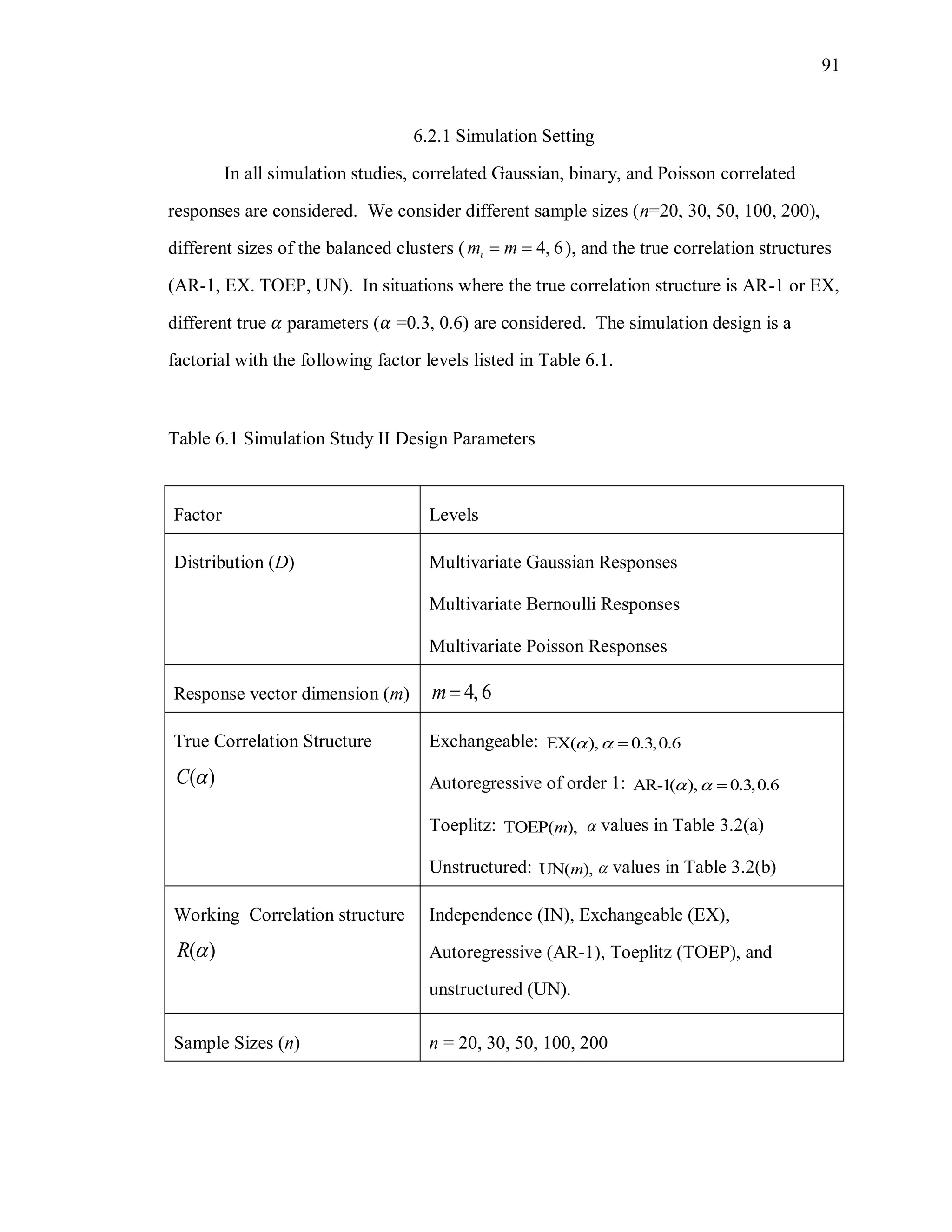
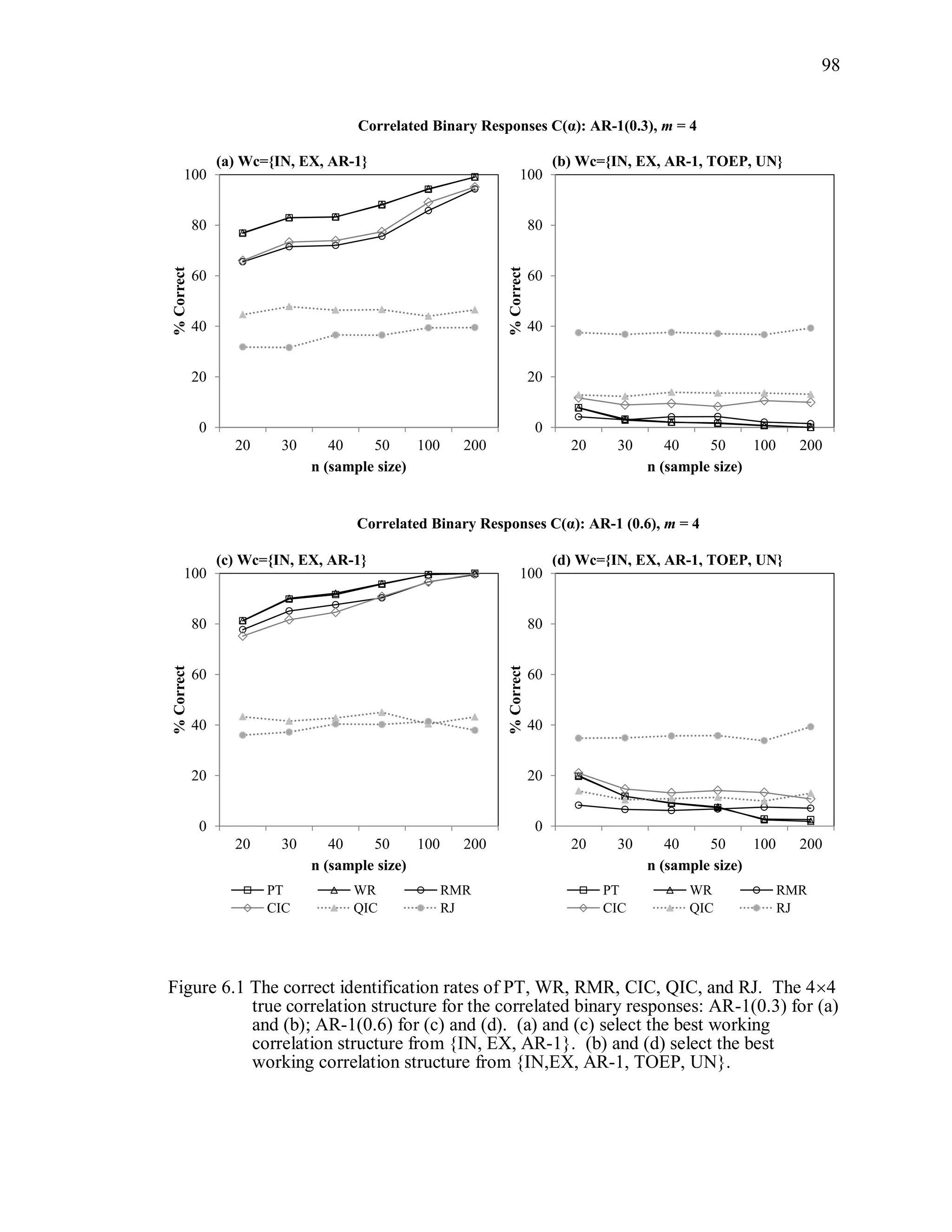
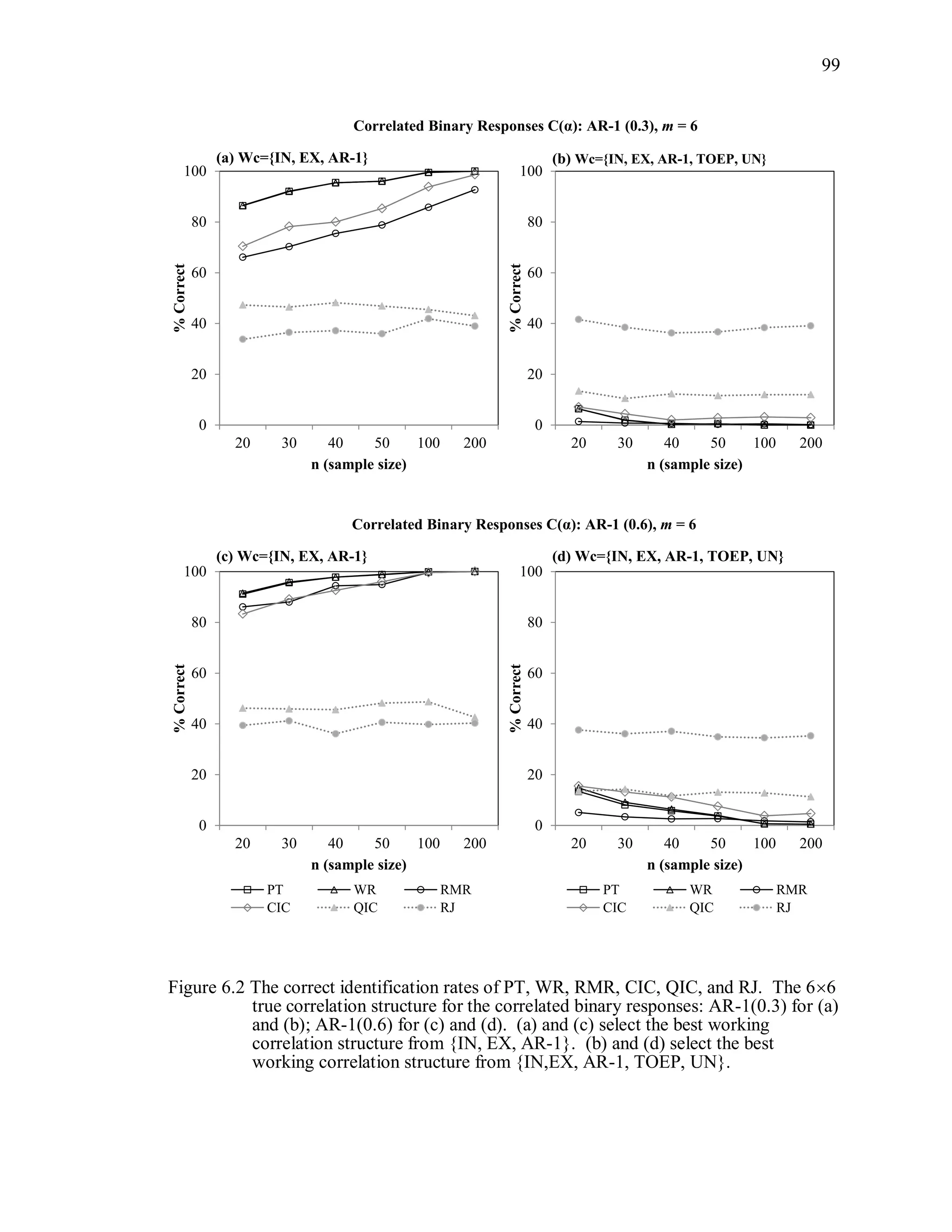
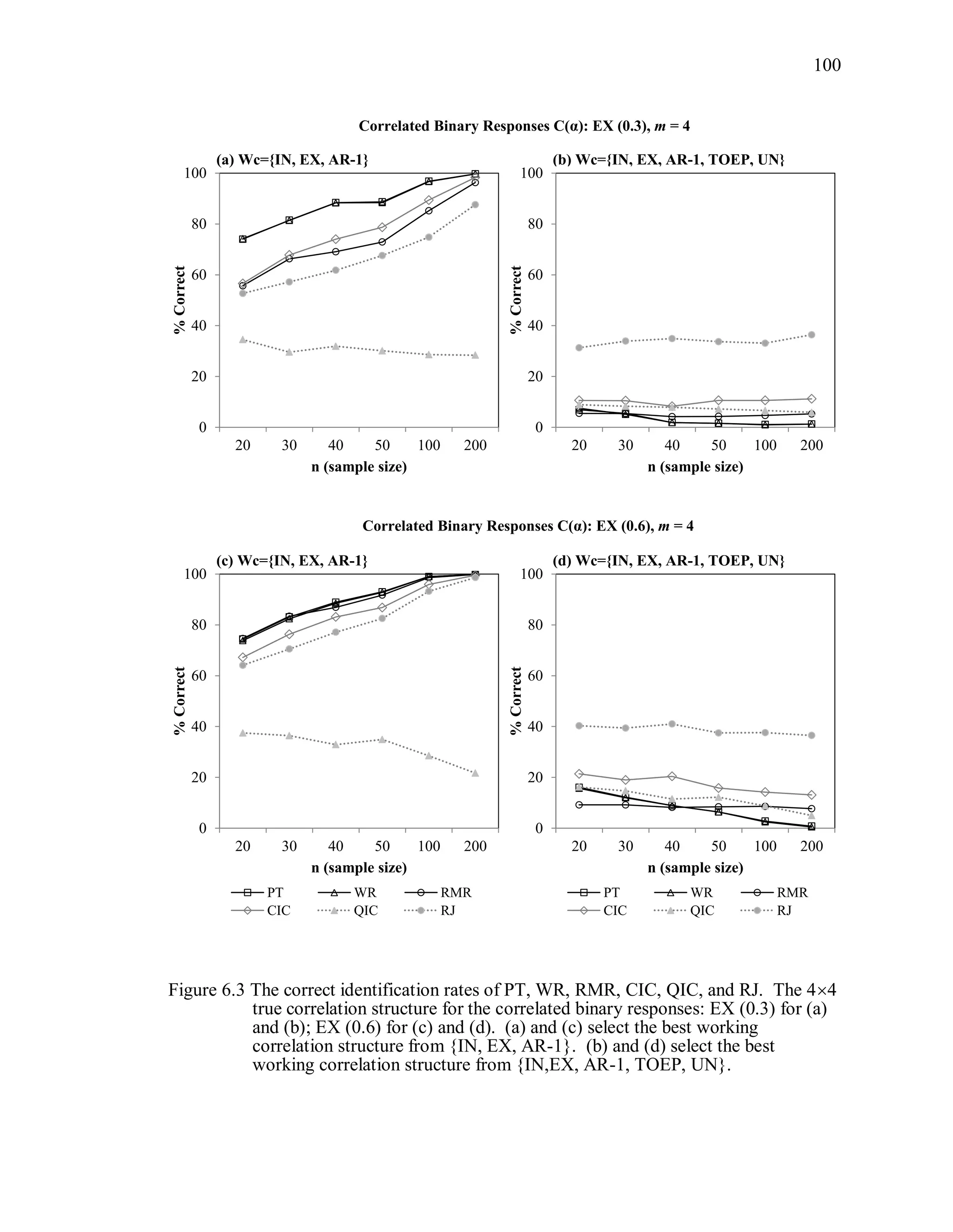
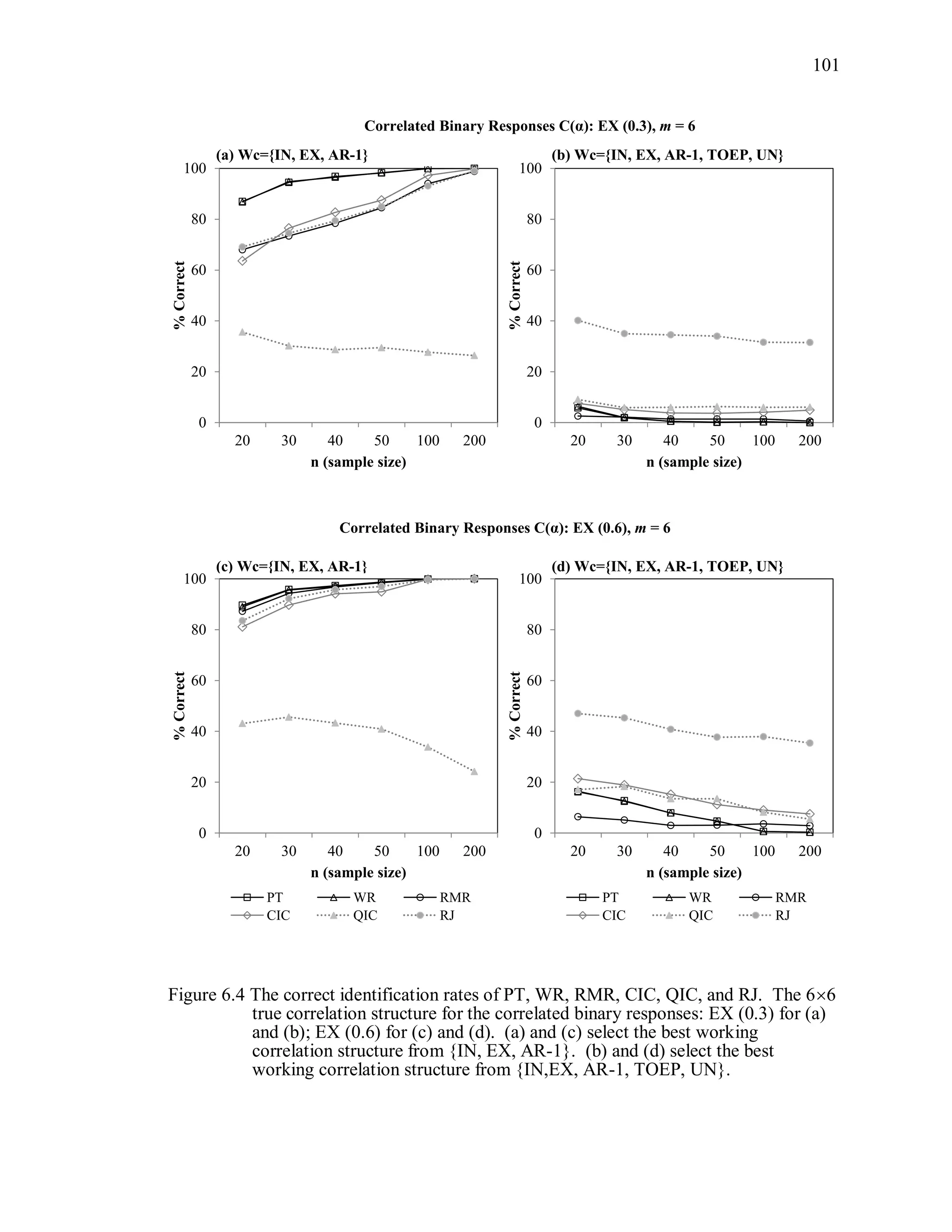
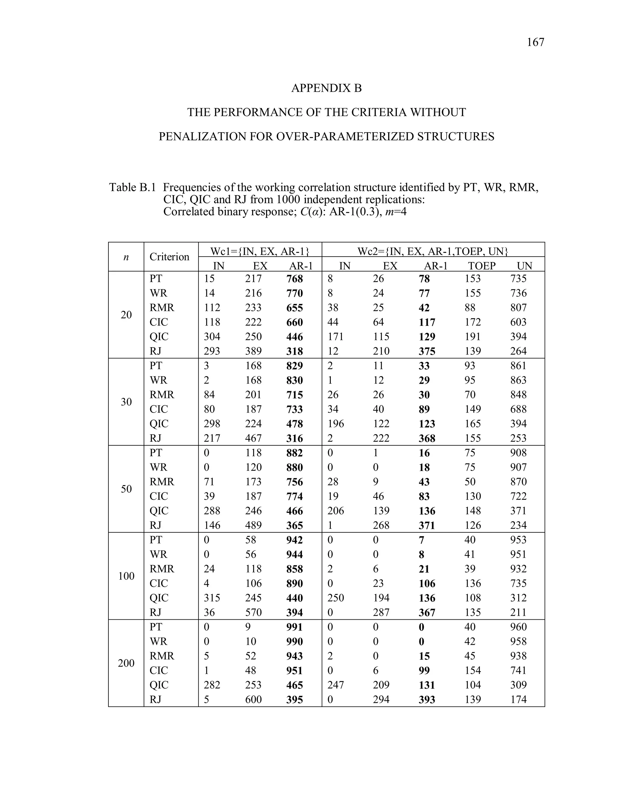
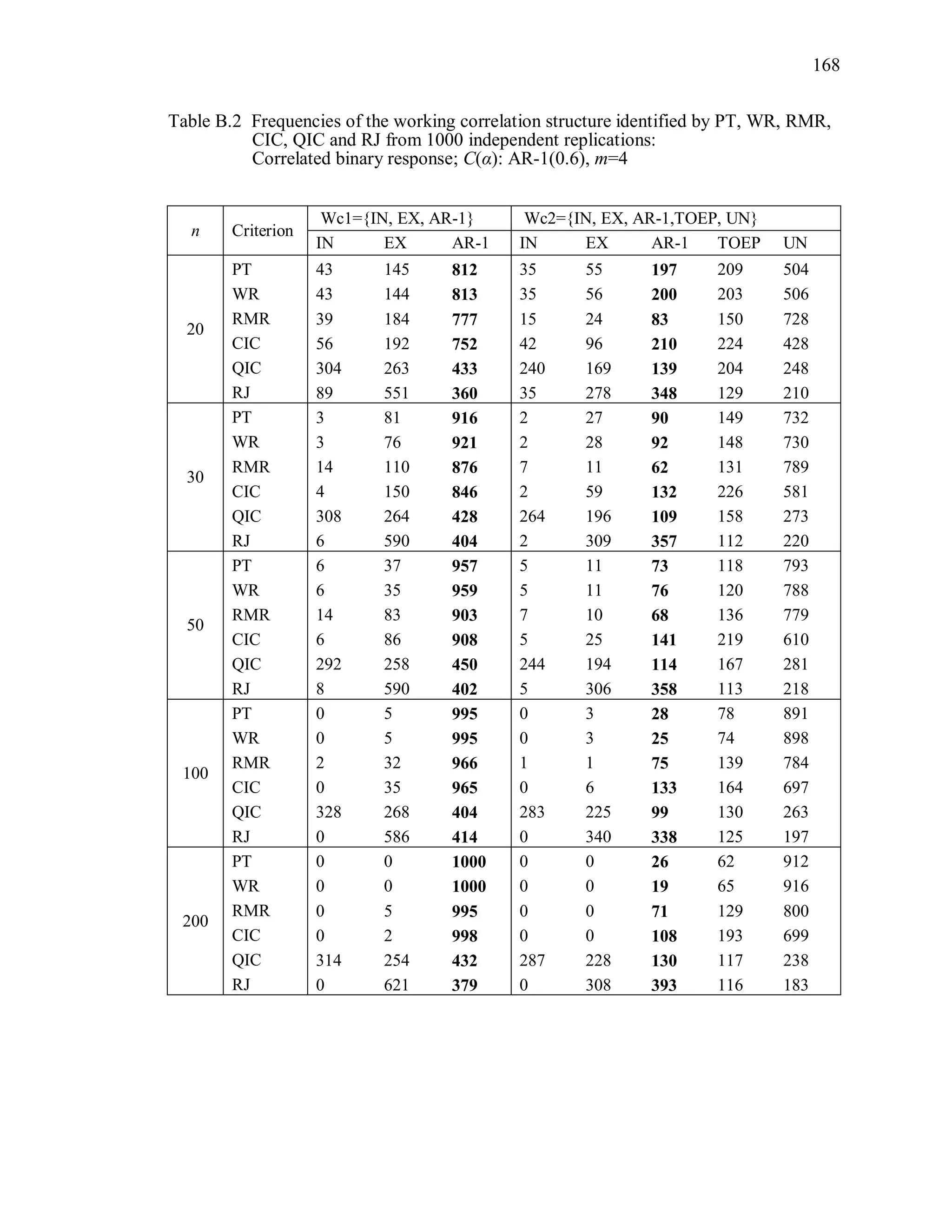
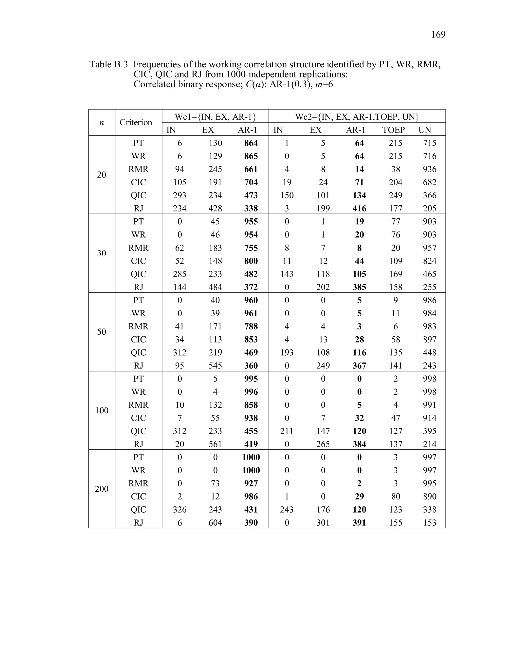
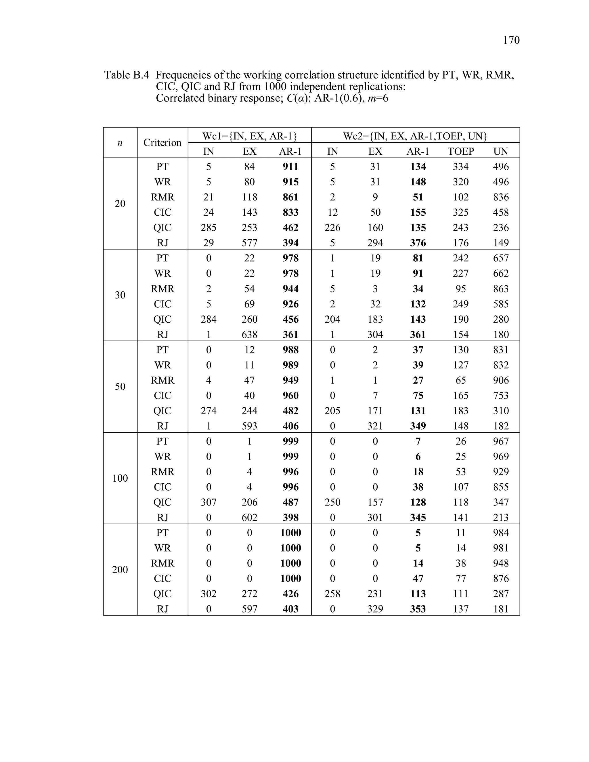
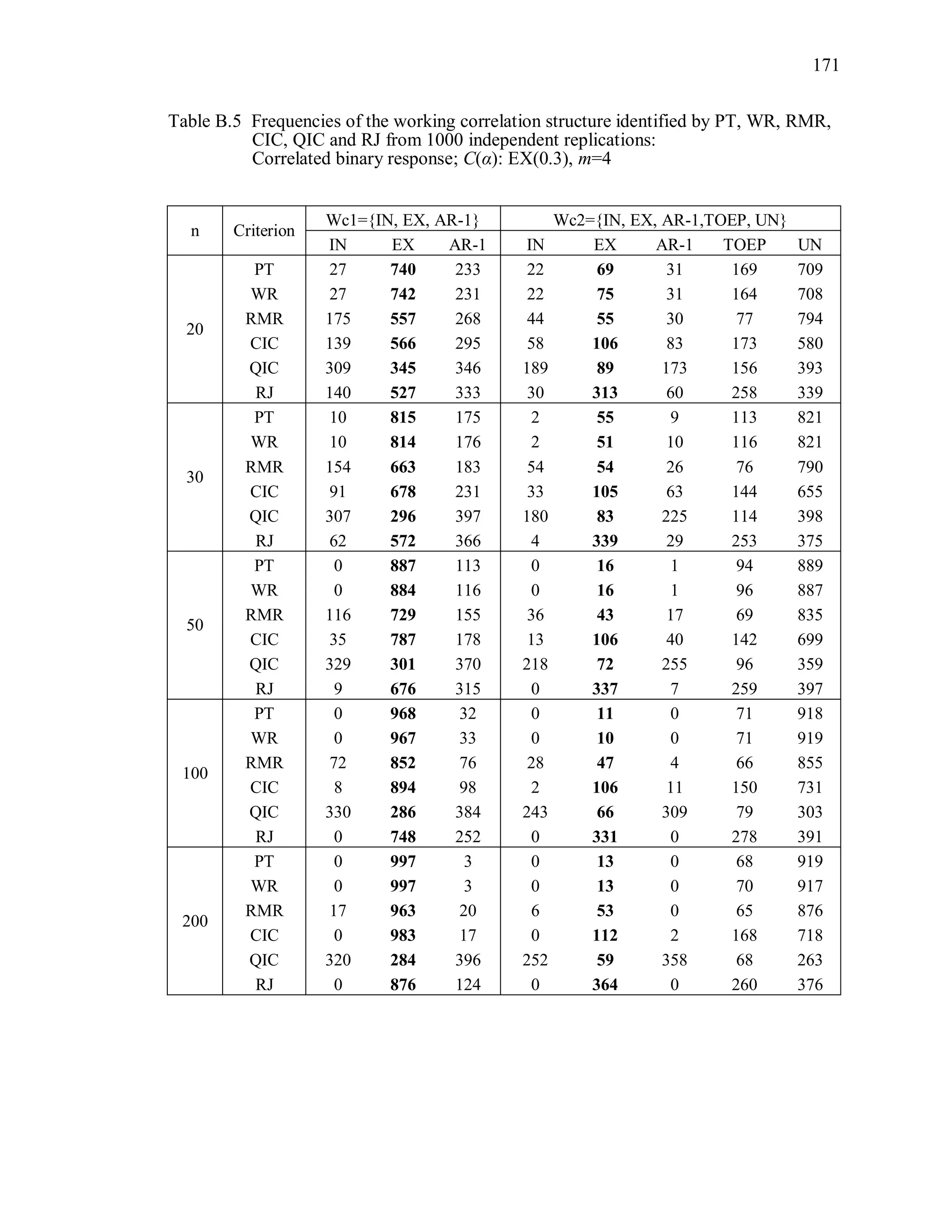
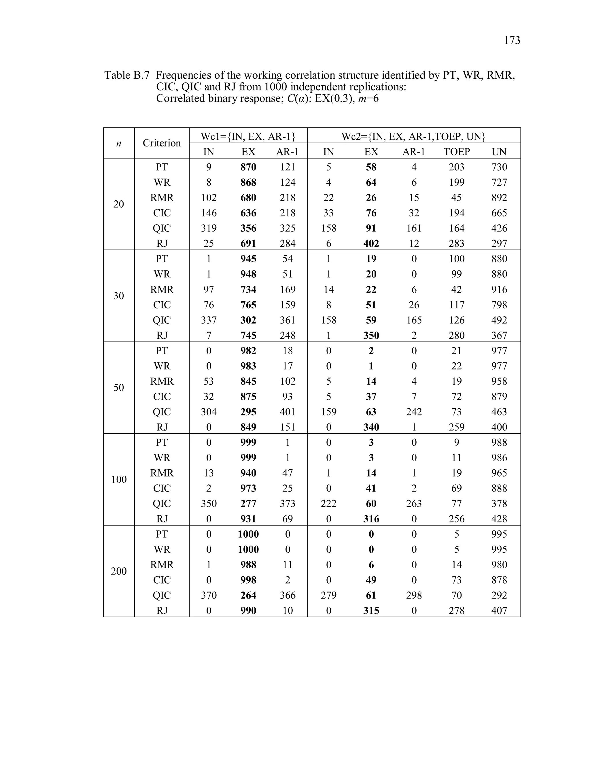
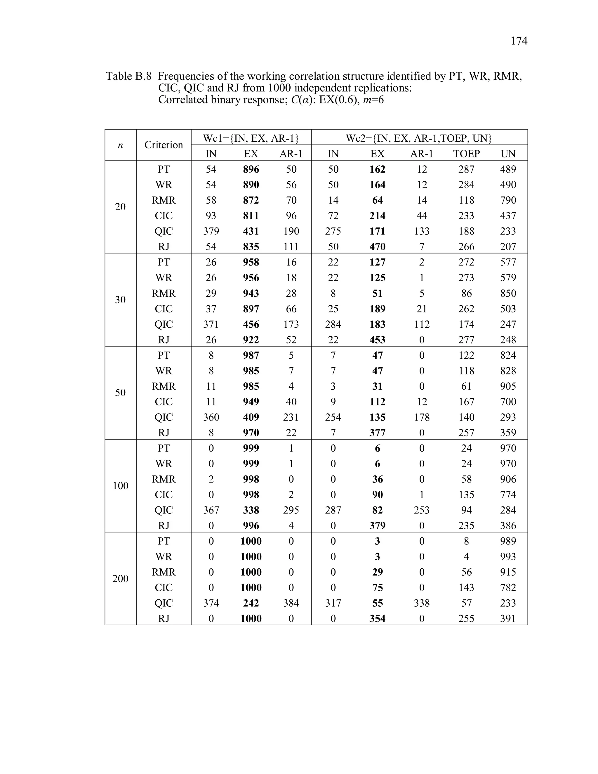
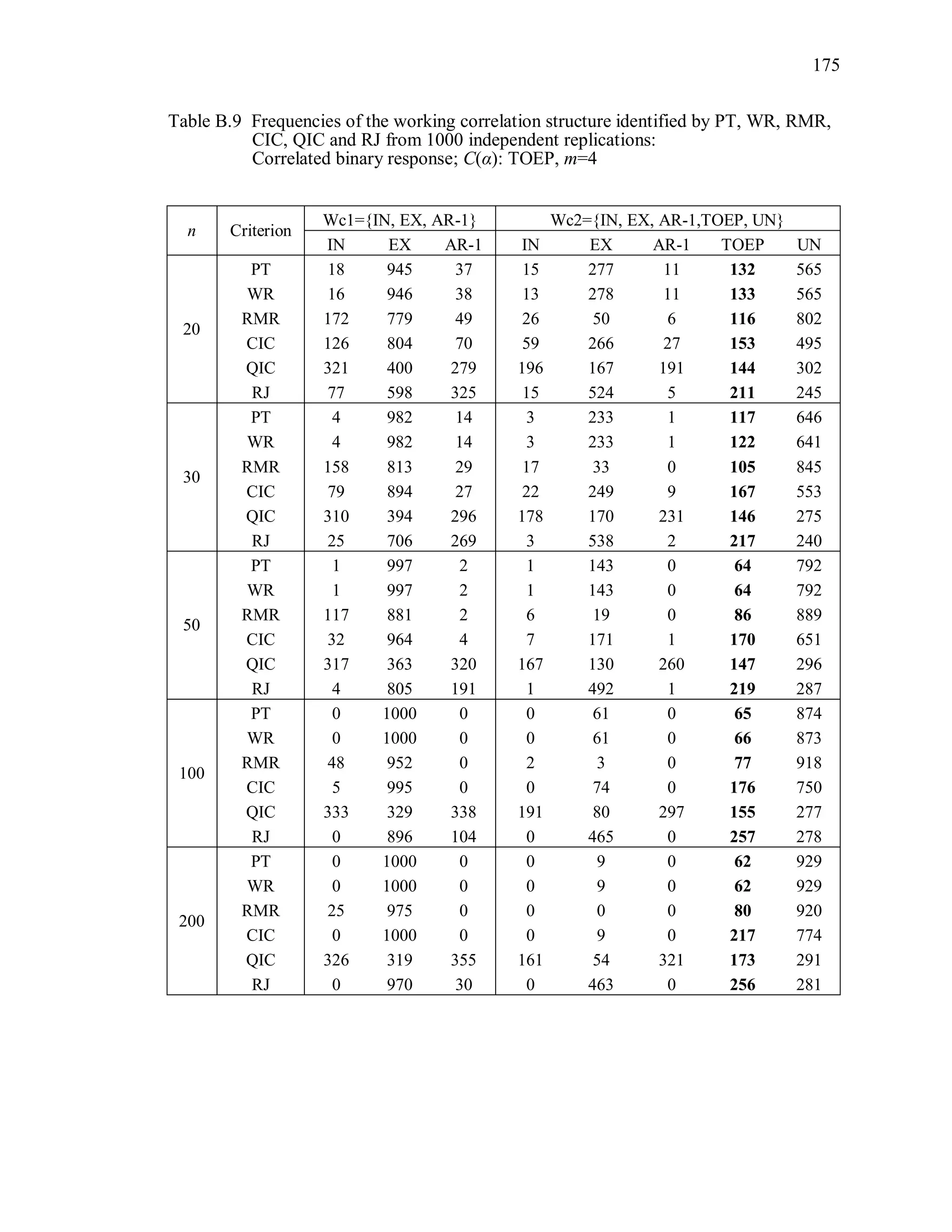
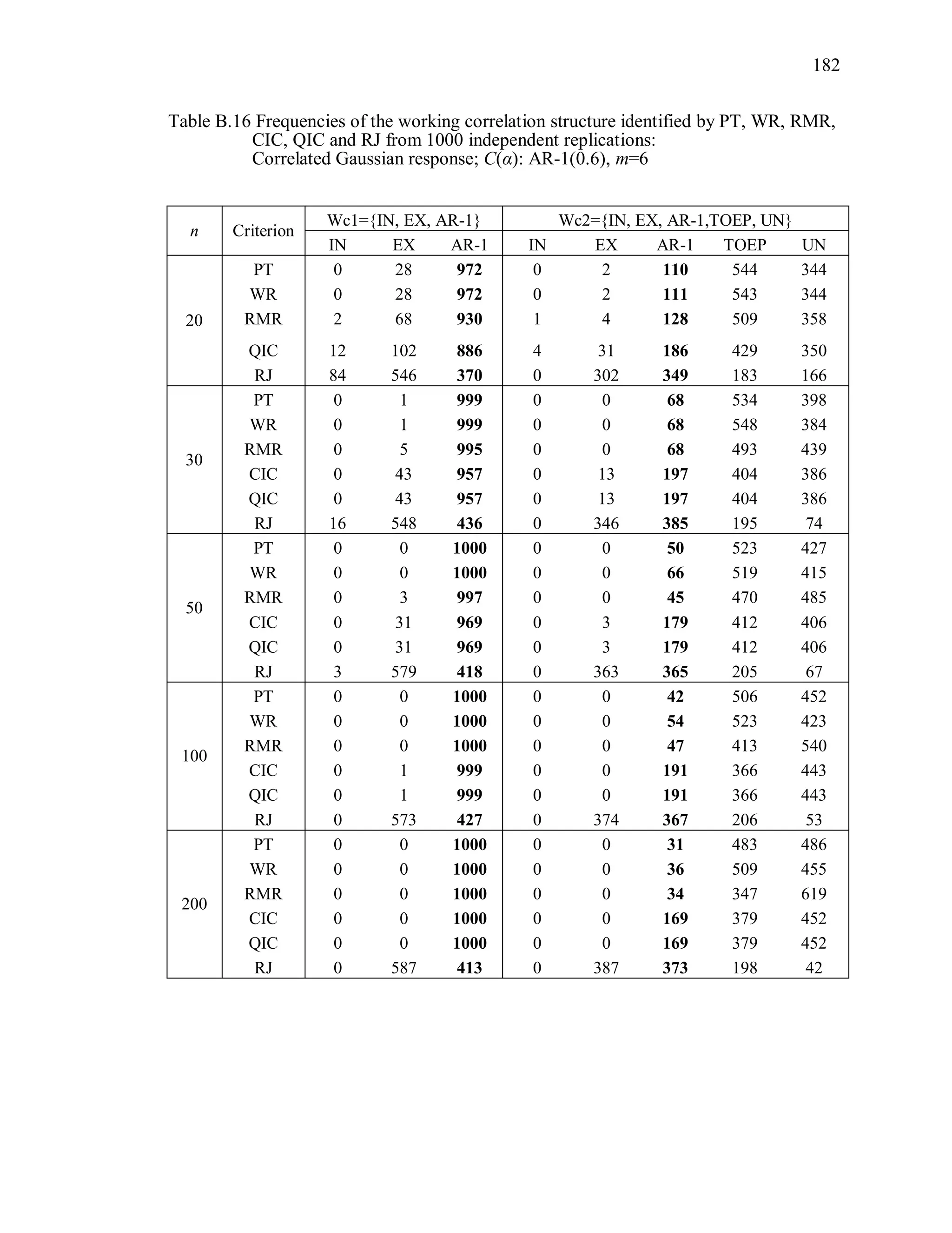
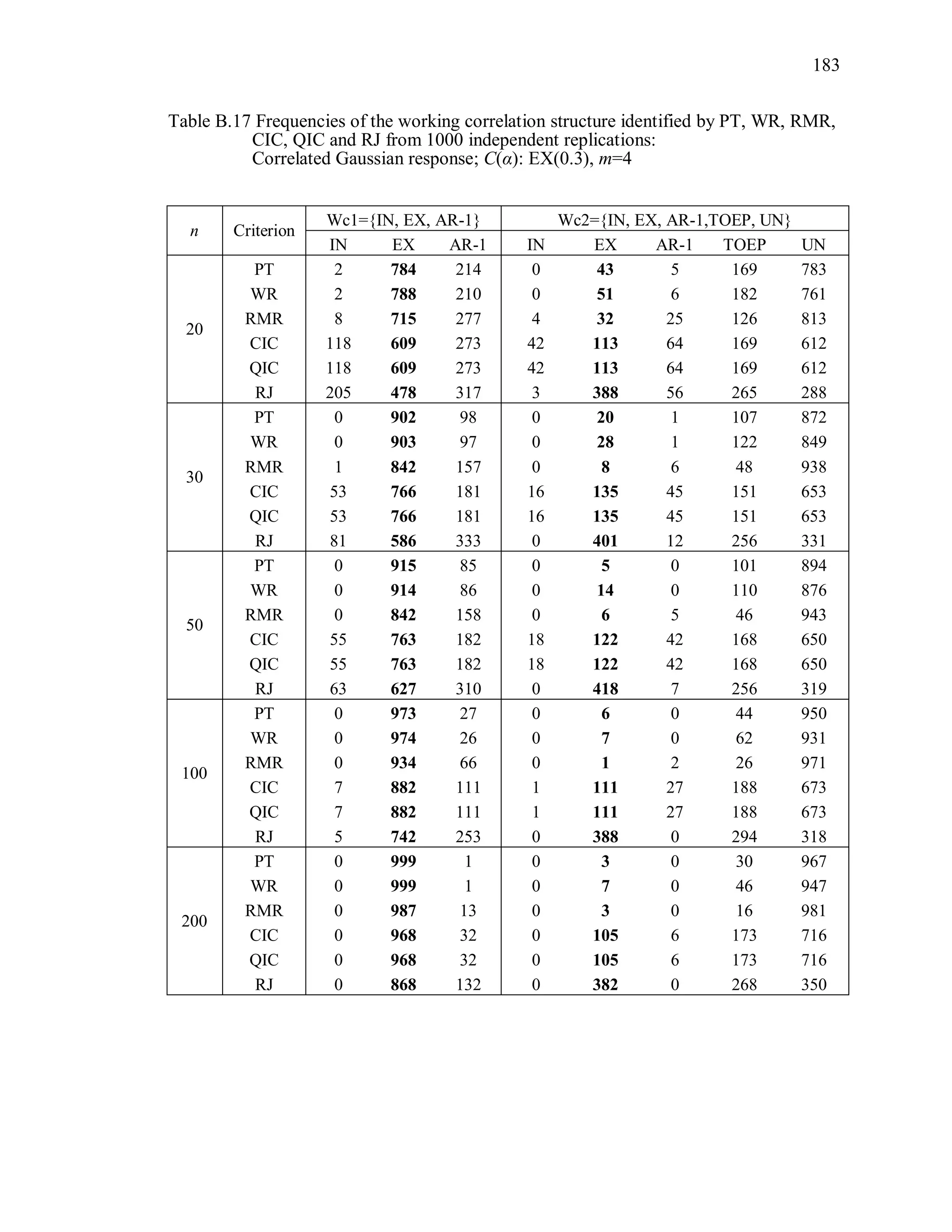
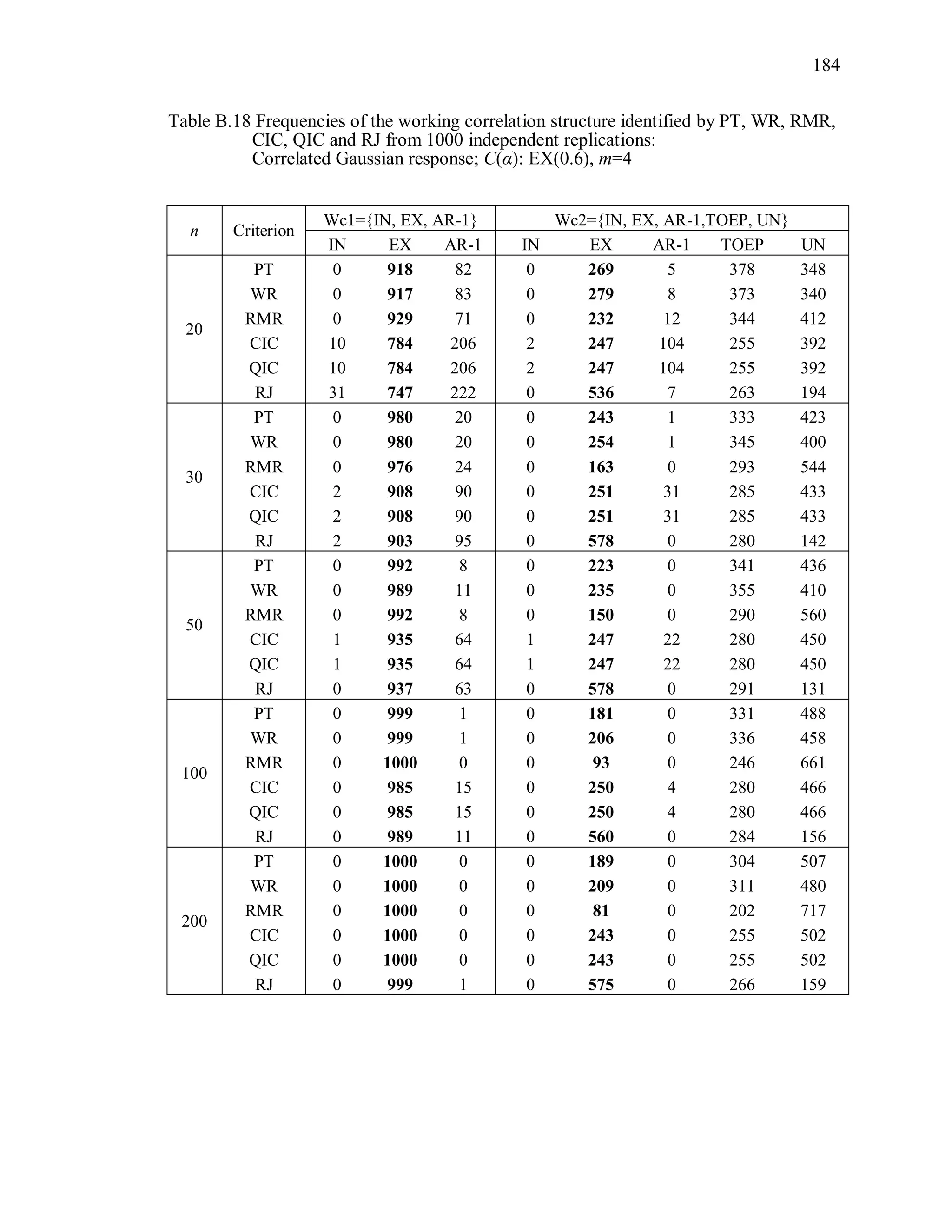
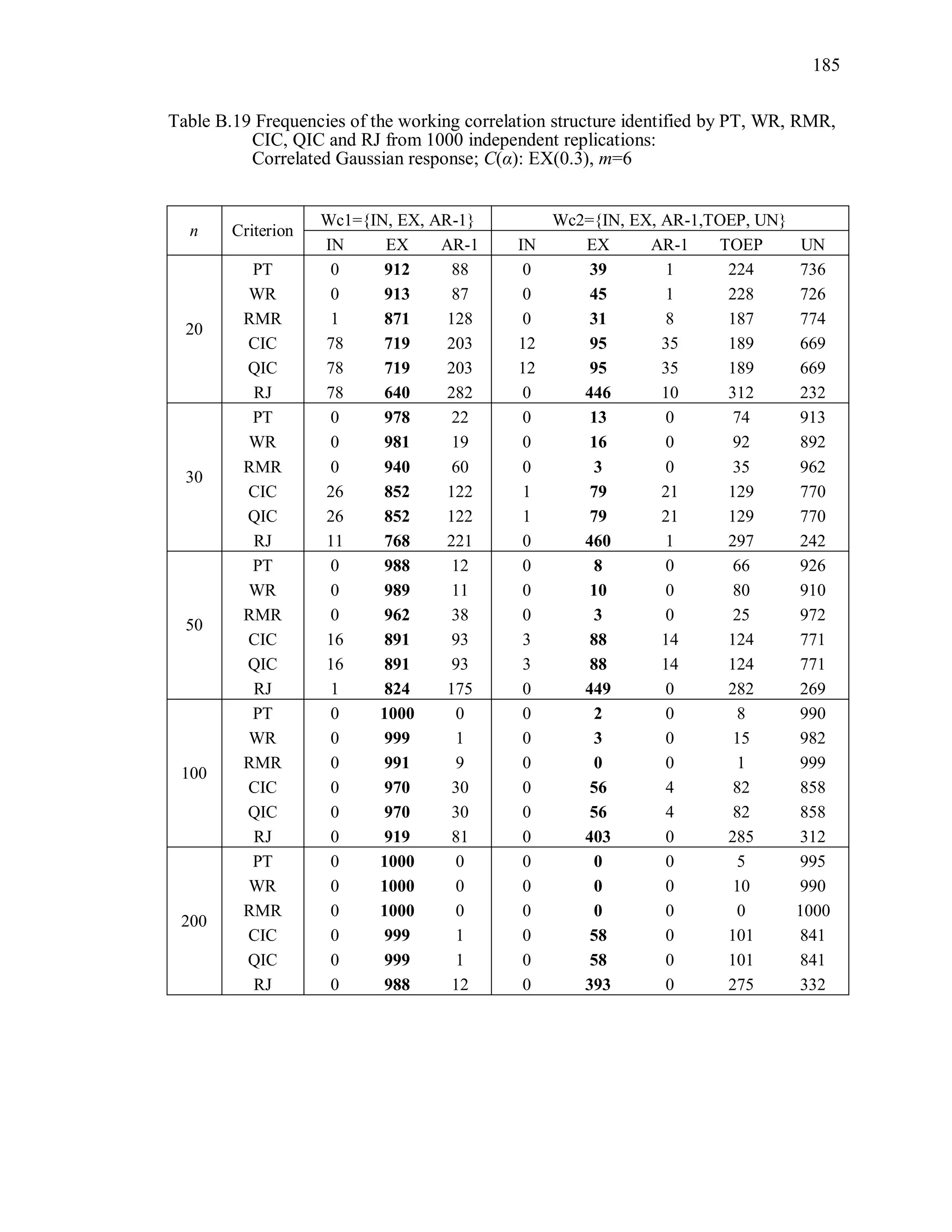
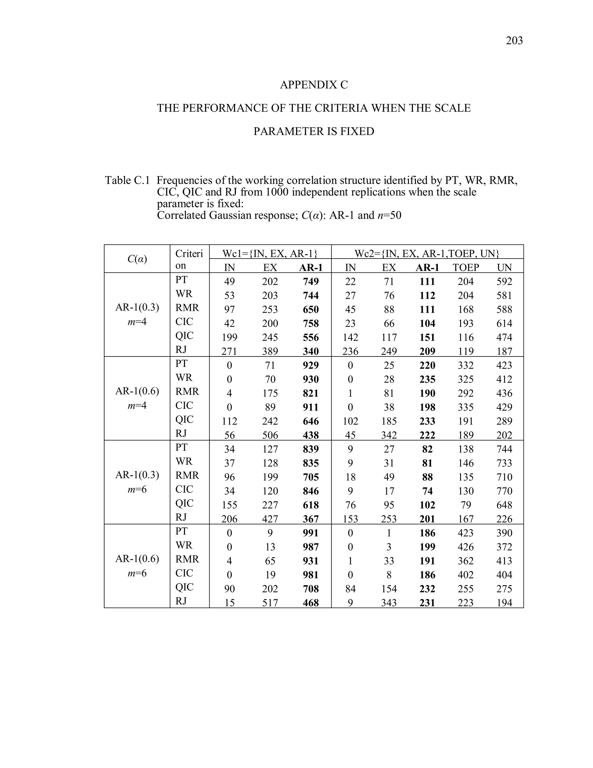
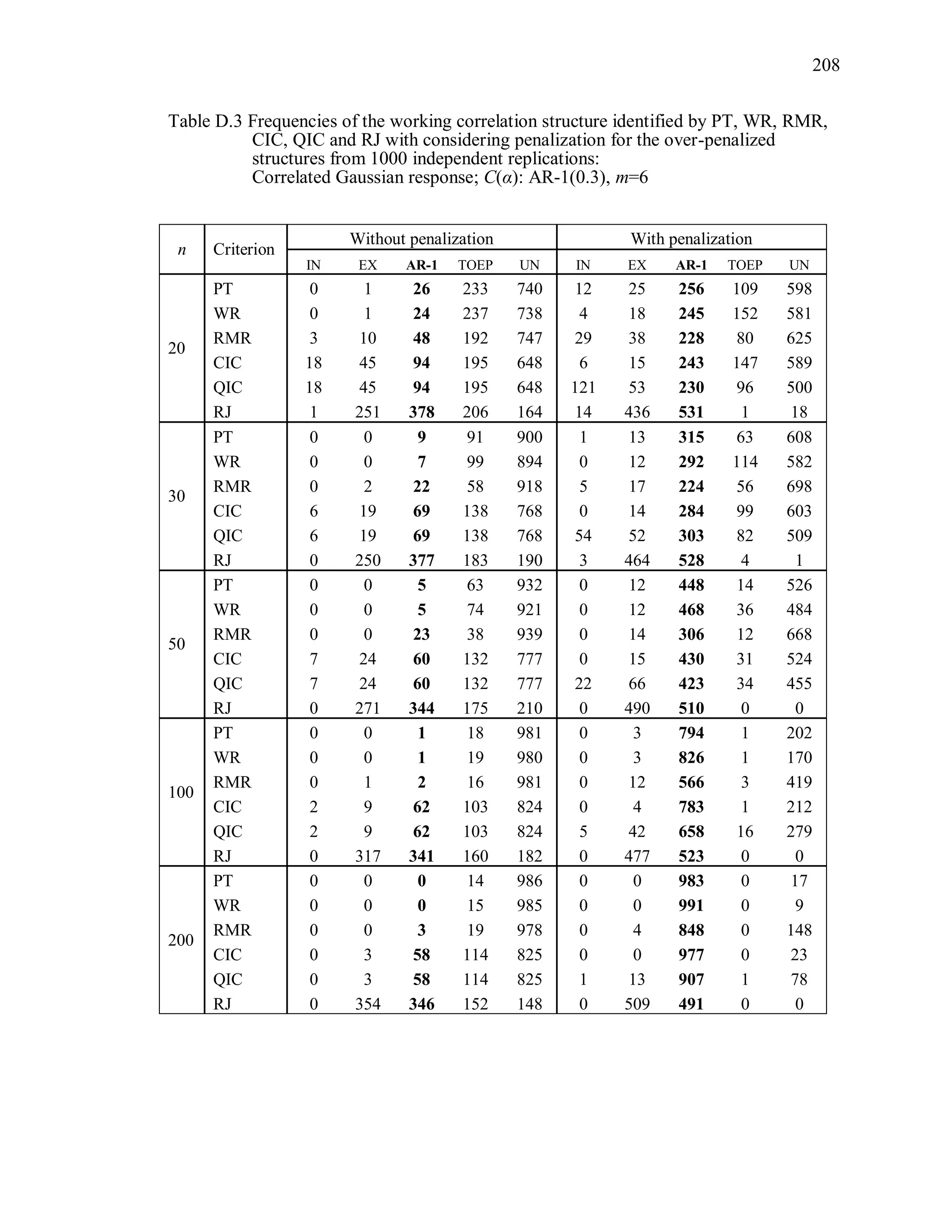
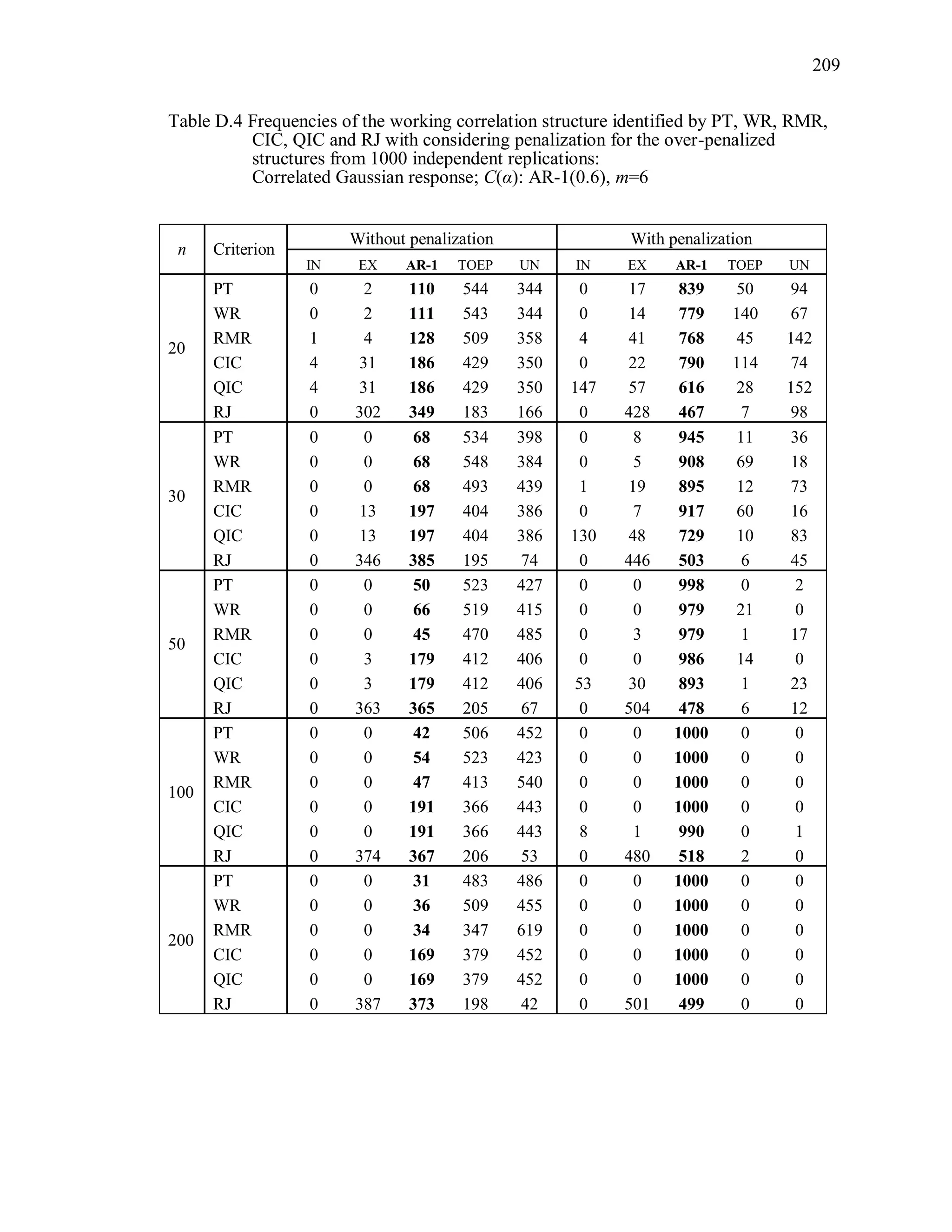
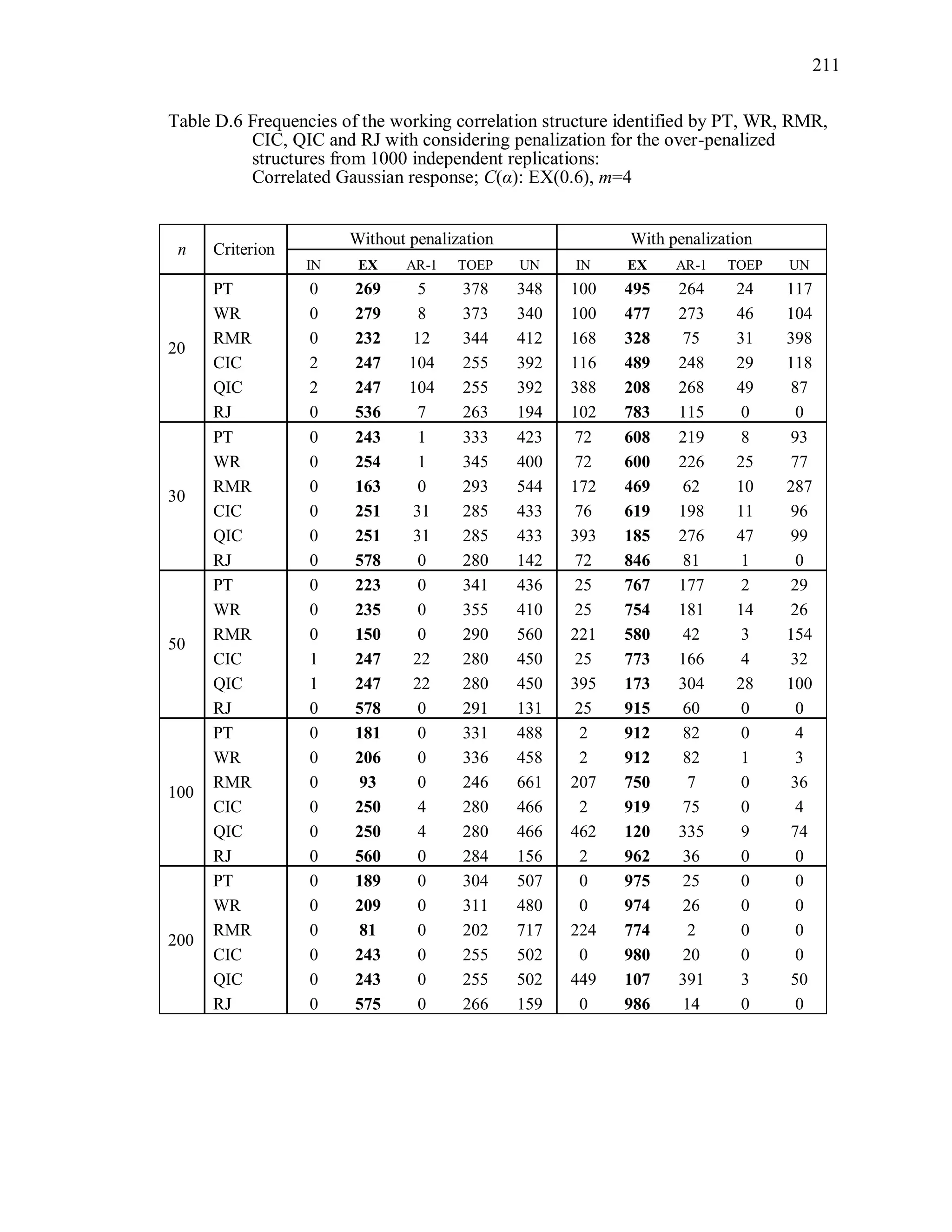
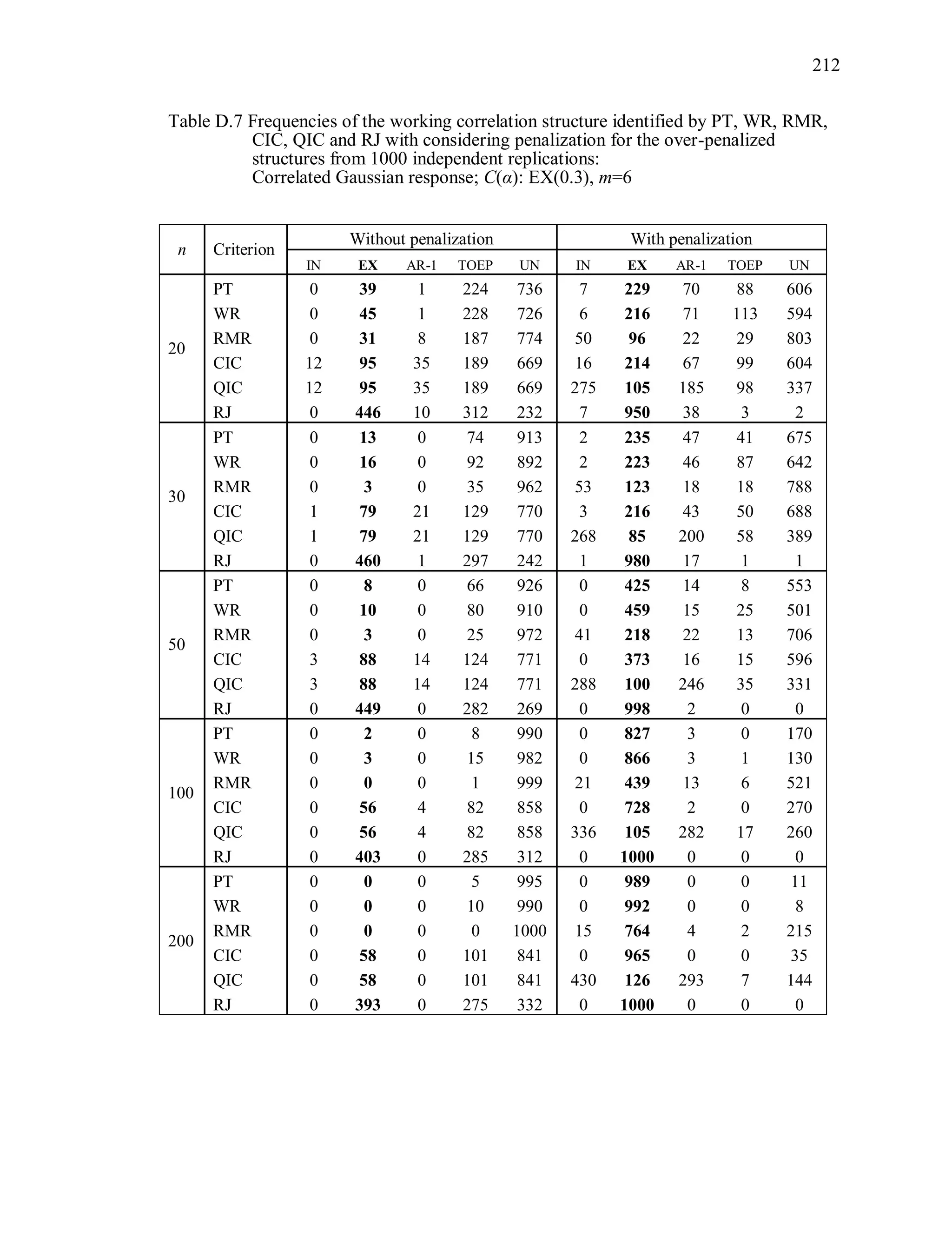
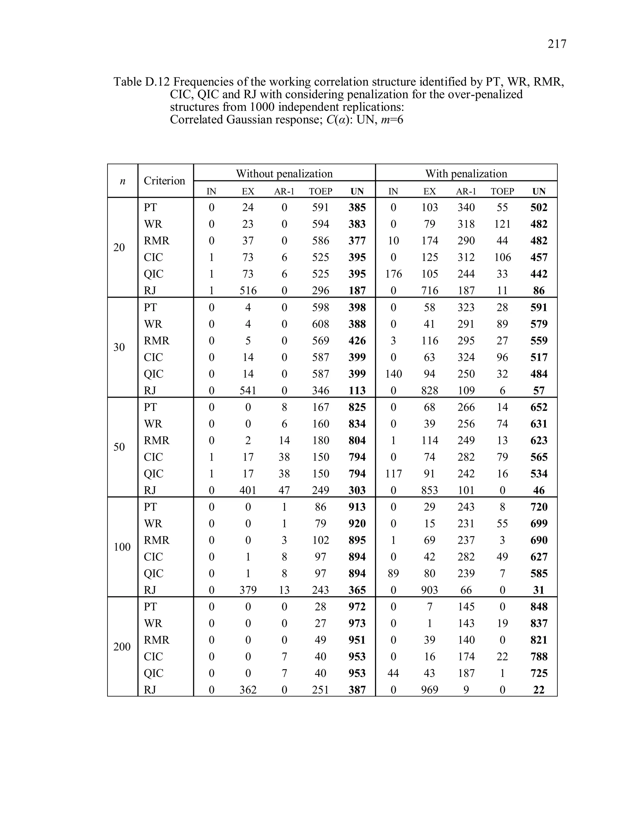
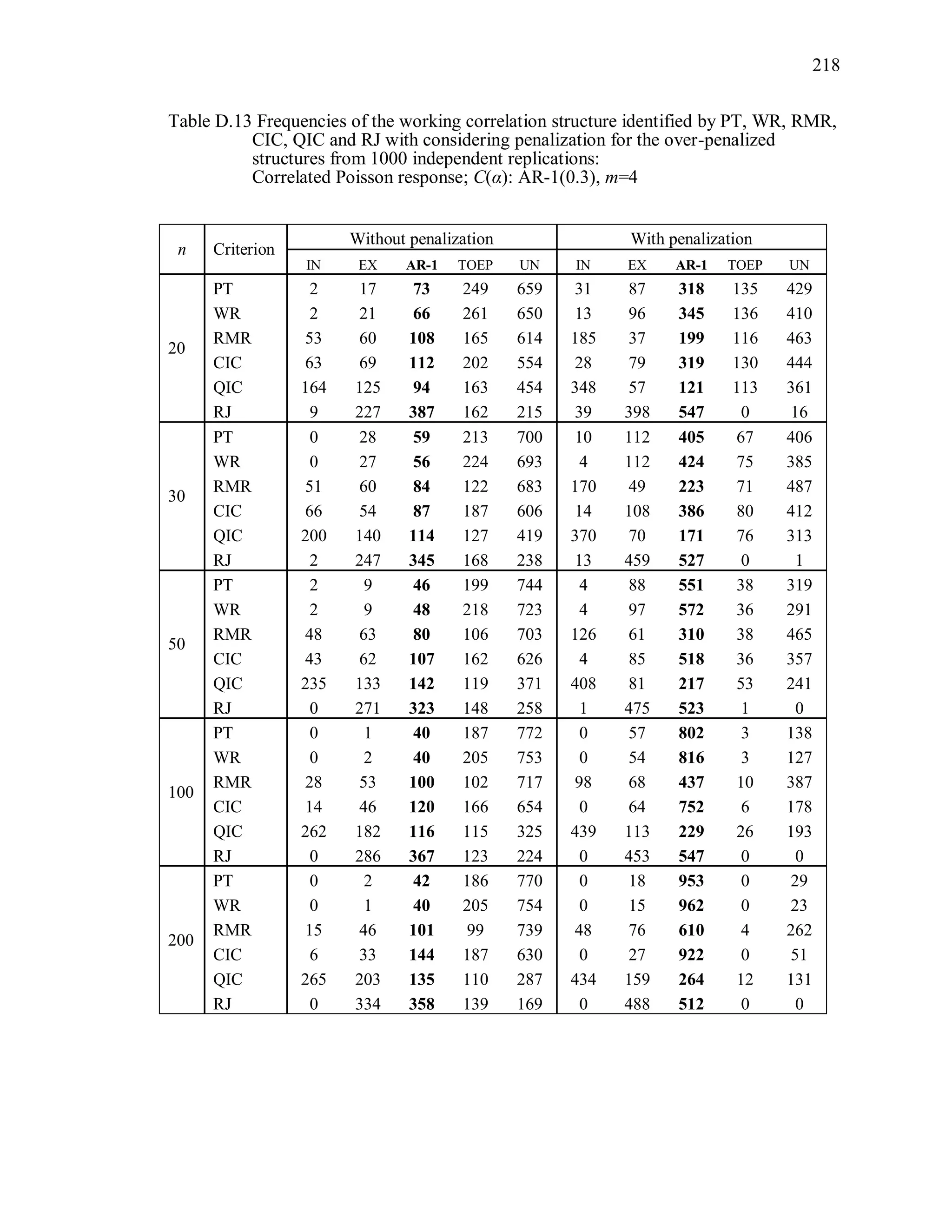
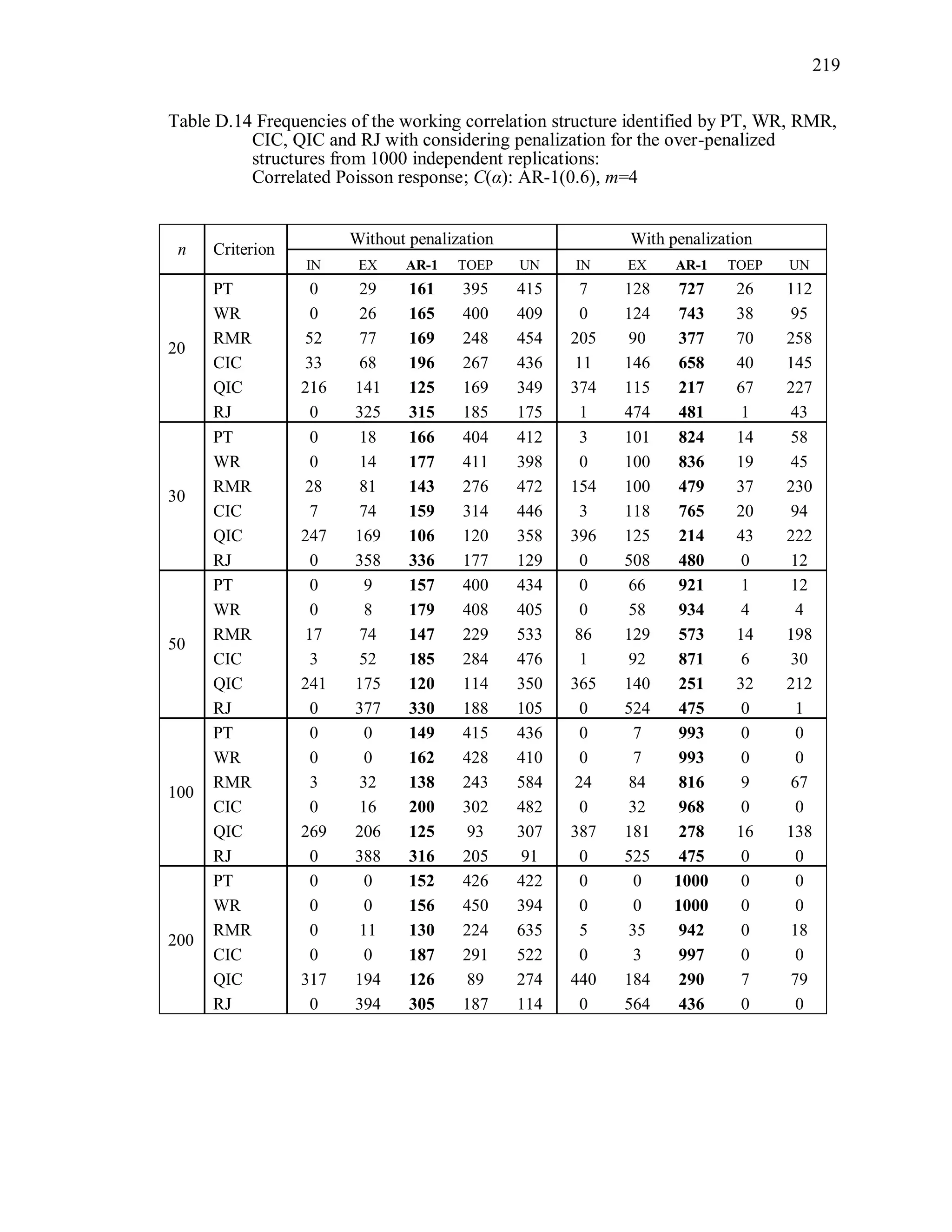
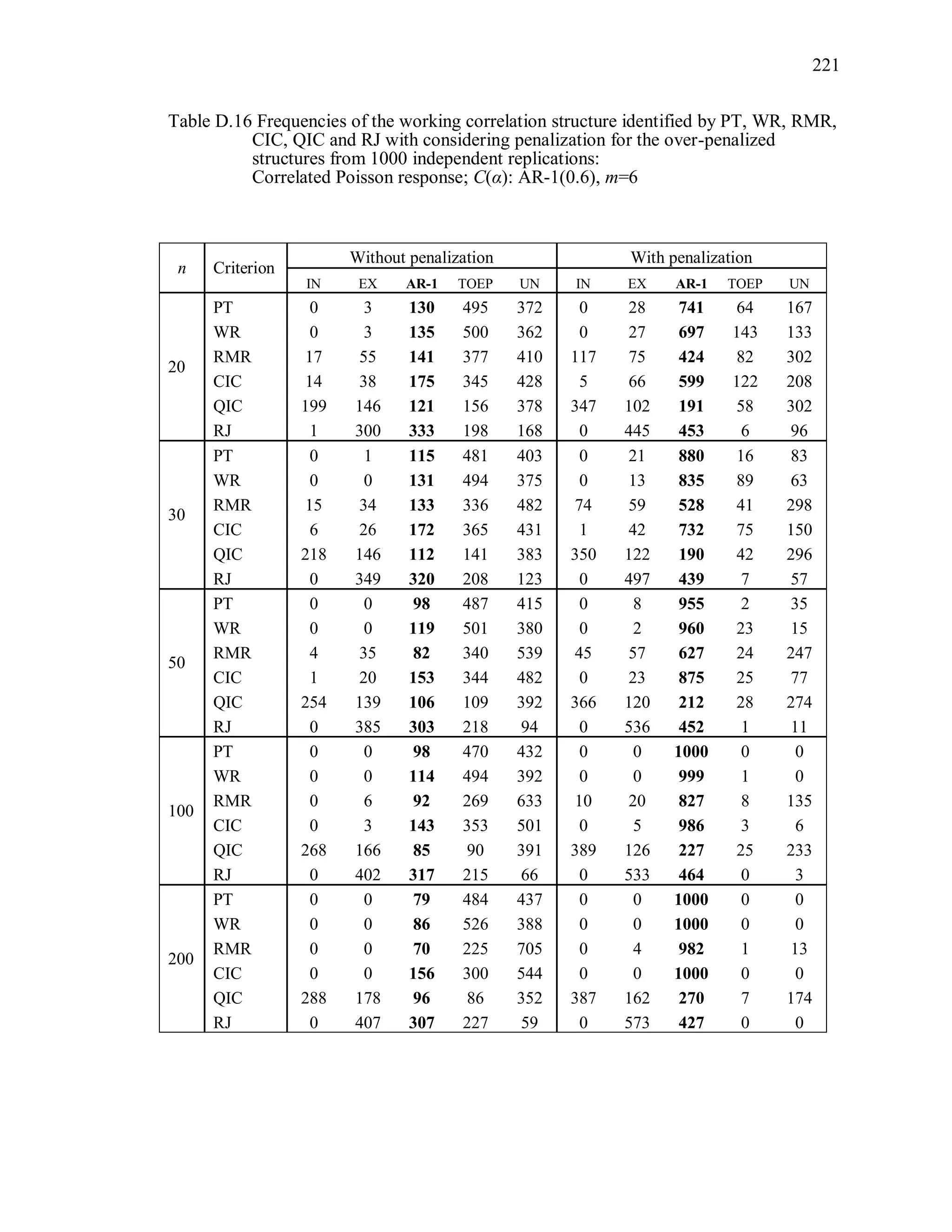
6.2 Simulation Study II
In the Simulation Study II, the new selection criteria for working correlation
structure (PT, WR and RMR) are compared with the existing selection criteria QIC, CIC,
and RJ in two different settings.
1. For each criterion, the best approximating working correlation structure is chosen
among independence, exchangeable and AR-1 only.
2. For each criterion, the best approximating working correlation structure is chosen
among independence, exchangeable, AR-1, Toeplitz and unstructured working
correlation structures.
The first setting allows a direct comparison to the comparable studies presented in the
literature, in which the competing working correlation structures have none or one 
parameter. The second reflects a more realistic setting in which overparameterized
candidate structures are included.

118. 91
6.2.1 Simulation Setting
In all simulation studies, correlated Gaussian, binary, and Poisson correlated
responses are considered. We consider different sample sizes (n=20, 30, 50, 100, 200),
different sizes of the balanced clusters ( 4, 6im m  ), and the true correlation structures
(AR-1, EX. TOEP, UN). In situations where the true correlation structure is AR-1 or EX,
different true parameters ( =0.3, 0.6) are considered. The simulation design is a
factorial with the following factor levels listed in Table 6.1.
Table 6.1 Simulation Study II Design Parameters
Factor Levels
Distribution (D) Multivariate Gaussian Responses
Multivariate Bernoulli Responses
Multivariate Poisson Responses
Response vector dimension (m) 4, 6m 
True Correlation Structure
( )C 
Exchangeable: EX( ), 0.3,0.6 
Autoregressive of order 1: AR-1( ), 0.3,0.6 
Toeplitz: TOEP( ),m  values in Table 3.2(a)
Unstructured: UN( ),m  values in Table 3.2(b)
Working Correlation structure
( )R 
Independence (IN), Exchangeable (EX),
Autoregressive (AR-1), Toeplitz (TOEP), and
unstructured (UN).
Sample Sizes (n) n = 20, 30, 50, 100, 200

119. 92
The marginal mean of the t-th component of the correlated Gaussian response
vector iy is 1 1 2 2( )it it t tE y x x     , where 1 2 0.3   , the true scale parameter
1,T  1tx and 2tx are independently generated from [0,1]U . This is the same marginal
mean model used by Hin and Wang (2009). For the correlated binary responses, the
components of the mean vector are modeled as 1 1 2 2logit( ) ,it t tx x    where 1tx and
2tx are independently generated from [0.5,1]U and 1 2 0.3   . For correlated Poisson
responses, the components of the mean vector are modeled as 1 1 2 2log( ) ,it t tx x   
where 1tx and 2tx are independently generated from [0.5,1]U and 1 2 0.3   . For all
simulations, 1tx and 2tx are observational-level covariates.
All correlation/covariance matrices used in the simulation are positive definite,
and the same covariance structures are used for the m-dimensional Gaussian, multivariate
Bernoulli, and multivariate Poisson random vectors. For the correlated binary responses,
the marginal means limit the ranges of the correlations (Qaqish, 2003). The correlation
coefficients (i.e.,  parameters) of the true Toeplitz and unstructured matrices presented
in Table 3.2 were chosen so that they satisfied the correlation bounds for the binary
responses, as well as being proper pairwise correlations for the Poisson and Gaussian
distributions.
A sample of n independent simulated observations with response vector of size m,
true correlation structure C(α), and distribution D are generated under the marginal mean
and true correlation structure. The model is fit under the correct marginal mean model
and the correct variance function, but assuming each of five different working correlation
structures (R(α)=IN, EX, AR-1, TOEP, UN) and using that one data set. This is
replicated r = 1000 times.
Working correlation selection criterion measures are computed using the bias-
corrected sandwich variance estimator by Wong and Long (WL), which was not the
original proposed structure of QIC or CIC. As shown in Simulation Study I, the WL
variance estimator effectively corrects the negative bias of the Liang and Zeger’s

120. 93
sandwich variance estimator and tends to have smaller variability in small samples than
other sandwich variance estimators. Thus, it appeared to be the best choice for this
investigation, so as not to confound issues of bias with issues of working correlation
selection.
Each selection criterion selects the best approximating working correlation
structure within the listed set of five candidate structures. Through 1000 independent
simulation replications, the performance of each criterion is determined based on the
frequency of choosing the correct structure out of 1000.
All simulations are performed using R version 2.11.1. Correlated Gaussian
random variables are generated using the MASS library, and correlated binary data are
generated using the binarySimCLF library (Qaqish, 2003). For every mean vector and
correlation matrix based on correlated binary responses, conditional linear family (CLF)
compatibility is checked. As defined in Qaqish (2003), the conditional linear family is a
subset of all multivariate binary distributions, and used in this algorithm for efficiently
generating large multivariate vectors with specified marginal probabilities and correlation
matrices. If a single observation ( ,i iY X ) simulated data does not meet the CLF
compatibility criterion, it is discarded and a new independent correlated binary random
vector is generated. Correlated Poisson random variables are generated using the method
proposed by Yahav and Shmueli (2011). Generating random vectors in this manner is
repeated until 1000 samples of size n are obtained. The GEE fitting within R is
performed using the geese( ) function in the geepack package.
6.2.2 Simulation Results: Correlated Binary Response
Figure 6.1 through Figure 6.4 present the correct identification rates of the six
criteria (PT, WR, RMR, CIC, QIC, RJ) for the correlated binary responses under the
different true correlation structures. In particular, the frequencies of the working
correlation structure identified by the six criteria when n=50 and m=4 are tabulated in

121. 94
Table 6.2. Simulation results for the correlated Gaussian and Poisson responses also
present similar results, so their results are not shown here, but are included in Appendix
B.
The correct identification rate for each criterion is defined as the percent of
selecting the true correlation structure out of 1000 independent simulations. For a given
simulated data set (i.e., one replication of the simulation), the best working correlation
structure is selected from two sets of the candidate structures 1Wc ={IN, EX, AR-1} and
2Wc ={IN, EX, AR-1, TOEP, UN} separately.
If the true correlation structure ( )C  is included in 1Wc ={IN, EX, AR-1} and
TOEP and UN are not considered as candidates, PT, WR, and CIC select the correctly-
specified working correlation structure with high rates. RMR performs a little bit worse.
This is probably because RMR uses only the largest generalized eigenvalue whereas PT,
WR, CIC utilize all generalized eigenvalues to measure the discrepancy between two
covariance matrices. If AR-1 is the true correlation structure, QIC and RJ are poor at
identifying the correct structure as compared to PT, WR and CIC (Figure 6.1(a)(c) and
Figure 6.2(a)(c)). On the contrary, if EX is the true correlation structure, RJ performs
very similarly to PT, WR, and CIC in selecting the correct structure (Figure 6.3(a)(c) and
Figure 6.4(a)(c)).
If 2Wc is {IN, EX, AR-1, TOEP, UN} and the true correlation structure is any
patterned matrix, all six criteria perform poorly. Overall, PT, WR, CIC, and RMR prefer
the unstructured working correlation structure, reflecting the ability of that structure to fit
to any dataset (Table 6.2). They rarely choose the incorrect under-parameterized
structures (i.e., misspecified structures). For instance, if the true correlation structure is
AR-1, they rarely select IN or EX. On the other hand, QIC and RJ select the misspecified
structures approximately 30% of the time. Independent working correlation structure is
sometimes chosen by QIC, whereas other criterion measures hardly ever select it.
Exchangeable working correlation is preferred by RJ for most cases. The RJ criterion, as

122. 95
designed, chooses the working correlation structure where the sandwich variance
estimate is nearest to the model-based variance estimate. The simulation results show
that RJ tends to select the exchangeable structure regardless of the true underlying
correlation structure, which is also shown in Hin et al. (2007). RJ seems to perform better
than other criterion measures when 2Wc ={IN, EX, AR-1, TOEP, UN}, but its correct
identification rate is still below 50%.
In summary, the proposed selection criteria, as well as CIC, perform similarly
well when the true correlation structure is parsimonious and a set of candidate structures
does not contain any over-parameterized structures. However, they tend to select an
over-parameterized working correlation structure much of the time – with QIC doing so
less often because it is choosing independence structure. The unstructured, and to a
lesser extent, the Toeplitz working correlation structures are more likely to be selected by
those criterion measures. Since the unstructured matrix closely approximates the true
correlation structure in large samples, the loss of statistical efficiency of ˆ would be
trivial in that case. However, in small to moderate sample sizes, the use of the
unstructured matrix causes the hypothesis testing to be liberal, as shown in chapter 2.
6.2.3 Simulation Results: Correlated Gaussian Response
When the response vector is the correlated Gaussian response, the similar patterns
are identified (Table B.13 ~ Table B.24 in Appendix B). Note that both QIC and CIC
select the same working correlation structure all the time for the correlated normal
responses if the scale parameter is estimated for each different model. When the scale
parameter is estimated for each different model, QIC becomes ( ) 2CICN p  for the
correlated normal responses where N=nm and p is the dimension of ˆ . Since ( )N p
is the constant, QIC and CIC select the same working correlation structure. Hin and
Wang (2009) fixed scale parameter in their simulations and showed the superiority of

123. 96
CIC over QIC for working correlation selection. It is worth to evaluate the effect of fixed
scale parameter on the performance of the criterion measures. Except QIC, the
performance of other criterion measures are found to be hardly influenced by the fixed
scale parameter as compared to simulation results when the scale parameter is estimated.
On the other hand, QIC performs worse than PT, WR, and CIC when the scale parameter
is fixed (Tables C.1 ~ C.4 in Appendix C). In practice, the true scale parameter is
unknown. Regression parameter estimates and covariance estimates based on the
estimated scale parameter are used for inference. Moreover, it was shown that other
criterion measures which are superior to QIC were little impacted by whether or not scale
parameter is fixed. Therefore, for the rest of this paper, simulation results when the scale
parameter is estimated differently in each candidate models will be shown.
6.2.4 Simulation Results: Correlated Poisson Response
When the response vector is the correlated Poisson response, the similar patterns
are identified (Table B.25 ~ Table B.36 in Appendix B). When the over-parameterized
structure is included (i.e., 2Wc ={IN, EX, AR-1, TOEP, UN}) and the true underlying
correlation structure is parsimonious such as AR-1 or exchangeable, all six criteria tend
to select the over-parameterized structure.
Therefore, penalization for over-parameterized structure is required to improve
the performance of the proposed selection criteria in small samples. In the next chapter, a
new method for penalizing over-parameterized structure is introduced.

124. 97
Table 6.2 Frequencies of the working correlation structure identified by PT, WR, RMR,
CIC, QIC, and RJ from 1000 independent replications. The true correlation
structures for the correlated binary responses are AR-1 (α = 0.3, 0.6) and
EX(α = 0.3, 0.6), m = 4 and n = 50.
( )C  Criterion
Wc ={IN, EX, AR-1} Wc ={IN, EX, AR-1, TOEP, UN}
IN EX AR IN EX AR TOEP UN
AR-1(0.3)
m = 4
n = 50
PT 0 118 882 0 1 16 75 908
WR 0 120 880 0 0 18 75 907
RMR 71 173 756 28 9 43 50 870
CIC 39 187 774 19 46 83 130 722
QIC 288 246 466 206 139 136 148 371
RJ 146 489 365 1 268 371 126 234
AR-1 (0.6)
m = 4
n = 50
PT 6 37 957 5 11 73 118 793
WR 6 35 959 5 11 76 120 788
RMR 14 83 903 7 10 68 136 779
CIC 6 86 908 5 25 141 219 610
QIC 292 258 450 244 194 114 167 281
RJ 8 590 402 5 306 358 113 218
EX (0.3)
m = 4
n = 50
PT 0 887 113 0 16 1 94 889
WR 0 884 116 0 16 1 96 887
RMR 116 729 155 36 43 17 69 835
CIC 35 787 178 13 106 40 142 699
QIC 329 301 370 218 72 255 96 359
RJ 9 676 315 0 337 7 259 397
EX (0.6)
m = 4
n = 50
PT 25 930 45 25 64 3 136 772
WR 25 928 47 25 64 3 130 778
RMR 32 917 51 18 84 3 121 774
CIC 27 868 105 26 158 33 221 562
QIC 348 349 303 277 122 242 101 258
RJ 25 825 150 25 375 1 261 338

125. 98
Figure 6.1 The correct identification rates of PT, WR, RMR, CIC, QIC, and RJ. The 44
true correlation structure for the correlated binary responses: AR-1(0.3) for (a)
and (b); AR-1(0.6) for (c) and (d). (a) and (c) select the best working
correlation structure from {IN, EX, AR-1}. (b) and (d) select the best
working correlation structure from {IN,EX, AR-1, TOEP, UN}.
0
20
40
60
80
100
20 30 40 50 100 200
%Correct
n (sample size)
PT WR RMR
CIC QIC RJ
(c) Wc={IN, EX, AR-1}
0
20
40
60
80
100
20 30 40 50 100 200
%Correct
n (sample size)
PT WR RMR
CIC QIC RJ
(d) Wc={IN, EX, AR-1, TOEP, UN}
0
20
40
60
80
100
20 30 40 50 100 200
%Correct
n (sample size)
(a) Wc={IN, EX, AR-1}
0
20
40
60
80
100
20 30 40 50 100 200
%Correct
n (sample size)
(b) Wc={IN, EX, AR-1, TOEP, UN}
Correlated Binary Responses C(α): AR-1(0.3), m = 4
Correlated Binary Responses C(α): AR-1 (0.6), m = 4

126. 99
Figure 6.2 The correct identification rates of PT, WR, RMR, CIC, QIC, and RJ. The 66
true correlation structure for the correlated binary responses: AR-1(0.3) for (a)
and (b); AR-1(0.6) for (c) and (d). (a) and (c) select the best working
correlation structure from {IN, EX, AR-1}. (b) and (d) select the best
working correlation structure from {IN,EX, AR-1, TOEP, UN}.
0
20
40
60
80
100
20 30 40 50 100 200
%Correct
n (sample size)
(a) Wc={IN, EX, AR-1}
0
20
40
60
80
100
20 30 40 50 100 200
%Correct
n (sample size)
(b) Wc={IN, EX, AR-1, TOEP, UN}
0
20
40
60
80
100
20 30 40 50 100 200
%Correct
n (sample size)
PT WR RMR
CIC QIC RJ
(c) Wc={IN, EX, AR-1}
0
20
40
60
80
100
20 30 40 50 100 200
%Correct
n (sample size)
PT WR RMR
CIC QIC RJ
(d) Wc={IN, EX, AR-1, TOEP, UN}
Correlated Binary Responses C(α): AR-1 (0.3), m = 6
Correlated Binary Responses C(α): AR-1 (0.6), m = 6

127. 100
Figure 6.3 The correct identification rates of PT, WR, RMR, CIC, QIC, and RJ. The 44
true correlation structure for the correlated binary responses: EX (0.3) for (a)
and (b); EX (0.6) for (c) and (d). (a) and (c) select the best working
correlation structure from {IN, EX, AR-1}. (b) and (d) select the best
working correlation structure from {IN,EX, AR-1, TOEP, UN}.
0
20
40
60
80
100
20 30 40 50 100 200
%Correct
n (sample size)
(a) Wc={IN, EX, AR-1}
0
20
40
60
80
100
20 30 40 50 100 200
%Correct
n (sample size)
(b) Wc={IN, EX, AR-1, TOEP, UN}
0
20
40
60
80
100
20 30 40 50 100 200
%Correct
n (sample size)
PT WR RMR
CIC QIC RJ
(c) Wc={IN, EX, AR-1}
0
20
40
60
80
100
20 30 40 50 100 200
%Correct
n (sample size)
PT WR RMR
CIC QIC RJ
(d) Wc={IN, EX, AR-1, TOEP, UN}
Correlated Binary Responses C(α): EX (0.3), m = 4
Correlated Binary Responses C(α): EX (0.6), m = 4

128. 101
Figure 6.4 The correct identification rates of PT, WR, RMR, CIC, QIC, and RJ. The 66
true correlation structure for the correlated binary responses: EX (0.3) for (a)
and (b); EX (0.6) for (c) and (d). (a) and (c) select the best working
correlation structure from {IN, EX, AR-1}. (b) and (d) select the best
working correlation structure from {IN,EX, AR-1, TOEP, UN}.
0
20
40
60
80
100
20 30 40 50 100 200
%Correct
n (sample size)
(a) Wc={IN, EX, AR-1}
0
20
40
60
80
100
20 30 40 50 100 200
%Correct
n (sample size)
(b) Wc={IN, EX, AR-1, TOEP, UN}
0
20
40
60
80
100
20 30 40 50 100 200
%Correct
n (sample size)
PT WR RMR
CIC QIC RJ
(c) Wc={IN, EX, AR-1}
0
20
40
60
80
100
20 30 40 50 100 200
%Correct
n (sample size)
PT WR RMR
CIC QIC RJ
(d) Wc={IN, EX, AR-1, TOEP, UN}
Correlated Binary Responses C(α): EX (0.3), m = 6
Correlated Binary Responses C(α): EX (0.6), m = 6

129. 102
CHAPTER 7
PENALIZATION FOR OVER-PARAMETERIZED STRUCTURES
Traditional bias correction methods use the expected bias from the likelihood
function or Kullback-Leibler discrepancies, in the univariate situation where all
measurements are independent. For instance, AIC ( ˆ2ln ( | ) 2kf y k  ) is an
asymptotically unbiased estimator of the expected discrepancy ˆ{ ( )},TM kE d  where TME
denotes the expectation under the true distribution of  (i.e., under the generating model
TM ), ˆ( | )kf y  is the maximum likelihood for the estimated model and k is the number of
parameters in the model, and ˆ
ˆ( ) { 2ln ( | )}|T k k
k M kd E f y  
  
  . The expected
discrepancy reflects the overall separation between the generating model and a fitted
model. The estimated discrepancy, which is ˆ2ln ( | ),kf y  reflects how well the fitted
model predicts the data at hand. Thus, it is a negatively biased estimator of the expected
discrepancy. Correcting for this bias leads to the penalty term of AIC:
ˆ ˆ{ ( )} { 2ln ( | )} 2 (1).T TM k M kE d E f y k o     The penalty term of QIC, useful in a
multivariate setting where observations are vectors of correlated measurements, is
constructed in a similar way by using the quasi-likelihood under the working
independence assumption. Note that the penalty term of QIC is 2CIC and it plays a role
as a penalty term for variable selection, but it does not penalize for over-parameterization
of the working correlation structure. Therefore, it is difficult to find the penalty term for
the CIC using the traditional bias correction methods because we are now in a
multivariate setting, generally without an expression for the full multivariate likelihood.
If the true correlation structure ( )TR is nested within an over-parameterized
structure ( )ovR , ov TR R as .n   For example, if TR is AR-1, the estimated TOEPR and
UNR converge to 1ARR  as .n   Thus, they are not biased estimators, but they estimate
the true correlation structure with extra parameters. As discussed earlier, the criterion
measures that can be used to select a working correlation structure do not effectively

130. 103
penalize for over-parameterization. We do not have a full multivariate likelihood in this
setting, which makes the use of generalized eigenvalues in our selection criteria
attractive, as they do not require such. However, the challenge now is to capitalize on the
behaviors of those selection criterion measures when the working correlation is over-,
under- and correctly-specified. In this chapter, a new method for identifying which
working correlation structures are reasonable fits to the data and choosing among them is
presented.
7.1 Use of the Cluster Detection Method on the
Penalization for Over-Parameterized Structures
The sandwich variance estimator under an over-parameterized working
correlation ovR and that under an assumption that matches the true correlation structure
tend to have similar values of the selection measures based on generalized eigenvalues,
since the component matrices being compared converge (as n ) to the same quantities
whether over-parameterized or correctly specified. The corresponding working
correlation selection criterion values are close in magnitude to each other. They could be
considered “clustered,” when compared to the magnitudes of selection criterion measures
that clearly do not fit the data. When the working correlation is under-specified, then
there will be inherent bias in the correlation matrix, which will cause the eigenvalue-
based criteria to reflect that bias and be different from those computed under correctly
specified or over-specified structures.
Suppose the selection criterion values under all candidate working correlation
structures, including the true structure, are ordered from smallest to largest. The selection
criterion value under an over-specified structure ovR , for example, UNR , tends to have the
minimum value, due to its ability to overfit the data. However, the underlying true
structure – and any structure that is very similar to the true structure – will also have a
relatively small selection criteria measure. As the fit becomes worse, the selection

131. 104
criterion measure gets larger and moves away from the minimum value and those “close”
to the minimum. We will refer to those measures that are similar in value and close to
the minimum a “cluster.” On the other hand, working correlation structures that are
neither the true correlation nor an over-parameterized structure, will tend to have
relatively larger selection criterion values. If the fit is poor, they would be located
outside the cluster.
Once a cluster of working correlation structures is found, any working correlation
structure within it could be viewed as reasonable, for they all fit the data about as well or
better than any of the other candidate working correlations considered that are outside the
cluster. Some researchers might prefer the most parsimonious structure, even though its
selection criterion value is not the minimum, and might represent a smoothing of
parameter values in the true underlying correlation matrix. Others may prefer a more
flexible structure with smaller selection criterion value, indicating a closer fit to the data,
and accept the potential that it may be over-parameterized. An optimization function that
compromises the parsimony of parameters and goodness of fit would be useful to find the
“best” approximating working correlation structure from among those considered.
Identifying working correlation structures within the cluster, which all represent similar
fits to the data, as well as identifying the “best” approximating structure would be useful
information for the analyst.
We begin by describing the relevant published literature related to this approach.
7.2 Cluster Detection Methodology
7.2.1 Literature Review on the Cluster Detection Methods
There is an extensive literature regarding cluster detection in spatial statistics.
One approach to detect nonrandom clusters of points on a line is to a use test statistic
based on a function of the spacings between observed points. Given a set of independent
random variables, 1 2, ,..., kZ Z , let (1) (2) ( )... kZ Z Z   denote the order statistics of these

132. 105
variables. Then, spacing is defined as ( 1) ( )i i iD Z Z  , which is the difference between the
ith
and (i+1)th
successive order statistics of a sample. Thus, spacings of points in a
cluster are smaller than those of points outside the cluster, relative to what would be the
expected spacings. The expected distance between any two order statistics in the sample
depends upon the underlying distribution of the original sample.
Molinari et al. (2001) proposed a multiple cluster detection method based on a
piecewise constant regression model for spacings of points. Under the no-clustering
hypothesis, random variables are assumed to be uniformly distributed U(a, b). The
transformed random variables, 1 2, ,..., kZ Z Z are assumed to be random variables from
uniform U(0,1). Under 0H , ( )iZ , the ith
order statistic, follows a beta distribution
(1, 1)k i   and the spacing iD follows a (1, )k distribution. Mean spacings within a
cluster would be smaller than the overall mean spacing. For a given number of clusters,
the least squares estimation method is applied to compute the bounds of each potential
cluster. Once the bounds are computed for each potential number of clusters, the
“optimal” number of clusters are determined by AIC or BIC. In general, the best model
is determined by the smallest criterion value. However, if AIC (or BIC) differences are
very small, the acceptance of a single model with the minimum criterion based on one
dataset at hand might lead to a false sense of confidence. Therefore, Molinari et al.
(2001) computed criterion values based on 1000 bootstrapped samples and determined
the significance of AIC (or BIC) differences using that bootstrapped estimate of
variability.
Dematteï and Molinari (2007) proposed a test statistic for the mean spacing on the
predetermined portion of the number line. The same general idea behind the method of
Molinari et al. (2001) was used, but the bootstrapping method was avoided. Under the
no-clustering hypothesis, the transformed random variables, 1 2, ,..., kZ Z Z , are assumed to
be random variables from uniform U(0,1). Under 0H , ( )iZ follows a beta distribution
(1, 1)k i   and the spacing iD follows (1, )k . They proposed to test 0H (no

133. 106
clustering) against the alternative hypothesis 1H that the mean iD on the considered
portion is less than the mean of a (1, )k . Their approach is implemented as follows. For
all k random variables, define
1
1
1
( 1) .
1
k
ii
T k D
k


 

 (7.1)
The p-value corresponding to the observed mean distance (or spacing) on a given portion
of the support, u, is calculated as follows:
2
( 1)(1 )
( ) with exp .
2 / ( 2) 2(1 ) / 3
u u
k u
P T u p p
k k u
  
    
   
(7.2)
This method is more flexible, in that multiple clusters can be found by repeatedly
applying this procedure to each potential cluster on different sections of the support,
whereas Molinari et al. (2001) tests the model in the whole study region. The flexibility
comes with a price, of course, of inflated overall Type I error rates from the multiple
testing.
7.2.2 Limitations on the Use of Existing Cluster Detection
Methods to Working Correlation Selection
Let Z be any working correlation selection criterion. We consider k different
working correlation structures. Let (1) (2) ( )... kZ Z Z   denote the ordered selection
criterion values under k different working correlation structures. If the set of candidate
models contains the true underlying correlation structure, the working correlation
structure associated with (1)Z shows the tightest fit to the data – but might be a structure
that over-fits the data. Through the cluster detection method, we aim to find the set of
working correlation structures with selection criterion measures close to (1)Z , say
(1) (2) ( ){ , ,..., }iZ Z Z . We are not interested in finding clusters of poorly-fitting working
correlations, so detecting only one cluster around the minimum is our only interest.
Multiple cluster detection is not necessary.

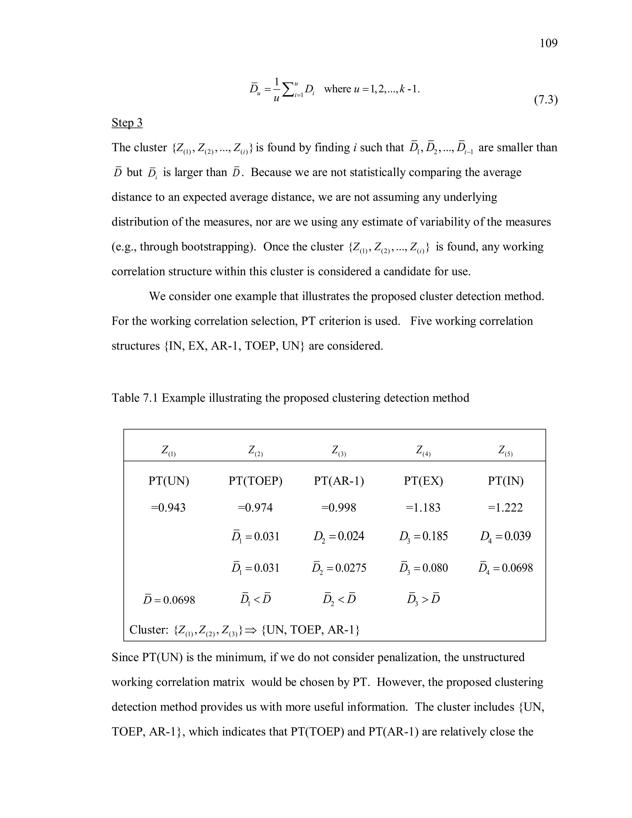
134. 107
It should be noted that both Molinari et al. (2001) and Dematteï and Molinari
(2007) used approaches based on the underlying standard uniform distribution of the
random variables. Data transformation to U(0,1) prior to the hypothesis testing is
required, in order to measure distance Di in a meaningful and comparable way. The true
distribution for a working correlation selection criterion measure in GEE depends upon
the underlying distribution of the data as well as the choice of the working correlation –
which could either be correct, over-parameterized, under-parameterized, or simply
incorrect in some other way. Thus, the set of criterion measures 1 2, ,..., kZ Z Z will not
have the same underlying distributions and individually are generally unknown. Also,
they are not independent random variables, because all of them will be functions of the
same set of n data points. However, when bias correction is used in the estimation of the
GEE robust variance estimator, it is intuitively reasonable that all iZ values associated
with either the correct or over-parameterized working correlation structures are trying to
estimate the same quantity, and would tend to “cluster” near that true value. Those
associated with ill-fitting structures should be larger, and thus skew the empirical
histogram of the set to the right. However, if all candidate models fit or over-fit the true
working correlation, all values will tend to be within the same “cluster”. It is argued that
this characterization of what is expected could be effective in identifying that cluster of
similarly fitting criterion measures from among the set of k candidates. In order to use
this approach, however, it is still necessary to scale the range of values onto a [0, 1]
range. The traditional data normalization method ( ) [ min( )]/[max( ) min( )]i if t t t t t   can
be used. However, it may be overly influenced by extreme values in this setting. For a
highly skewed distribution, it may cause those measures at the low end to appear more
similar than we would want. Additionally, the earlier work of Dematteï and Molinari
(2007) under the assumption of a uniform random sample showed that the p-value for
cluster testing would tend to be high in the small sample size setting. Practically
speaking, most analysts will not consider a large set of working correlation structures.

135. 108
To base a cluster-detection method on their hypothesis testing approach in our small
sample setting, even if their distributional assumptions were a reasonable approximation,
would allow too many working correlation structures in the cluster. The proposed
method of scaling is described in Section 7.3.
7.3 Proposed Cluster Detection Method for Working
Correlation Selection
The general idea of the work of Molinari et al. (2001) is that the mean spacing of
a cluster is lower than the overall mean spacing. A spacing smaller than the overall mean
spacing suggests that the two points are part of the same cluster. Spacing larger than the
overall mean spacing suggests that the two points are not in the same cluster. The
proposed cluster detection method is based on the idea of Molinari et al. (2001).
However, rather than using the hypothesis testing, we rely on a comparison of a spacing
to the mean spacing for a given portion to determine the cluster. This approach is
defined more precisely below.
Step 1
Let Z be any working correlation selection criterion. We consider k different working
correlation structures, including independence, which would be expected to fit poorly in
this correlated data setting. For a set of k candidate working correlation structures,
compute the working correlation selection criterion values for each candidate:
1 2, , ..., .kZ Z Z Let jZ indicate the criterion value under the j-th working correlation
structure. Then, sort jZ values from the smallest to the largest: (1) (2) ( )... kZ Z Z   .
Step 2
Obtain the spacings ( 1) ( ) , 1,2,.., 1i i iD Z Z i k    and the overall mean spacing
1
1
( 1).
k
ll
D D k


  .
Calculate the mean spacing uD for a potential cluster
(1) (2) ( 1){ , ,..., }uZ Z Z  :

136. 109
1
1
where 1,2,..., -1.
u
u ii
D D u k
u 
 
(7.3)
Step 3
The cluster (1) (2) ( ){ , ,..., }iZ Z Z is found by finding i such that 1 2 1, ,..., iD D D are smaller than
D but iD is larger than D. Because we are not statistically comparing the average
distance to an expected average distance, we are not assuming any underlying
distribution of the measures, nor are we using any estimate of variability of the measures
(e.g., through bootstrapping). Once the cluster (1) (2) ( ){ , ,..., }iZ Z Z is found, any working
correlation structure within this cluster is considered a candidate for use.
We consider one example that illustrates the proposed cluster detection method.
For the working correlation selection, PT criterion is used. Five working correlation
structures {IN, EX, AR-1, TOEP, UN} are considered.
Table 7.1 Example illustrating the proposed clustering detection method
(1)Z (2)Z (3)Z (4)Z (5)Z
PT(UN)
=0.943
PT(TOEP)
=0.974
PT(AR-1)
=0.998
PT(EX)
=1.183
PT(IN)
=1.222
1 0.031D  2 0.024D  3 0.185D  4 0.039D 
1 0.031D  2 0.0275D  3 0.080D  4 0.0698D 
0.0698D  1D D 2D D 3D D
Cluster: (1) (2) (3){ , , }Z Z Z  {UN, TOEP, AR-1}
Since PT(UN) is the minimum, if we do not consider penalization, the unstructured
working correlation matrix would be chosen by PT. However, the proposed clustering
detection method provides us with more useful information. The cluster includes {UN,
TOEP, AR-1}, which indicates that PT(TOEP) and PT(AR-1) are relatively close the

137. 110
minimum value PT(UN). Therefore, adding the structure of Toeplitz and AR-1 did not
change the estimated eigenvalues as much as when the exchangeable and independence
more restrictive assumptions were made.
7.4 Optimization function
Some researchers would prefer the most parsimonious working correlation
structure such as AR-1. Others might prefer a more flexible structure such as TOEP or
UN within the cluster, depending on the goal of the analysis, the sample size and number
of clustered measurements. An optimization function (or loss function) considering the
trade-off between bias and variability would help us to find the “best” working
correlation structure within the cluster.
Using an optimization function, the goal is to find a parsimonious structure that
closely approximates the true correlation matrix, without adding unnecessary parameters.
An appropriate optimization function should effectively penalize the working correlation
structure with many parameters when the sample size is small or the responses are
measured on many occasions. It should also be able to penalize the working correlation
structure which is parsimonious, but has a worse-fit. Therefore, the sample size (n), the
number of repeated measurements (m) and the number of parameters of the working
correlation structure (q) could be considered when constructing an optimization function.
Even though we expect the amount of penalization increases as m (number of clustered
measurements) or q (number of parameters in the correlation matrix) increase and n
decreases, a loss function must be chosen. It should be noted that the term
“optimization” is only intended to mean optimal in the sense that it minimized a
particular loss function, not a more general form of optimality.
Squared Euclidean distance is a commonly used loss function. If we consider k
cost components, the squared weighted Euclidean distance of 1 2( , ,..., )k     from the
origin is
2
1
k
j jj
w  where 1
1
k
jj
w
 . For penalizing the over-parameterized

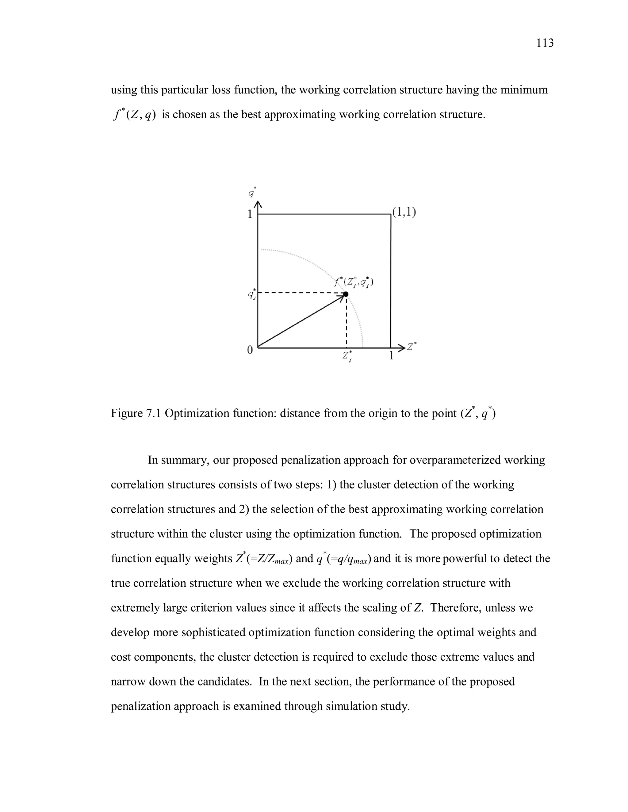
138. 111
structure, we consider two cost components: 1) the number of parameters (q) in the
working correlation structure and 2) the selection criterion measure such as PT or WR.
The q value is related to the parsimony and the selection criterion measure is related to
the goodness-of-fit of the structure to the data. Even though m and n are not considered
directly as the cost components, they are related to q and the criterion value. As m
increases, the q of the over-parameterized structure, for example, perhaps TOEPR and UNR ,
increases. As n increases, the criterion values are expected to be smaller since the model
fits the data better, and they will be closer to each other, since all correlation parameter
estimates are converging to the same quantities.
Assume the cluster includes i different working correlation structures, 1{ ,..., }iR R .
Each jR has the corresponding ( ,j jZ q ). Let max max{ | 1,..., }jZ Z j i  and
max max{ | 1,..., }jq q j i  . The weighted Euclidean distance, 2 2 1/2
[ (1 ) ]j jwZ w q  might be
considered as a loss function, depending on whether the investigator puts more
weight/emphasis on goodness of fit or on parsimony. However, we should note that the
scales of Z and q are quite different. The number q is a determined by m and the
candidate structure, R. For a given m, q is 0.5m(m-1) for UNR , and 1 for EXR and 1 for
1ARR  . On the other hand, the proposed Z is not a function of m (then number of repeated
measures on each individual) but a function of p (the number of regression parameters),
which is the dimension of the covariance matrices being compared by the generalized
eigenvalues. If ( ) ( )
ˆ ˆ
S R M IN   , PT, WR and CIC are:
1
( ) ( ) ( )
1
( ) ( ) ( )
1
( ) ( )
ˆ ˆ ˆPT [ ( ) ] / 2,
ˆ ˆ ˆWR det[ ( ) ] (0.5) ,
ˆ ˆCIC [ ] .
S R S R M IN
p
S R S R M IN
S R M IN
tr p
tr p



     
     
   
(7.4)
Since the distributions of these functions of ( )
ˆ
S R and ( )
ˆ
M IN are unknown, the range (or
variance) of each criterion measure is generally unknown. However, the simulation
results show that they are not too far away from the values in the equation (7.4) even

139. 112
when ( ) ( )
ˆ ˆ
S R M IN   . If the responses are measured at ten different time points (m=10)
and we consider two regression parameters in the marginal mean model (p=2), q ranges
from zero to 45, but PT values locate around at 1. Therefore, the normalization in (7.5) is
suggested by dividing the Z and q from each candidate model by maxZ and maxq ,
respectively.
A general expression of the optimization function for the jth
candidate model is
defined as follows:
   
2 2 1/2
max max
( , ) ,(1 )j j j j
f Z q Z Z q qw w    
(7.5)
where Zj is the selection criterion measure under the jth
candidate working correlation
structure Rj within the cluster and qj is the number of parameters of Rj. (0 1)w w  is a
common weighting factor. If w=0, the working correlation structure with the minimum
criterion value is selected as the “best” approximating working correlation structure. If
w=1, the most parsimonious structure is selected.
The proposed optimization loss function *
( , )f Z q in this dissertation weighs
both terms equally by using 0.5w  and multiplies ( , )f Z q by the constant 2 :
   
   
*
2 2 1/2
max max
2 2 1/2
max max
1/2* 2 * 2
( , ) 2 ( , )
1 1
2
2 2
.( ) ( )
f Z q f Z q
Z Z q q
Z Z q q
Z q

 
   
   
   
(7.6)
The proposed optimization function can be regarded as the Euclidean distance from the
origin in the graph of Figure 7.1 to the normalized point * *
max max( , ) ( / , / )Z q Z Z q q .
As the normalized point is further away from the origin, the corresponding the working
correlation structure has more parameters and/or a larger selection criterion measure than
other candidate models. On the other hand, the normalized point closer to the origin
indicates that the corresponding working correlation structure has a smaller selection
criterion measures and/or fewer parameters than other candidate models. Therefore,

140. 113
using this particular loss function, the working correlation structure having the minimum
*
( , )f Z q is chosen as the best approximating working correlation structure.
Figure 7.1 Optimization function: distance from the origin to the point (Z*
, q*
)
In summary, our proposed penalization approach for overparameterized working
correlation structures consists of two steps: 1) the cluster detection of the working
correlation structures and 2) the selection of the best approximating working correlation
structure within the cluster using the optimization function. The proposed optimization
function equally weights Z*
(=Z/Zmax) and q*
(=q/qmax) and it is more powerful to detect the
true correlation structure when we exclude the working correlation structure with
extremely large criterion values since it affects the scaling of Z. Therefore, unless we
develop more sophisticated optimization function considering the optimal weights and
cost components, the cluster detection is required to exclude those extreme values and
narrow down the candidates. In the next section, the performance of the proposed
penalization approach is examined through simulation study.

141. 114
7.5 Simulation Study III
The goal of the Simulation Study III is to examine the effect of the method of
penalization for the over-parameterized structure on the working correlation structure
selection presented in Sections 7.3 and 7.4. The penalization method is applied to all six
criterion measures (PT, WR, RMR, QIC, CIC, RJ).
The simulated datasets which are generated from the Simulation Study II are used
in this simulation study. We consider correlated binary responses, correlated Poisson
responses, and correlated Gaussian responses. The best approximating working
correlation structure is selected from a set of candidate structures 2Wc  {IN, EX, AR-1,
TOEP, UN}. The correct identification rates of each criterion, with and without use of
the penalization method, is used to assess performance of the criteria select the best
working correlation structure based on their minimum criterion values.
7.5.1 Simulation III Results: Correlated Binary Responses
Results of this simulation study are used to assess the performance of the
proposed method for penalizing over-parameterized working correlation structures
relative to the same measures without using it. For the correlated binary responses, the
frequencies of the working correlation structure out of 1000 independent replications are
tabulated in Table 7.2 through Table 7.13. Corresponding simulation results for cases
where the outcome vector is correlated Gaussian responses and the correlated Poisson
random variables are shown in Appendix D, Tables D.1 ~ D.12 (Gaussian) and Tables
D.13 ~ D.24 (Poisson).
7.5.1.1 The True Correlation Structure: AR-1
First, consider the simulation results for cases where the true correlation structure
C(α) is AR-1 (Table 7.2 ~ Table 7.5). Without penalization for the over-parameterized
structure, the correct identification rates (frequency/1000) of PT, WR, RMR, CIC and

142. 115
QIC are in the range of 0% to 20% and tend to decrease as n increases This is because
the estimation of the over-parameterized structure ovR as well as TR becomes more
precise as n increases. The unstructured matrix is more likely to be chosen as n increases,
reflecting the small deviations from the truth as exhibited in that particular dataset, thus
over-fitting to the data and producing a slightly smaller criterion measure. The RJ
criterion selects the correct correlation structure with approximately 30 ~ 40 % but it also
selects the exchangeable structure with approximately 30% even when n= 200.
With penalization for the over-parameterized structure, the correct identification
rates of PT, WR and CIC increase as n increases, approaching 100% by n= 200. The
RMR criterion performs worse since it uses less information of the disparity between two
covariance matrices as compared to PT, WR and CIC. The RJ criterion also performs
better as n increases, but its correct identification rates are only approximately 50% when
n= 200. Unlike other criterion measures, QIC sometimes selects the working
independence structure and its performance in working correlation selection is shown to
be lower than other criterion measures considered in this simulation study.
In small sample sizes and binary data, the correct identification rates depend
heavily on the strength of the correlation coefficients of TR and the size of the matrix
(m). When the true correlations are low, and the size of the matrix small (Table 7.2), the
unstructured matrix is still preferred by PT, WR, RMR and CIC in the unpenalized
setting at similar rates with AR-1, which is the true correlation structure in this case.
Penalization improves the correct identification dramatically. If the number of repeated
measurements is large and the true correlation coefficient is low (Table 7.4), the proposed
penalization method cannot effectively penalize the unstructured matrix. Even though
the bias-corrected sandwich variance estimator is used, the sandwich variance estimator
under the unstructured matrix is still severely negatively biased in small samples. Thus,
the proposed clustering detection method tends to capture the unstructured matrix only.

143. 116
If the true α parameter is high (Tables 7.3 and 7.5), the true underlying correlation
structure is more distinguishable from other structures. In this case, the disparity between
the variance estimate under TR and the variance estimate under the misspecified structure
becomes large. Moreover, the negative bias of the sandwich variance estimator under the
over-parameterized structure is reduced for the high true α parameter. Therefore, TR is
more likely to be included in the cluster by the proposed cluster detection method. Even
if the criterion measure under the over-parameterized structure, especially UNR , is the
minimum, the optimization function selects the parsimonious TR by penalizing the over-
parameterized structures.
Although the percent correct selection using penalization is similar among PT,
WR, and CIC, both PT and WR tend to outperform CIC in most cases. The measure
based only on the largest generalized eigenvalue (RMR) generally performs better than
the others when the true underlying structure is more complicated (TOEP and UN), and
worse for the simple structures. The RJ criterion is clearly inferior to the others.
We note that a variation of this method could be used without first identifying a cluster,
but rather moving directly to the use of the optimization function using all candidate
structures. This would be useful in settings where the correlations are all expected to be
quite low and/or when all candidate structures would be expected to fit reasonably well.

144. 117
Table 7.2 Frequencies of the working correlation structure identified using PT,
WR,RMR, CIC, QIC and RJ with/without considering penalization for the
over-parameterized structures from 1000 independent replications
(Correlated binary response; C(α): AR-1(0.3), m=4).
n Criterion
Without penalization With penalization
IN EX AR-1 TOEP UN IN EX AR-1 TOEP UN
20
PT 0 15 117 457 411 15 83 346 88 468
WR 0 17 123 463 397 14 85 349 95 457
RMR 0 17 128 400 455 87 36 219 75 583
CIC 10 68 194 318 410 16 77 346 87 474
QIC 10 68 194 318 410 316 79 197 125 283
RJ 0 306 338 209 147 29 406 560 1 4
30
PT 0 0 100 475 425 2 70 410 55 463
WR 0 1 114 474 411 2 70 422 61 445
RMR 0 0 102 421 477 70 36 270 62 562
CIC 0 41 204 350 405 4 79 412 53 452
QIC 0 41 204 350 405 326 85 221 92 276
RJ 0 374 353 177 96 5 440 555 0 0
50
PT 0 0 93 490 417 0 69 569 16 346
WR 0 1 102 484 413 0 74 578 17 331
RMR 0 0 81 429 490 68 35 376 26 495
CIC 0 28 181 369 422 0 65 563 16 356
QIC 0 28 181 369 422 364 91 239 76 230
RJ 0 330 386 192 92 1 454 545 0 0
100
PT 0 0 83 481 436 0 39 825 2 134
WR 0 0 87 497 416 0 40 831 2 127
RMR 0 0 65 391 544 30 35 563 14 358
CIC 0 7 199 368 426 0 39 800 3 158
QIC 0 7 199 368 426 422 122 249 37 170
RJ 0 342 382 197 79 0 475 525 0 0
200
PT 0 0 83 455 462 0 9 973 0 18
WR 0 0 96 460 444 0 10 973 0 17
RMR 0 0 65 365 570 12 15 771 8 194
CIC 0 1 218 328 453 0 14 961 0 25
QIC 0 1 218 328 453 401 138 307 12 142
RJ 0 357 375 188 80 0 471 529 0 0

145. 118
Table 7.3 Frequencies of the working correlation structure identified using PT,
WR,RMR, CIC, QIC and RJ with/without considering penalization for the
over-parameterized structures from 1000 independent replications
(Correlated binary response; C(α): AR-1(0.6), m=4).
n Criterion
Without penalization With penalization
IN EX AR-1 TOEP UN IN EX AR-1 TOEP UN
20
PT 35 55 197 209 504 36 111 685 10 158
WR 35 56 200 203 506 35 110 686 26 143
RMR 15 24 83 150 728 68 72 426 33 401
CIC 42 96 210 224 428 39 121 679 14 147
QIC 240 169 139 204 248 338 169 259 85 149
RJ 35 278 348 129 210 37 441 521 0 1
30
PT 2 27 90 149 732 13 62 807 3 115
WR 2 28 92 148 730 13 58 813 8 108
RMR 7 11 62 131 789 45 51 563 17 324
CIC 2 59 132 226 581 14 82 799 1 104
QIC 264 196 109 158 273 376 172 253 64 135
RJ 2 309 357 112 220 14 431 555 0 0
50
PT 5 11 73 118 793 5 27 932 0 36
WR 5 11 76 120 788 5 25 940 0 30
RMR 7 10 68 136 779 23 55 739 10 173
CIC 5 25 141 219 610 5 49 912 0 34
QIC 244 194 114 167 281 379 166 297 42 116
RJ 5 306 358 113 218 5 474 521 0 0
100
PT 0 3 28 78 891 0 5 992 0 3
WR 0 3 25 74 898 0 5 993 0 2
RMR 1 1 75 139 784 2 18 925 4 51
CIC 0 6 133 164 697 0 8 990 0 2
QIC 283 225 99 130 263 413 191 283 12 101
RJ 0 340 338 125 197 0 478 522 0 0
200
PT 0 0 26 62 912 0 0 1000 0 0
WR 0 0 19 65 916 0 0 1000 0 0
RMR 0 0 71 129 800 0 5 991 0 4
CIC 0 0 108 193 699 0 0 1000 0 0
QIC 287 228 130 117 238 422 198 315 6 59
RJ 0 308 393 116 183 0 448 552 0 0

146. 119
Table 7.4 Frequencies of the working correlation structure identified using PT,
WR,RMR, CIC, QIC and RJ with/without considering penalization for the
over-parameterized structures from 1000 independent replications
(Correlated binary response; C(α): AR-1(0.3), m=6).
n Criterion
Without penalization With penalization
IN EX AR-1 TOEP UN IN EX AR-1 TOEP UN
20
PT 1 5 64 215 715 2 16 196 123 663
WR 0 5 64 215 716 2 16 193 137 652
RMR 4 8 14 38 936 29 6 59 37 869
CIC 19 24 71 204 682 2 18 193 125 662
QIC 150 101 134 249 366 307 48 157 184 304
RJ 3 199 416 177 205 18 414 560 7 1
30
PT 0 1 19 77 903 0 6 170 41 783
WR 0 1 20 76 903 0 7 175 52 766
RMR 8 7 8 20 957 22 5 66 27 880
CIC 11 12 44 109 824 0 5 154 54 787
QIC 143 118 105 169 465 321 56 140 97 386
RJ 0 202 385 158 255 2 438 559 1 0
50
PT 0 0 5 9 986 0 5 253 13 729
WR 0 0 5 11 984 0 7 287 19 687
RMR 4 4 3 6 983 7 11 105 14 863
CIC 4 13 28 58 897 0 5 224 18 753
QIC 193 108 116 135 448 355 63 182 59 341
RJ 0 249 367 141 243 0 450 550 0 0
100
PT 0 0 0 2 998 0 2 584 4 410
WR 0 0 0 2 998 0 1 632 2 365
RMR 0 0 5 4 991 3 6 252 8 731
CIC 0 7 32 47 914 0 2 558 4 436
QIC 211 147 120 127 395 366 87 200 38 309
RJ 0 265 384 137 214 0 447 553 0 0
200
PT 0 0 0 3 997 0 0 923 0 77
WR 0 0 0 3 997 0 0 944 0 56
RMR 0 0 2 3 995 1 1 455 4 539
CIC 1 0 29 80 890 0 1 887 0 112
QIC 243 176 120 123 338 410 105 250 21 214
RJ 0 301 391 155 153 0 468 532 0 0

147. 120
Table 7.5 Frequencies of the working correlation structure identified using PT,
WR,RMR, CIC, QIC and RJ with/without considering penalization for the
over-parameterized structures from 1000 independent replications
(Correlated binary response; C(α): AR-1(0.6), m=6).
n Criterion
Without penalization With penalization
IN EX AR-1 TOEP UN IN EX AR-1 TOEP UN
20
PT 5 31 134 334 496 5 40 607 31 317
WR 5 31 148 320 496 5 38 615 58 284
RMR 2 9 51 102 836 20 14 243 42 681
CIC 12 50 155 325 458 6 47 587 59 301
QIC 226 160 135 243 236 341 129 263 106 161
RJ 5 294 376 176 149 6 445 546 3 0
30
PT 1 19 81 242 657 1 23 728 7 241
WR 1 19 91 227 662 1 22 705 71 201
RMR 5 3 34 95 863 21 15 361 24 579
CIC 2 32 132 249 585 1 34 665 56 244
QIC 204 183 143 190 280 338 131 273 67 191
RJ 1 304 361 154 180 1 464 530 5 0
50
PT 0 2 37 130 831 0 4 917 0 79
WR 0 2 39 127 832 0 2 918 23 57
RMR 1 1 27 65 906 3 10 581 9 397
CIC 0 7 75 165 753 0 6 873 13 108
QIC 205 171 131 183 310 317 140 290 47 206
RJ 0 321 349 148 182 0 467 532 1 0
100
PT 0 0 7 26 967 0 0 999 0 1
WR 0 0 6 25 969 0 0 999 0 1
RMR 0 0 18 53 929 0 1 873 3 123
CIC 0 0 38 107 855 0 0 992 1 7
QIC 250 157 128 118 347 342 135 331 19 173
RJ 0 301 345 141 213 0 499 501 0 0
200
PT 0 0 5 11 984 0 0 1000 0 0
WR 0 0 5 14 981 0 0 1000 0 0
RMR 0 0 14 38 948 0 0 991 0 9
CIC 0 0 47 77 876 0 0 1000 0 0
QIC 258 231 113 111 287 363 199 312 10 116
RJ 0 329 353 137 181 0 472 528 0 0

148. 121
7.5.1.2 The True Correlation Structure: Exchangeable
When the true correlation structure is exchangeable, similar patterns are identified
except the RJ criterion. As discussed above, the RJ criterion is known to have a tendency
to select the exchangeable structure regardless of the true correlation structure. If the true
correlation structure is exchangeable, its performance is better than PT, WR and CIC.
However, the true underlying correlation structure is generally unknown.
The improvement in correct identification seen when the true structure is
exchangeable and the correlation is high is not as strong as that seen when it is an AR-1
structure with high correlation, unless the sample size is 200.

149. 122
Table 7.6 Frequencies of the working correlation structure identified using PT,
WR,RMR, CIC, QIC and RJ with/without considering penalization for the
over-parameterized structures from 1000 independent replications
(Correlated binary response; C(α): EX(0.3), m=4).
n Criterion
Without penalization With penalization
IN EX AR-1 TOEP UN IN EX AR-1 TOEP UN
20
PT 22 69 31 169 709 37 326 141 78 418
WR 22 75 31 164 708 29 332 141 89 409
RMR 44 55 30 77 794 184 130 81 35 570
CIC 58 106 83 173 580 47 316 140 70 427
QIC 189 89 173 156 393 323 111 197 80 289
RJ 30 313 60 258 339 33 868 88 4 7
30
PT 2 55 9 113 821 11 450 110 42 387
WR 2 51 10 116 821 7 466 115 45 367
RMR 54 54 26 76 790 247 146 76 29 502
CIC 33 105 63 144 655 18 439 109 34 400
QIC 180 83 225 114 398 322 105 240 49 284
RJ 4 339 29 253 375 5 950 43 0 2
50
PT 0 16 1 94 889 1 640 87 10 262
WR 0 16 1 96 887 0 652 92 10 246
RMR 36 43 17 69 835 293 181 67 17 442
CIC 13 106 40 142 699 3 604 85 10 298
QIC 218 72 255 96 359 370 109 272 35 214
RJ 0 337 7 259 397 0 985 15 0 0
100
PT 0 11 0 71 918 0 887 29 1 83
WR 0 10 0 71 919 0 895 31 2 72
RMR 28 47 4 66 855 499 184 44 7 266
CIC 2 106 11 150 731 0 863 30 0 107
QIC 243 66 309 79 303 397 108 315 10 170
RJ 0 331 0 278 391 0 1000 0 0 0
200
PT 0 13 0 68 919 0 990 3 0 7
WR 0 13 0 70 917 0 992 3 0 5
RMR 6 53 0 65 876 655 219 14 2 110
CIC 0 112 2 168 718 0 986 1 0 13
QIC 252 59 358 68 263 440 121 345 5 89
RJ 0 364 0 260 376 0 1000 0 0 0

150. 123
Table 7.7 Frequencies of the working correlation structure identified using PT,
WR,RMR, CIC, QIC and RJ with/without considering penalization for the
over-parameterized structures from 1000 independent replications
(Correlated binary response; C(α): EX(0.6), m=4).
n Criterion
Without penalization With penalization
IN EX AR-1 TOEP UN IN EX AR-1 TOEP UN
20
PT 100 161 28 251 460 100 495 264 24 117
WR 100 157 28 252 463 100 477 273 46 104
RMR 38 92 20 151 699 168 328 75 31 398
CIC 114 214 69 239 364 116 489 248 29 118
QIC 311 162 162 166 199 388 208 268 49 87
RJ 100 403 47 244 206 102 783 115 0 0
30
PT 72 122 14 172 620 72 608 219 8 93
WR 72 120 14 172 622 72 600 226 25 77
RMR 26 92 15 125 742 172 469 62 10 287
CIC 76 190 57 197 480 76 619 198 11 96
QIC 299 147 189 133 232 393 185 276 47 99
RJ 72 394 14 225 295 72 846 81 1 0
50
PT 25 64 3 136 772 25 767 177 2 29
WR 25 64 3 130 778 25 754 181 14 26
RMR 18 84 3 121 774 221 580 42 3 154
CIC 26 158 33 221 562 25 773 166 4 32
QIC 277 122 242 101 258 395 173 304 28 100
RJ 25 375 1 261 338 25 915 60 0 0
100
PT 2 28 0 83 887 2 912 82 0 4
WR 2 25 0 77 896 2 912 82 1 3
RMR 4 86 0 133 777 207 750 7 0 36
CIC 2 142 10 185 661 2 919 75 0 4
QIC 305 88 300 76 231 462 120 335 9 74
RJ 2 376 0 234 388 2 962 36 0 0
200
PT 0 8 0 63 929 0 975 25 0 0
WR 0 5 0 55 940 0 974 26 0 0
RMR 0 77 0 116 807 224 774 2 0 0
CIC 0 131 1 181 687 0 980 20 0 0
QIC 336 50 369 64 181 449 107 391 3 50
RJ 0 365 0 253 382 0 986 14 0 0

151. 124
Table 7.8 Frequencies of the working correlation structure identified using PT,
WR,RMR, CIC, QIC and RJ with/without considering penalization for the
over-parameterized structures from 1000 independent replications
(Correlated binary response; C(α): EX(0.3), m=6).
n Criterion
Without penalization With penalization
IN EX AR-1 TOEP UN IN EX AR-1 TOEP UN
20
PT 5 58 4 203 730 7 229 70 88 606
WR 4 64 6 199 727 6 216 71 113 594
RMR 22 26 15 45 892 50 96 22 29 803
CIC 33 76 32 194 665 16 214 67 99 604
QIC 158 91 161 164 426 275 105 185 98 337
RJ 6 402 12 283 297 7 950 38 3 2
30
PT 1 19 0 100 880 2 235 47 41 675
WR 1 20 0 99 880 2 223 46 87 642
RMR 14 22 6 42 916 53 123 18 18 788
CIC 8 51 26 117 798 3 216 43 50 688
QIC 158 59 165 126 492 268 85 200 58 389
RJ 1 350 2 280 367 1 980 17 1 1
50
PT 0 2 0 21 977 0 425 14 8 553
WR 0 1 0 22 977 0 459 15 25 501
RMR 5 14 4 19 958 41 218 22 13 706
CIC 5 37 7 72 879 0 373 16 15 596
QIC 159 63 242 73 463 288 100 246 35 331
RJ 0 340 1 259 400 0 998 2 0 0
100
PT 0 3 0 9 988 0 827 3 0 170
WR 0 3 0 11 986 0 866 3 1 130
RMR 1 14 1 19 965 21 439 13 6 521
CIC 0 41 2 69 888 0 728 2 0 270
QIC 222 60 263 77 378 336 105 282 17 260
RJ 0 316 0 256 428 0 1000 0 0 0
200
PT 0 0 0 5 995 0 989 0 0 11
WR 0 0 0 5 995 0 992 0 0 8
RMR 0 6 0 14 980 15 764 4 2 215
CIC 0 49 0 73 878 0 965 0 0 35
QIC 279 61 298 70 292 430 126 293 7 144
RJ 0 315 0 278 407 0 1000 0 0 0

152. 125
Table 7.9 Frequencies of the working correlation structure identified using PT,
WR,RMR, CIC, QIC and RJ with/without considering penalization for the
over-parameterized structures from 1000 independent replications
(Correlated binary response; C(α): EX(0.6), m=6).
n Criterion
Without penalization With penalization
IN EX AR-1 TOEP UN IN EX AR-1 TOEP UN
20
PT 50 162 12 287 489 53 355 256 100 236
WR 50 164 12 284 490 53 350 267 107 223
RMR 14 64 14 118 790 63 263 25 24 625
CIC 72 214 44 233 437 63 384 225 112 216
QIC 275 171 133 188 233 361 193 252 80 114
RJ 50 470 7 266 207 51 842 99 8 0
30
PT 22 127 2 272 577 22 434 313 38 193
WR 22 125 1 273 579 22 396 312 103 167
RMR 8 51 5 86 850 40 409 16 10 525
CIC 25 189 21 262 503 25 451 277 62 185
QIC 284 183 112 174 247 371 215 250 58 106
RJ 22 453 0 277 248 22 855 123 0 0
50
PT 7 47 0 122 824 7 586 307 8 92
WR 7 47 0 118 828 7 571 311 54 57
RMR 3 31 0 61 905 18 740 2 4 236
CIC 9 112 12 167 700 8 606 278 30 78
QIC 254 135 178 140 293 349 180 289 66 116
RJ 7 377 0 257 359 7 872 121 0 0
100
PT 0 6 0 24 970 0 797 202 0 1
WR 0 6 0 24 970 0 789 203 8 0
RMR 0 36 0 58 906 6 977 0 0 17
CIC 0 90 1 135 774 0 815 179 1 5
QIC 287 82 253 94 284 371 156 333 47 93
RJ 0 379 0 235 386 0 922 78 0 0
200
PT 0 3 0 8 989 0 913 87 0 0
WR 0 3 0 4 993 0 912 88 0 0
RMR 0 29 0 56 915 0 1000 0 0 0
CIC 0 75 0 143 782 0 915 85 0 0
QIC 317 55 338 57 233 410 128 383 24 55
RJ 0 354 0 255 391 0 967 33 0 0

153. 126
7.5.1.3 The True Correlation Structure: Toeplitz
When the true correlation structure is Toeplitz (defined in Table 3.2) and the
distribution is a multivariate binomial, PT, WR and CIC perform better by penalizing
over-parameterized structures (Table 7.10 and Table 7.11). Note that both TOEPR and
UNR are penalized. Since UNR contains more parameters, the optimization function
penalizes UNR more than TOEPR . In this simulation setting, the true 44 Toeplitz
correlation structure has considerable similarity to the exchangeable structure, with most
of its correlations being exactly .25. Therefore, EXR is chosen at similar rates as TOEPR ,
which is the true correlation structure. Whereas PT and WR with penalization perform
better as n increases, the accuracy rates of CIC with penalization decrease for 44 matrix
since EXR is more likely to be chosen by CIC as n increases (Table 7.10). For the 6 6
Toeplitz structure, we do not observe this decrease in correct identification as n gets
larger in CIC, since the underlying Toeplitz matrix now is more easily distinguished from
exchangeable (Table 7.11).
The RMR and QIC do not perform well as much as PT, WR and CIC when the
proposed penalization method is used. The RJ criterion still tends to select the
exchangeable structure. Furthermore, since the true underlying Toeplitz structure
(defined in is Table 3.2) has similarity to the exchangeable structure, it selects the
exchangeable structure with 100% when n = 100 and 200.

154. 127
Table 7.10 Frequencies of the working correlation structure identified using PT,
WR,RMR, CIC, QIC and RJ with/without considering penalization for the
over-parameterized structures from 1000 independent replications
(Correlated binary response; C(α): TOEP, m=4).
n
Criter
ion
Without penalization With penalization
IN EX AR-1 TOEP UN IN EX AR-1 TOEP UN
20
PT 15 277 11 132 565 24 428 42 310 196
WR 13 278 11 133 565 21 419 44 342 174
RMR 26 50 6 116 802 232 155 5 192 416
CIC 59 266 27 153 495 67 417 37 275 204
QIC 196 167 191 144 302 354 152 162 144 188
RJ 15 524 5 211 245 20 950 19 9 2
30
PT 3 233 1 117 646 8 464 23 382 123
WR 3 233 1 122 641 7 420 23 443 107
RMR 17 33 0 105 845 343 109 0 213 335
CIC 22 249 9 167 553 42 465 21 338 134
QIC 178 170 231 146 275 370 165 186 131 148
RJ 3 538 2 217 240 5 982 12 1 0
50
PT 1 143 0 64 792 2 473 7 475 43
WR 1 143 0 64 792 1 401 7 563 28
RMR 6 19 0 86 889 562 87 0 190 161
CIC 7 171 1 170 651 22 540 6 377 55
QIC 167 130 260 147 296 359 139 212 152 138
RJ 1 492 1 219 287 1 997 2 0 0
100
PT 0 61 0 65 874 0 432 0 565 3
WR 0 61 0 66 873 0 336 0 662 2
RMR 2 3 0 77 918 850 11 0 107 32
CIC 0 74 0 176 750 6 623 0 367 4
QIC 191 80 297 155 277 384 103 244 160 109
RJ 0 465 0 257 278 0 1000 0 0 0
200
PT 0 9 0 62 929 0 405 0 595 0
WR 0 9 0 62 929 0 249 0 751 0
RMR 0 0 0 80 920 950 1 0 49 0
CIC 0 9 0 217 774 1 725 0 274 0
QIC 161 54 321 173 291 367 108 270 175 80
RJ 0 463 0 256 281 0 1000 0 0 0

155. 128
Table 7.11 Frequencies of the working correlation structure identified using PT,
WR,RMR, CIC, QIC and RJ with/without considering penalization for the
over-parameterized structures from 1000 independent replications
(Correlated binary response; C(α): TOEP, m=6).
n
Criter
ion
Without penalization With penalization
IN EX AR-1 TOEP UN IN EX AR-1 TOEP UN
20
PT 3 153 1 382 461 13 207 76 426 278
WR 3 152 1 384 460 10 193 82 464 251
RMR 3 29 6 125 837 67 102 8 105 718
CIC 29 175 14 369 413 25 227 75 385 288
QIC 202 158 159 230 251 327 147 170 180 176
RJ 3 546 1 267 183 8 942 35 13 2
30
PT 2 106 0 327 565 6 168 52 553 221
WR 2 106 0 323 569 4 137 57 627 175
RMR 7 15 5 118 855 63 162 8 116 651
CIC 8 125 3 345 519 17 215 47 461 260
QIC 187 139 170 237 267 313 136 192 181 178
RJ 2 523 0 265 210 4 968 15 13 0
50
PT 0 44 0 250 706 0 87 29 770 114
WR 0 44 0 253 703 0 53 29 839 79
RMR 1 9 1 78 911 28 268 4 154 546
CIC 1 55 0 303 641 4 137 29 670 160
QIC 207 94 213 213 273 340 117 221 157 165
RJ 0 473 0 281 246 1 987 11 1 0
100
PT 0 2 0 97 901 0 23 8 962 7
WR 0 2 0 99 899 0 2 8 984 6
RMR 0 6 0 50 944 19 513 0 210 258
CIC 0 2 0 178 820 0 42 8 939 11
QIC 203 74 259 151 313 348 88 267 139 158
RJ 0 440 0 266 294 0 997 3 0 0
200
PT 0 0 0 37 963 0 3 0 997 0
WR 0 0 0 40 960 0 0 0 1000 0
RMR 0 0 0 33 967 8 800 0 157 35
CIC 0 0 0 179 821 0 9 0 991 0
QIC 238 66 264 127 305 372 87 282 118 141
RJ 0 456 0 249 295 0 1000 0 0 0

156. 129
7.5.1.4 The True Correlation Structure: Unstructured
Lastly, if the true correlation structure is unstructured (defined in Table 3.2), the
proposed penalization method in the binary data setting decreases the correct
identification rates of the criterion measures when the matrix size is small 4  4 ( Table
7.12). The 4  4 true underlying structure in this simulation study has considerable
similarity with AR-1. Therefore, AR-1 is more likely to be chosen in small samples since
both TOEPR and UNR are penalized. However, when m= 6, all criterion measures, whether
penalized or not, perform effectively the same in the binary data setting when the
underlying structure is unstructured.
7.5.2 Simulation Results III: Correlated Gaussian
Responses and Poisson Responses
The frequencies of the working correlation structure out of 1000 independent
replications for the correlated Gaussian responses (Table D.1 ~ Table D.12) and for the
correlated Poisson responses (Table D.13 ~ Table D.24) are presented in Appendix D.
They present similar results to the simulation results for the correlated binary responses.

157. 130
Table 7.12 Frequencies of the working correlation structure identified using PT,
WR,RMR, CIC, QIC and RJ with/without considering penalization for the
over-parameterized structures from 1000 independent replications
(Correlated binary response; C(α): UN, m=4).
n Criterion
Without penalization With penalization
IN EX AR-1 TOEP UN IN EX AR-1 TOEP UN
20
PT 38 62 253 245 402 1 76 515 7 401
WR 38 65 255 238 404 0 82 529 13 376
RMR 5 8 75 104 808 11 96 510 22 361
CIC 47 87 229 265 372 0 96 575 11 318
QIC 260 196 135 238 171 115 124 413 23 325
RJ 38 308 317 126 211 1 505 418 0 76
30
PT 7 30 195 225 543 0 34 503 3 460
WR 7 30 211 209 543 0 37 537 4 422
RMR 2 5 38 76 879 3 43 511 8 435
CIC 10 49 200 253 488 0 44 606 5 345
QIC 241 170 130 247 212 80 76 495 9 340
RJ 7 283 366 117 227 2 498 442 0 58
50
PT 4 8 175 176 637 0 12 454 1 533
WR 4 8 186 165 637 0 12 511 1 476
RMR 0 1 24 39 936 0 15 506 0 479
CIC 4 15 174 214 593 0 17 626 0 357
QIC 249 192 133 226 200 41 45 545 1 368
RJ 4 300 309 131 256 0 494 480 0 26
100
PT 0 1 107 104 788 0 0 371 0 629
WR 0 1 113 98 788 0 0 451 0 549
RMR 0 0 5 9 986 0 0 416 0 584
CIC 0 3 95 129 773 0 1 627 0 372
QIC 234 195 99 228 244 13 8 575 0 404
RJ 0 282 305 75 338 0 542 454 0 4
200
PT 0 0 39 32 929 0 0 199 0 801
WR 0 0 43 28 929 0 0 310 0 690
RMR 0 0 0 0 1000 0 0 260 0 740
CIC 0 0 27 45 928 0 0 549 0 451
QIC 249 190 92 189 280 1 2 594 0 403
RJ 0 303 256 90 351 0 543 457 0 0

158. 131
Table 7.13 Frequencies of the working correlation structure identified using PT,
WR,RMR, CIC, QIC and RJ with/without considering penalization for the
over-parameterized structures from 1000 independent replications
(Correlated binary response; C(α): UN, m=6).
n Criterion
Without penalization With penalization
IN EX AR-1 TOEP UN IN EX AR-1 TOEP UN
20
PT 5 39 68 467 421 0 103 340 55 502
WR 5 35 79 459 422 0 79 318 121 482
RMR 10 21 17 74 878 10 174 290 44 482
CIC 25 102 108 355 410 0 125 312 106 457
QIC 215 142 214 210 219 176 105 244 33 442
RJ 5 396 147 272 180 0 716 187 11 86
30
PT 2 10 48 417 523 0 58 323 28 591
WR 2 9 59 407 523 0 41 291 89 579
RMR 3 16 5 61 915 3 116 295 27 559
CIC 12 58 84 334 512 0 63 324 96 517
QIC 212 149 220 207 212 140 94 250 32 484
RJ 2 385 91 274 248 0 828 109 6 57
50
PT 0 1 14 338 647 0 29 243 8 720
WR 0 1 16 336 647 0 15 231 55 699
RMR 1 7 2 13 977 1 69 237 3 690
CIC 1 34 45 279 641 0 42 282 49 627
QIC 237 149 215 133 266 89 80 239 7 585
RJ 0 386 46 267 301 0 903 66 0 31
100
PT 0 0 5 174 821 0 7 145 0 848
WR 0 0 6 173 821 0 1 143 19 837
RMR 0 1 0 3 996 0 39 140 0 821
CIC 0 6 16 163 815 0 16 174 22 788
QIC 241 138 264 67 290 44 43 187 1 725
RJ 0 370 9 241 380 0 969 9 0 22
200
PT 0 0 0 66 934 0 0 70 0 930
WR 0 0 1 65 934 0 0 72 3 925
RMR 0 0 0 0 1000 0 8 78 0 914
CIC 0 1 0 65 934 0 1 102 5 892
QIC 213 130 250 53 354 17 9 153 1 820
RJ 0 380 1 181 438 0 995 2 0 3

159. 132
CHAPTER 8
ANOTHER PENALIZATION APPROACH USING BOOSTRAPPED
DATA
The motivation behind the proposed penalization approach using the cluster
detection is that the over-parameterized structure and the true correlation structure have
similar measures, but the misspecified structure does not. To find the group (or cluster)
of working correlation structures that are similar to each other, the cluster detection
method based on the spacings of the order statistics of the criterion measures was
proposed in chapter 7. In this chapter, we discuss another method we investigated to find
the group of working correlation structures which are not statistically different.
8.1 Incorporating Measure Variability into the Selection
An over-parameterized model and the true model would tend to have similar
measures, but in practice, there is no reliable rule to determine how small a deviation
between the two measures implies “similar.” The bootstrap method can be used to
construct an estimate of the standard deviation of the proposed selection measures. This
information can be incorporated into the covariance structure selection process by using it
to determine if two measures are statistically different from each other. The approach
proposed is to fit the data using different working correlation structures, compute the
selection criterion for each, find the bootstrap variance of that measure, and incorporate
the information into a classical ANOVA analysis and follow-up comparisons to look for
measures that differ significantly. This approach results in identification of groups of
working correlation models with criterion measures that are “not” statistically different
from each other. Then, we would propose to declare the most parsimonious structure
within the (best) group as the best approximating structure.

160. 133
8.2 Simulation Study IV
The effectiveness of this approach in the GEE covariance selection problem is
assessed in the simulation study IV. Figure 8.1 shows a flow chart of a specific
simulation process. The empirical bootstrap method will be used, in which B bootstrap
samples from the observed (simulated) data are drawn using resampling with
replacement. For this simulation experiment, B is defined as the half of the sample size
(i.e., B = 0.5n). To get one bootstrap sample, a simple random sample of size n is taken,
with replacement, from the n independent vectors of the observed data. This process is
repeated until B bootstrap samples are generated by resampling with replacement and
they are treated as a set of B independent real samples from population.
For each bootstrap sample, five GEE models under different working correlation
structures (IN, EX, AR-1, TOEP, UN) are fit. Mean models are correctly specified so
that effects of different working correlation assumptions are the only model fit
component being assessed. For each GEE model fit, the PT, WR, RMR, CIC and RJ are
calculated. That is, within one bootstrap sample, PT(IN), PT(EX), PT(AR-1),
PT(TOEP), PT(UN) are obtained. This is repeated until we have obtained B samples of
each PT(IN), PT(EX), PT(AR-1), PT(TOEP), and PT(UN) measure. Then, an applicable
hypothesis testing procedure, such as ANOVA is performed to compare the mean of the
B criterion measures under each of the five different working structures. Since small
values of the selection criterion measures indicate strong fit to the data, the goal is to find
the set of candidate working covariance models whose criterion measures are not
significantly different from the minimum value for that criterion. Once those groups are
found (e.g., through Tukey’s HSD testing) the most parsimonious working correlation is
chosen as the best working correlation structure. If two or more structures in that group
have the same number of parameters (e.g., AR-1 and EX), we propose the working
correlation structure with the lowest criterion value will be chosen as “best”. We assess

161. 134
the performance of the bootstrapping approach by 100 independent replicated
simulations.
In the Simulation Study IV, we consider the correlated binary responses. The
simulation design is a factorial with the factor levels described in Table 8.1. We denote
PT, WR, RMR, CIC, QIC and RJ applying the penalization method using bootstrapped
data by PTb, WRb, RMRb, CICb , QICb and RJb.

162. 135
Figure 8.1 Flow chart of the bootstrap simulation study
Example Simulation: True correlation: AR-1, α=0.4
cluster size m=4; sample size n=100

Generate one simulation dataset 1
1 1
2 2
1
n n
Y X
Y X
Y X
 
 
 
 
 
 
where 1 2( , , )i i i imY Y Y Y 

Using bootstrapping, randomly extract B datasets
2 3, , B

For each dataset 1 2 3, , , B , run five models with different working
correlation assumptions (IN, EX, AR-1, TOEP,UN) and calculate PT, WR, CIC,
RMR, QIC, RJ criterion values

Bootstrapped
data
Group
(IN)
Group
(EX)
Group
(AR-1)
Group
(TOEP)
Group
(UN)
1 PT(IN)1 PT(EX)1 PT(AR-1)1 PT(TOEP)1 PT(UN)1
2 PT(IN)2 PT(EX)2 PT(AR-1)2 PT(TOEP)2 PT(UN)2
B PT(IN)B PT(EX)B PT(AR-1)B PT(TOEP)B PT(UN)B

Run ANOVA and Tukey’s grouping

Extract the working correlation structures in the Tukey’s group containing the
minimum group mean. The most parsimonious structure within the group is
selected as the best working correlation structure.

The number of independent simulations = 100?
No
 Yes
END

163. 136
Table 8.1 Simulation Study IV Design Parameters
Factor Levels
Distribution (D) Correlated binary responses
1 1 2 2logit( ) ,it t tx x    where 1tx and 2tx are
independently generated from the uniform
distribution U[0.5, 1]. and 1 2 0.3  
Response vector dimension (m) m = 4, 6
True Correlation Structure
C(α)
Exchangeable: EX( ), 0.3,0.7  
Autoregressive of order 1: AR-1( ), 0.3,0.7  
Working Correlation structure
R(α)
Independence (IN), Exchangeable (EX),
Autoregressive (AR-1), Toeplitz (TOEP), and
unstructured (UN).
Sample Sizes (n) n = 100, 200
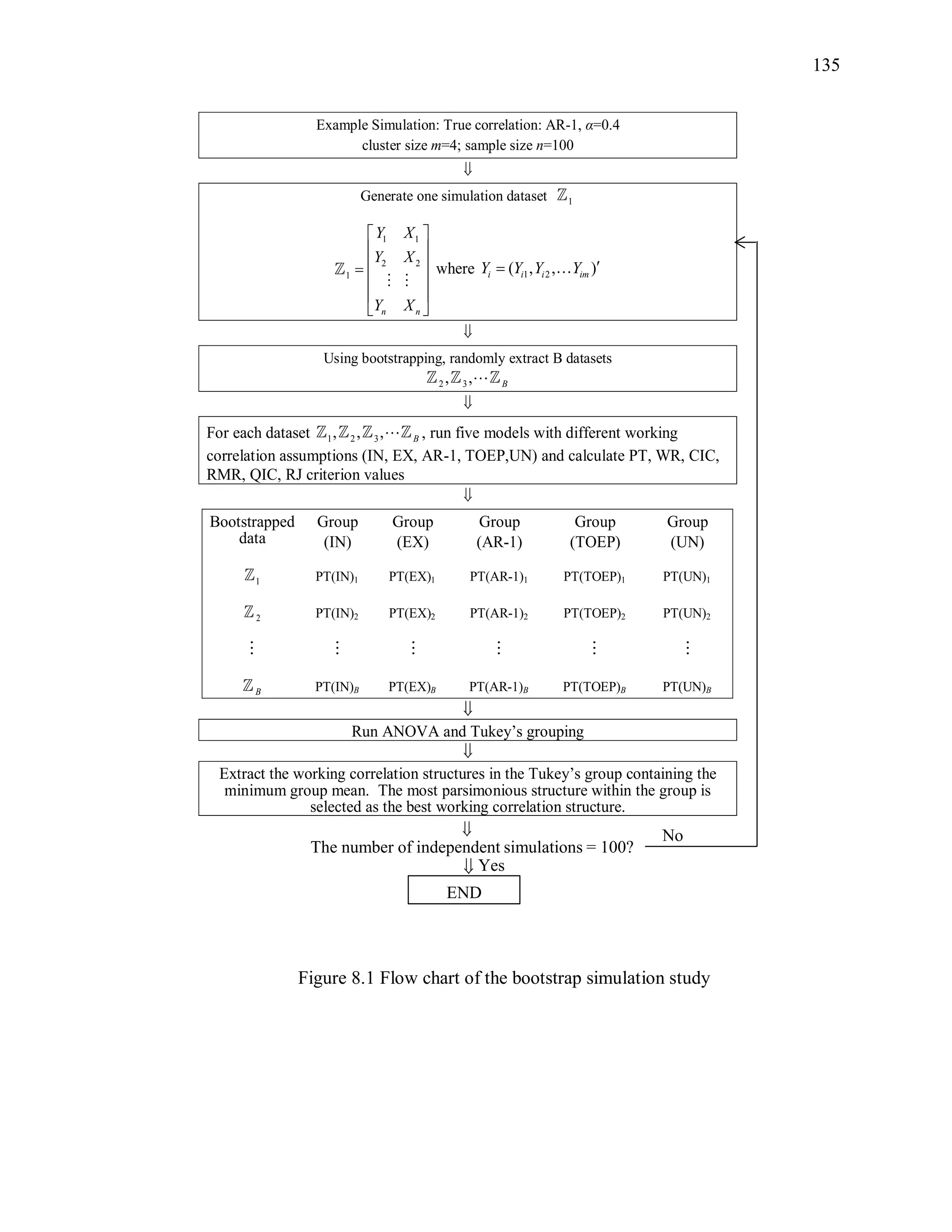
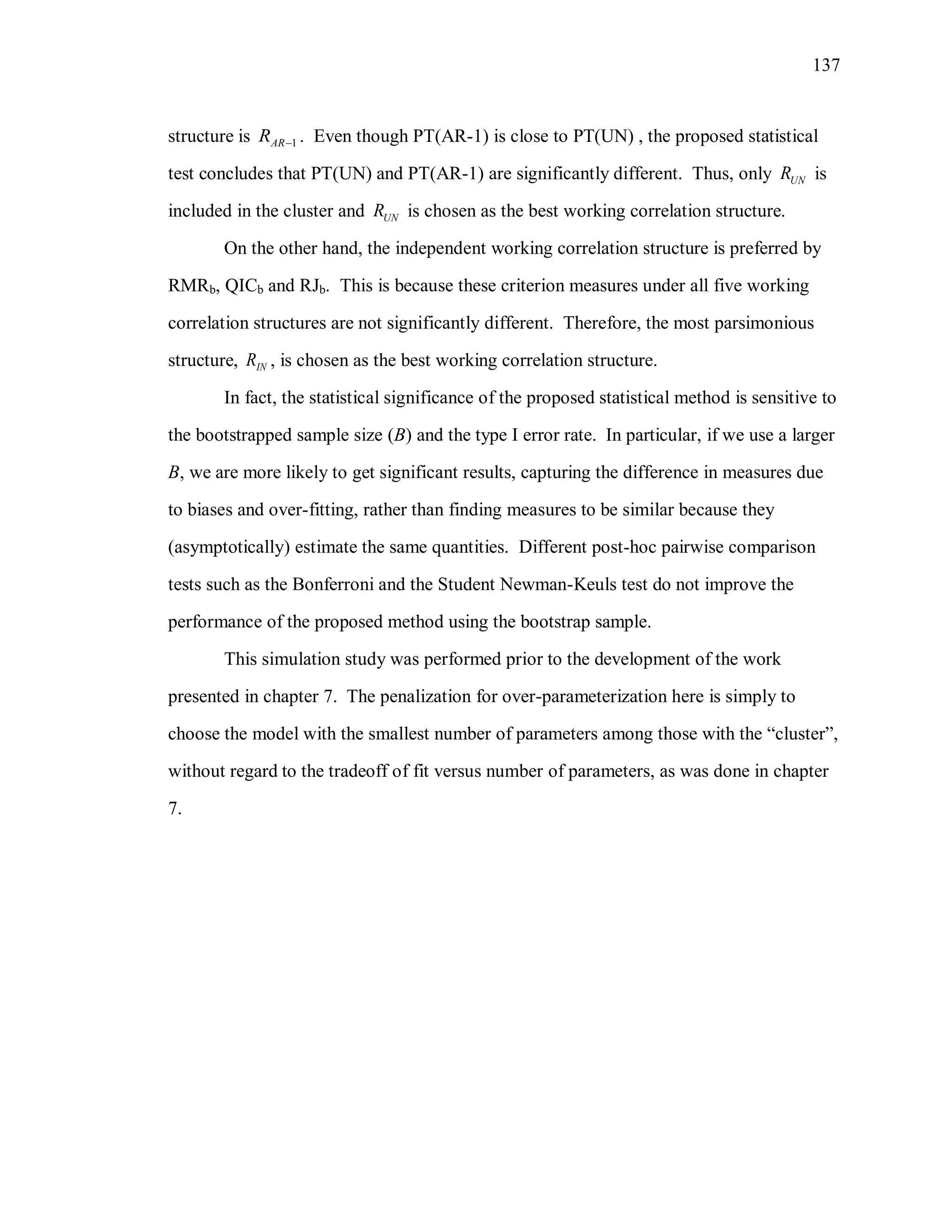
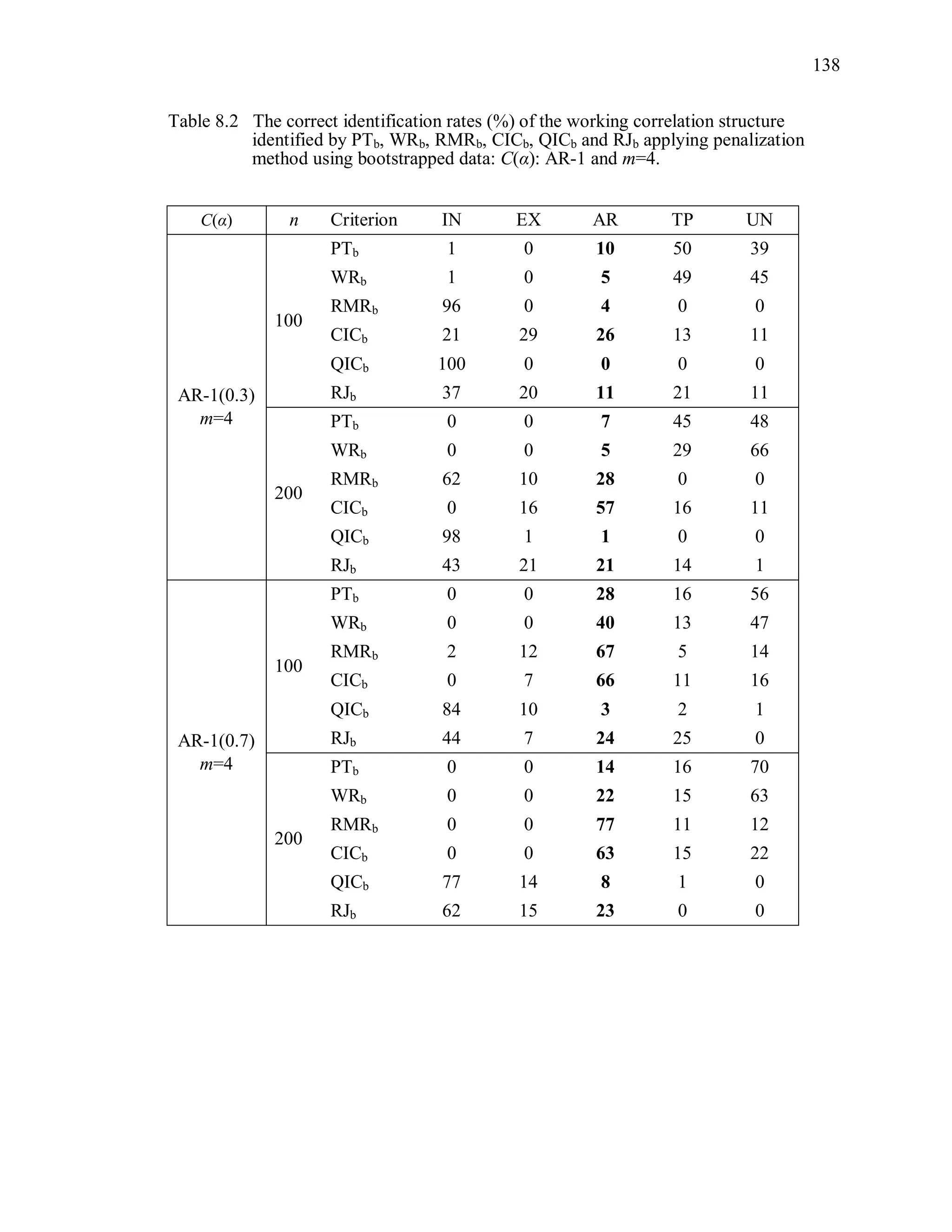
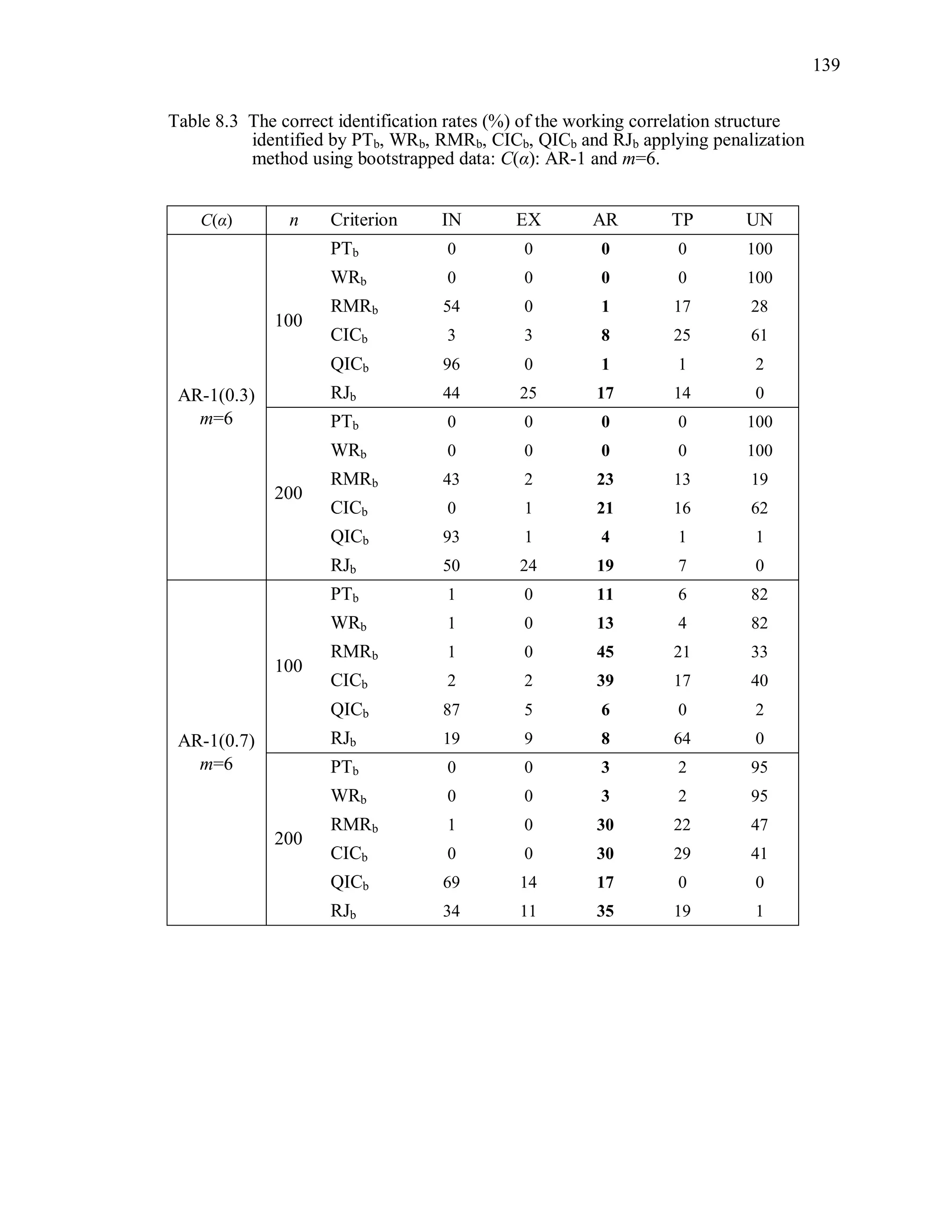
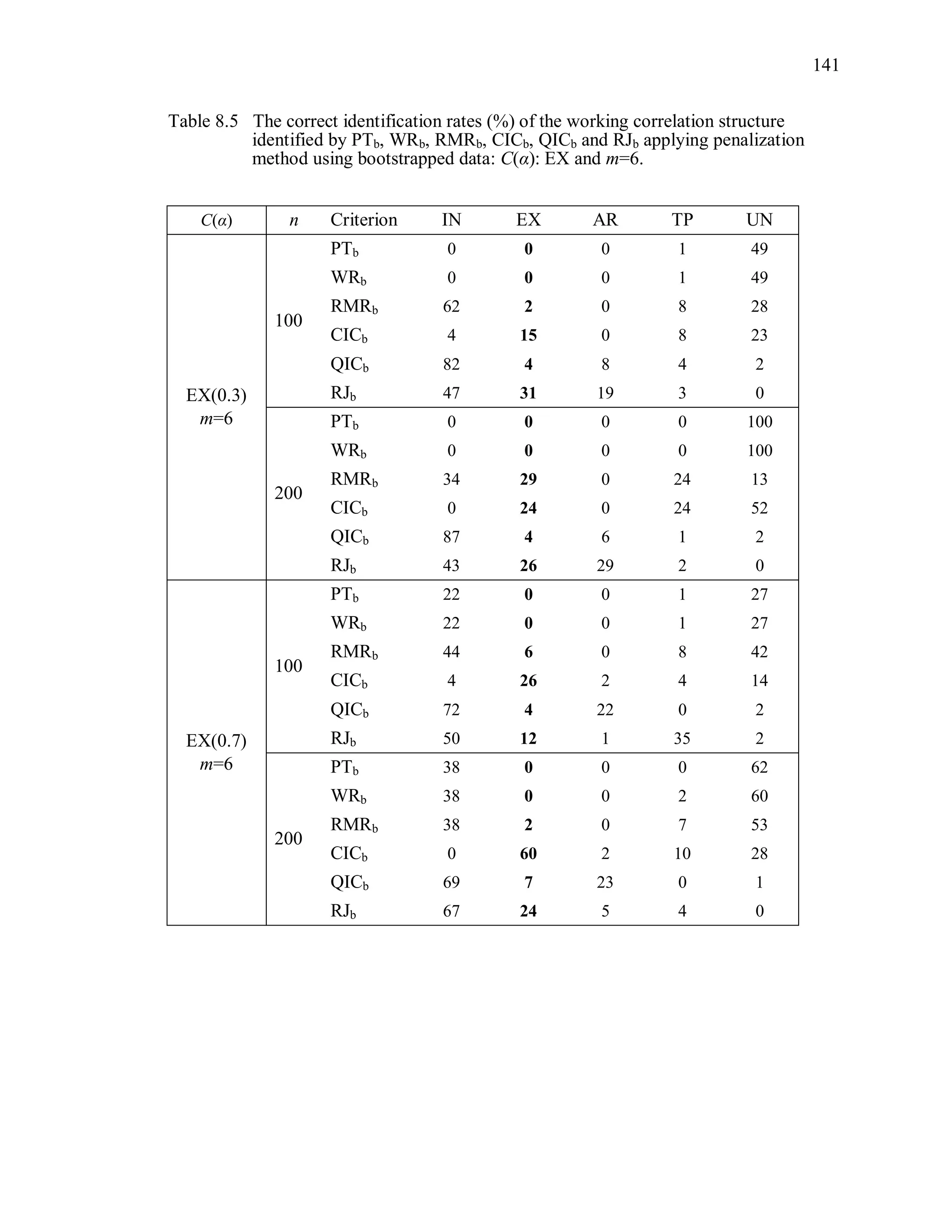
The simulation results reveal that the second penalization method using the
bootstrapped data is ineffective to improve the performance of PT, WR, RMR, CIC, QIC
and RJ (Table 8.2 ~ Table 8.5).
Over-parameterized structures are still preferred by PTb, WRb. Even though CICb
performs better than PTb, WRb, its overall correct identification rate is low even though
the sample size is large. Note that we expect that the criterion value under TR and the
criterion value under ovR will be “non-significantly” different. In other words, we expect
that TR and ovR will be included in the same cluster. However, the proposed statistical
test using the bootstrap sample tends to provide a significant difference between the two.
For instance, PT(UN) is the minimum among candidates when the true correlation

164. 137
structure is 1ARR  . Even though PT(AR-1) is close to PT(UN) , the proposed statistical
test concludes that PT(UN) and PT(AR-1) are significantly different. Thus, only UNR is
included in the cluster and UNR is chosen as the best working correlation structure.
On the other hand, the independent working correlation structure is preferred by
RMRb, QICb and RJb. This is because these criterion measures under all five working
correlation structures are not significantly different. Therefore, the most parsimonious
structure, INR , is chosen as the best working correlation structure.
In fact, the statistical significance of the proposed statistical method is sensitive to
the bootstrapped sample size (B) and the type I error rate. In particular, if we use a larger
B, we are more likely to get significant results, capturing the difference in measures due
to biases and over-fitting, rather than finding measures to be similar because they
(asymptotically) estimate the same quantities. Different post-hoc pairwise comparison
tests such as the Bonferroni and the Student Newman-Keuls test do not improve the
performance of the proposed method using the bootstrap sample.
This simulation study was performed prior to the development of the work
presented in chapter 7. The penalization for over-parameterization here is simply to
choose the model with the smallest number of parameters among those with the “cluster”,
without regard to the tradeoff of fit versus number of parameters, as was done in chapter
7.

165. 138
Table 8.2 The correct identification rates (%) of the working correlation structure
identified by PTb, WRb, RMRb, CICb, QICb and RJb applying penalization
method using bootstrapped data: C(α): AR-1 and m=4.
C(α) n Criterion IN EX AR TP UN
AR-1(0.3)
m=4
100
PTb 1 0 10 50 39
WRb 1 0 5 49 45
RMRb 96 0 4 0 0
CICb 21 29 26 13 11
QICb 100 0 0 0 0
RJb 37 20 11 21 11
200
PTb 0 0 7 45 48
WRb 0 0 5 29 66
RMRb 62 10 28 0 0
CICb 0 16 57 16 11
QICb 98 1 1 0 0
RJb 43 21 21 14 1
AR-1(0.7)
m=4
100
PTb 0 0 28 16 56
WRb 0 0 40 13 47
RMRb 2 12 67 5 14
CICb 0 7 66 11 16
QICb 84 10 3 2 1
RJb 44 7 24 25 0
200
PTb 0 0 14 16 70
WRb 0 0 22 15 63
RMRb 0 0 77 11 12
CICb 0 0 63 15 22
QICb 77 14 8 1 0
RJb 62 15 23 0 0

166. 139
Table 8.3 The correct identification rates (%) of the working correlation structure
identified by PTb, WRb, RMRb, CICb, QICb and RJb applying penalization
method using bootstrapped data: C(α): AR-1 and m=6.
C(α) n Criterion IN EX AR TP UN
AR-1(0.3)
m=6
100
PTb 0 0 0 0 100
WRb 0 0 0 0 100
RMRb 54 0 1 17 28
CICb 3 3 8 25 61
QICb 96 0 1 1 2
RJb 44 25 17 14 0
200
PTb 0 0 0 0 100
WRb 0 0 0 0 100
RMRb 43 2 23 13 19
CICb 0 1 21 16 62
QICb 93 1 4 1 1
RJb 50 24 19 7 0
AR-1(0.7)
m=6
100
PTb 1 0 11 6 82
WRb 1 0 13 4 82
RMRb 1 0 45 21 33
CICb 2 2 39 17 40
QICb 87 5 6 0 2
RJb 19 9 8 64 0
200
PTb 0 0 3 2 95
WRb 0 0 3 2 95
RMRb 1 0 30 22 47
CICb 0 0 30 29 41
QICb 69 14 17 0 0
RJb 34 11 35 19 1

167. 140
Table 8.4 The correct identification rates (%) of the working correlation structure
identified by PTb, WRb, RMRb, CICb, QICb and RJb applying penalization
method using bootstrapped data: C(α): EX and m=4.
C(α) n Criterion IN EX AR TP UN
EX(0.3)
m=4
100
PTb 0 0 0 17 33
WRb 0 0 0 16 34
RMRb 98 2 0 0 0
CICb 3 29 0 14 4
QICb 100 0 0 0 0
RJb 54 17 22 7 0
200
PTb 0 1 0 23 76
WRb 0 0 0 20 80
RMRb 85 12 0 2 1
CICb 1 64 0 17 18
QICb 96 1 3 0 0
RJb 59 18 21 2 0
EX(0.7)
m=4
100
PTb 0 4 0 19 27
WRb 0 4 0 25 21
RMRb 2 46 0 22 30
CICb 0 30 2 9 9
QICb 82 12 6 0 0
RJb 65 15 10 9 1
200
PTb 0 5 0 37 58
WRb 0 9 0 49 42
RMRb 0 45 0 23 32
CICb 0 58 0 21 21
QICb 73 8 19 0 0
RJb 68 19 12 1 0

168. 141
Table 8.5 The correct identification rates (%) of the working correlation structure
identified by PTb, WRb, RMRb, CICb, QICb and RJb applying penalization
method using bootstrapped data: C(α): EX and m=6.
C(α) n Criterion IN EX AR TP UN
EX(0.3)
m=6
100
PTb 0 0 0 1 49
WRb 0 0 0 1 49
RMRb 62 2 0 8 28
CICb 4 15 0 8 23
QICb 82 4 8 4 2
RJb 47 31 19 3 0
200
PTb 0 0 0 0 100
WRb 0 0 0 0 100
RMRb 34 29 0 24 13
CICb 0 24 0 24 52
QICb 87 4 6 1 2
RJb 43 26 29 2 0
EX(0.7)
m=6
100
PTb 22 0 0 1 27
WRb 22 0 0 1 27
RMRb 44 6 0 8 42
CICb 4 26 2 4 14
QICb 72 4 22 0 2
RJb 50 12 1 35 2
200
PTb 38 0 0 0 62
WRb 38 0 0 2 60
RMRb 38 2 0 7 53
CICb 0 60 2 10 28
QICb 69 7 23 0 1
RJb 67 24 5 4 0

169. 142
8.3 Conclusion
To penalize the over-parameterized working correlation structure, the two
different approaches have been proposed: (1) the cluster detection based on the spacings
of the order statistics of the criterion measure (chapter 7), and (2) the statistical test using
the bootstrapped data (chapter 8). These two approaches are developed based on the
similar motivations in which the true correlation structure and the over-parameterized
structure are expected to have relatively similar selection criterion values due to their
asymptotic properties, whereas those that are misspecified and cannot capture the
underlying correlation are biased and have larger values. Those candidate models with
similar values are considered clustered. Simulation results show that the first approach
can identify the cluster well, whereas the second approach does not do so even in large
samples. Moreover, the second approach is sensitive to several factors, including the
number of bootstrap samples taken. For penalizing the over-parameterized structure, the
first approach is recommended, as it incorporates a tradeoff between fit and the number
of parameters in the working correlation matrix more effectively than approach 2.

170. 143
CHAPTER 9
CONCLUSIONS AND FUTURE PLANS
We close this dissertation with a summary of contributions and several directions
for future work.
9.1 Conclusions
In this dissertation, a new selection criteria for working correlation structure in
GEE was developed based on generalized eigenvalues. A set of generalized eigenvalues
measures a disparity between the sandwich variance estimator under the hypothesized
working correlation matrix and the model-based variance estimator under working
independence assumption. A summary measure of the set of the generalized eigenvalues
provides an indication of the disparity between the true correlation structure and the
misspecified working correlation structure.
The proposed selection criteria use a bias-corrected sandwich variance estimator.
The use of a bias-corrected sandwich variance estimator mitigates the negative bias of the
sandwich variance estimator by Liang and Zeger (1986). Moreover, the use of a bias-
corrected sandwich variance estimator improves the correct identification rates of the
working correlation selection criteria. In this dissertation, four bias-corrected sandwich
variance estimators were described. Their impacts on selecting the most appropriate
working correlation structure were similar. Therefore, the simulation results using the
Wong and Long (2010) bias-correction method are presented in this dissertation.
Our simulation experiments show that the new selection criteria can distinguish
the true correlation matrix from the misspecified working correlation structure with high
success rates as the sample size increases. However, like other selection criterion
measures, they cannot distinguish the true underlying correlation matrix from the over-
parameterized structures. Therefore, we developed a method to penalize over-
parameterized structures h based on our cluster detection method and an optimization

171. 144
function that considers the trade-off between bias and variability. The simulation studies
suggest that the proposed penalization method greatly improves the performances of the
new selection criterion measures.
The GEE method is known to provide consistent regression parameter estimates
regardless of the choice of the working correlation structure if n consistent estimates of
nuisance parameters are used. In large samples, valid standard errors of the  estimates
can be obtained from the sandwich variance estimator. This dissertation focuses on the
statistical efficiency in small samples. The correct identification of the working
correlation structure improves the statistical efficiency, as was shown in chapter 3. In
that sense, our proposed working correlation selection criteria with the penalization for
the over-parameterized structure would contribute to the improvement of the statistical
efficiency in GEE.
9.2 Limitations and Future Directions
There are some limitations of this dissertation. A few suggestions for future
research is also discussed.
The proposed working correlation selection criteria are one-dimensional summary
measures of a set of generalized eigenvalues. One-dimensional summary measure loses
some information on the disparity between two covariance matrices in the multi-
dimensional space. Multivariate measures considering both direction and quantity of
each generalized eigenvalue might provide more information on the disparity between the
two covariance matrices.
The measures proposed are based upon the generalized eigenvalues of the
comparison of the sandwich estimator of the variance of the regression parameters under
a working correlation structure to the model-based estimator under independence. One
might intuitively think that a comparison of the sandwich estimator to the model-based
estimator both formed under the same working correlation would work to distinguish a

172. 145
good working model choice from a poor one. If the right choice was made, then both
should be measuring the same quantities and the generalized eigenvalues should all be
close to 1. However, in small sample sizes, both estimators still try to fit the model to the
data, and the sandwich estimator is not powerful enough to move far enough away from
the model-based estimator to signal a poor choice of the working correlation.
The derivation of the QIC and CIC motivates the use of these particular
generalized eigenvalues. But intuitively, we can appreciate that since the independence
structure has no correlation parameters and since the estimates themselves are not highly
influenced by the working correlation structure, the  elements of the variance matrix
( )M IN will tend to be pretty stable. Also, the higher the true correlations, the “larger” this
matrix will be, relative to the ideal T . So, in effect, we expect independence to be the
worst (but reasonably stable) choice, to which all others are compared.
In this dissertation, the marginal mean model and the variance function were
correctly specified to evaluate the performance of the criterion measures on the working
correlation structure selection. The effects of a misspecified or more complicated mean
structure (thus increasing the size of p) and the variance function on the working
correlation structure selection should be investigated.
Our simulation experiments used complete observations. Missing values are
common issues in the longitudinal data analysis. The impact of the missing data on the
working correlation structure selection should be investigated. Sparks (2009) proposed
the model selection criteria in a GLM framework based on the Kullback-Leiber
discrepancy that can be used in the presence of missing data. The criteria were developed
by accounting for missing data using principles related to the expectation maximization
(EM) algorithm and bootstrap methods. The approach taken by Sparks (2009) might be
helpful to improve the performance of our proposed working correlation selection criteria
in the presence of missing data.

173. 146
Our simulation experiments considered the five working correlation structures:
independence, exchangeable, AR-1, Toeplitz and unstructured matrices. They are
commonly used in many statistical packages. In principle, many types of user-specified
working correlation structure can be used. The performance of the proposed working
correlation selection criteria should be evaluated when other types of working correlation
structures are also considered.
In the modeling of the longitudinal data, the linear predictors, the link function,
the variance function and the working correlation structure must be chosen. QIC is a
widely used model selection criterion for the mean model and working correlation
structure, even though it has some limitations when used for working correlation
selection. Recently, several authors introduced other selection criteria for the covariate or
working correlation structure. Wang and Hin (2010) proposed the extended QIC (EQIC)
for the selection of the mean structure and variance function. Acion (2011) developed a
new model selection criteria based on Kullback-Leibler symmetric discrepancy and
demonstrated better performance than QIC. To our knowledge, there is no model
selection criterion identifying all three: the mean structure, the variance function and
working correlation structure, with high success rate. Combining our proposed working
correlation selection method with the recently developed other selection criteria, the
overall model selection strategies is planned for future research.
Finally, working to identify a better theoretical justification for the choice of an
optimization function that penalizes for over-parameterization is also part of future
research plans.

174. 147
APPENDIX A
RELATEIVE DIFFERENCE AND COVERAGE PROBABILITY OF
VARIANCE ESTIMATORS
Table A.1 Relative difference and coverage probability of each six variance estimator
(MB, LZ, MD, KC, Pan, WL) when the true correlation structure for the
binary responses is EX(0.3) and m=4.
Relative difference (%) Coverage probability (%)
IN EX AR-1 TOEP UN IN EX AR-1 TOEP UN
n=20
MB 1.9 -14.0 -19.3 -20.1 -28.6 93.4 93.2 90.2 91.3 89.5
LZ -5.3 -20.2 -14.7 -24.9 -31.2 91.9 92.1 91.9 90.5 87.3
MD 13.8 -6.7 0.7 -11.9 -18.4 94.4 93.6 93.4 92.3 90.4
KC 3.7 -13.8 -7.4 -18.7 -25.2 93.3 92.7 92.7 91.7 89.0
PAN 0.0 -16.1 -9.3 -20.7 -28.1 92.9 93.2 93.4 91.4 90.5
WL 1.9 -14.0 -19.3 -20.1 -28.6 93.4 93.2 90.2 91.3 89.5
n=40
MB 8.3 -11.7 -4.1 -16.4 -23.7 94.0 93.5 93.9 92.6 90.9
LZ 15.7 -2.2 -9.0 -5.4 -9.8 95.1 95.4 93.0 94.0 93.4
MD 12.7 -5.7 2.5 -8.8 -12.4 94.2 94.0 93.8 93.4 92.8
KC 23.5 1.9 11.2 -1.5 -5.1 95.3 94.7 95.1 94.2 93.1
PAN 18.0 -2.0 6.8 -5.3 -8.8 94.9 94.5 94.3 93.7 92.9
WL 14.7 -3.8 4.6 -6.9 -11.5 94.1 94.0 94.7 93.8 92.8
n=50
MB 19.2 -1.6 7.3 -4.7 -9.3 94.7 94.5 94.9 94.1 93.1
LZ 21.7 2.3 -5.4 -0.5 -4.6 95.7 95.8 93.5 95.3 94.6
MD 19.1 -0.7 7.8 -2.9 -6.7 94.7 95.5 94.3 94.6 93.8
KC 28.2 5.5 15.1 3.3 -0.6 95.5 95.6 94.9 95.6 94.9
PAN 23.6 2.3 11.4 0.1 -3.7 95.1 95.6 94.7 95.2 94.4
WL 22.7 2.4 12.1 -0.2 -4.2 95.4 95.4 95.1 93.9 93.5

175. 148
Table A.2 Relative difference and coverage probability of each six variance estimator
(MB, LZ, MD, KC, Pan, WL) when the true correlation structure for the
binary responses is EX(0.7) and m=4.
Relative difference (%) Coverage probability (%)
IN EX AR-1 TOEP UN IN EX AR-1 TOEP UN
n=20
MB 142.1 7.4 -22.2 -7.5 -22.8 97.0 95.8 87.6 92.2 90.5
LZ 127.4 -0.5 24.5 -9.7 -16.7 94.5 95.6 95.0 93.8 92.8
MD 181.0 16.0 48.9 6.5 2.3 96.5 96.9 97.2 95.8 95.3
KC 152.7 7.3 35.9 -2.8 -15.2 95.2 95.9 96.2 94.4 94.0
PAN 137.9 4.4 32.0 -5.2 -10.1 96.3 95.1 95.5 93.3 91.3
WL 142.1 7.4 -22.2 -7.5 -22.8 97.0 95.8 87.6 92.2 90.5
n=40
MB 165.2 9.7 40.4 0.4 36.8 97.3 96.3 96.4 94.5 92.9
LZ 134.0 0.0 -31.4 -8.4 -18.9 95.4 95.7 85.3 94.6 92.9
MD 128.3 -4.7 19.4 -9.7 -19.2 94.6 94.5 94.6 94.5 93.6
KC 153.5 2.7 30.3 -2.3 -12.3 95.5 95.5 95.7 95.5 94.8
PAN 140.5 -1.1 24.7 -6.2 -15.8 95.1 95.1 95.3 95.0 94.2
WL 137.7 -0.6 25.3 -6.5 -15.6 93.9 94.4 94.2 93.4 91.8
n=50
MB 150.6 1.7 29.0 -4.1 -13.2 94.9 94.5 94.5 93.7 92.2
LZ 140.3 3.6 -29.7 -3.0 -12.1 94.5 95.3 84.0 94.2 93.2
MD 140.7 0.5 27.0 -4.8 -11.2 93.7 94.6 93.8 93.2 93.7
KC 161.8 6.7 36.5 1.3 -5.3 94.7 95.5 94.7 94.4 94.1
PAN 151.0 3.5 31.6 -1.8 -9.1 94.2 95.0 94.3 93.9 93.8
WL 144.7 2.3 28.5 -2.5 -11.3 94.0 94.0 93.0 93.6 91.3

176. 149
Table A.3 Relative difference and coverage probability of each six variance estimator
(MB, LZ, MD, KC, Pan, WL) when the true correlation structure for the
binary responses is EX(0.3) and m=6.
Relative difference (%) Coverage probability (%)
IN EX AR-1 TOEP UN IN EX AR-1 TOEP UN
n=20
MB 15.4 -4.1 -16.0 -13.2 -33.6 95.5 96.1 91.5 92.8 84.5
LZ 9.3 -10.3 1.9 -17.1 -33.6 94.5 92.9 92.6 90.8 84.1
MD 28.8 2.7 18.0 -4.5 -22.1 96.3 94.7 94.7 93.0 88.0
KC 18.6 -4.0 9.6 -11.1 -28.2 95.5 94.2 93.7 92.0 86.2
PAN 14.7 -5.8 7.9 -12.4 -29.6 95.9 96.0 94.6 93.3 86.0
WL 15.4 -4.1 -16.0 -13.2 -33.6 95.5 96.1 91.5 92.8 84.5
n=40
MB 22.4 -2.4 12.4 -9.0 -26.1 96.9 96.3 95.0 94.1 87.1
LZ 16.7 -3.6 -17.2 -8.1 -17.9 95.0 95.0 90.3 94.2 92.3
MD 15.3 -7.3 7.7 -10.6 -19.9 93.8 93.3 92.9 92.4 91.5
KC 25.2 -0.9 15.7 -4.4 -14.1 95.0 94.4 94.0 93.3 92.4
PAN 20.1 -4.1 11.6 -7.6 -17.1 94.6 93.8 93.5 92.9 92.2
WL 18.2 -4.4 11.0 -8.3 -17.6 94.6 94.0 94.5 92.9 91.4
n=50
MB 22.0 -2.9 13.1 -6.7 -16.0 95.0 94.2 94.9 93.2 91.5
LZ 17.9 -2.9 -17.6 -6.2 -14.2 95.6 95.2 88.9 94.7 92.1
MD 17.8 -4.3 11.9 -7.5 -14.6 95.0 94.6 93.4 93.8 91.5
KC 25.8 0.9 18.6 -2.4 -9.7 96.0 95.0 94.4 94.2 92.4
PAN 21.7 -1.7 15.1 -4.9 -12.1 95.3 94.9 94.2 94.1 92.1
WL 20.2 -2.9 12.9 -6.0 -13.5 95.6 94.9 93.6 94.3 92.0

177. 150
Table A.4 Relative difference and coverage probability of each six variance estimator
(MB, LZ, MD, KC, Pan, WL) when the true correlation structure for the
binary responses is EX(0.7) and m=6.
Relative difference (%) Coverage probability (%)
IN EX AR-1 TOEP UN IN EX AR-1 TOEP UN
n=20
MB 142.1 7.8 -36.6 -8.6 -35.6 95.3 96.8 80.8 92.6 85.8
LZ 130.9 -1.0 44.1 2.7 -4.4 94.2 95.2 95.8 93.7 87.8
MD 180.4 12.7 67.7 29.5 26.1 96.3 96.9 97.4 95.4 91.0
KC 154.4 5.6 55.4 4.1 -2.5 95.4 96.0 96.9 94.6 89.5
PAN 145.4 5.7 53.5 6.7 5.8 95.8 96.6 96.5 94.6 88.6
WL 142.1 7.8 -36.6 -8.6 -35.6 95.3 96.8 80.8 92.6 85.8
n=40
MB 170.4 9.6 60.7 17.8 26.8 96.6 96.8 96.8 95.1 89.8
LZ 155.9 6.4 -42.9 -5.0 -27.4 96.4 95.6 78.4 92.9 89.2
MD 156.9 2.4 47.2 -2.0 -20.5 95.9 95.7 94.8 94.2 92.4
KC 182.9 9.2 58.6 5.0 -14.1 96.6 96.5 95.8 95.3 93.6
PAN 169.6 5.7 52.7 1.5 -19.3 96.2 96.1 95.4 94.6 93.3
WL 166.0 7.2 52.5 1.5 -15.4 96.3 94.8 93.8 93.1 89.7
n=50
MB 179.0 9.1 56.0 3.5 -12.9 96.7 95.1 93.8 93.2 90.2
LZ 133.8 -1.7 -47.6 -9.8 -27.4 94.6 94.1 75.5 93.2 91.2
MD 140.9 -3.7 35.8 -8.9 -23.7 94.8 94.2 94.5 93.2 91.9
KC 160.3 1.4 44.4 -3.8 -19.1 95.4 94.6 95.2 94.2 92.6
PAN 150.4 -1.2 39.9 -6.4 -21.5 95.1 94.3 94.9 93.7 92.4
WL 143.6 -3.2 37.7 -8.2 -24.8 94.7 93.7 94.5 93.2 90.0

178. 151
Table A.5 Relative difference and coverage probability of each six variance estimator
(MB, LZ, MD, KC, Pan, WL) when the true correlation structure for the
binary responses is TOEP and m=4.
Relative difference (%) Coverage probability (%)
IN EX AR-1 TOEP UN IN EX AR-1 TOEP UN
n=20
MB 34.0 10.4 7.0 -21.4 -27.5 95.1 94.2 92.3 91.3 89.2
LZ 24.8 2.7 18.9 -22.6 -28.5 93.2 93.1 93.3 92.7 89.1
MD 50.3 20.0 40.7 -7.0 -13.4 95.3 94.5 95.0 94.9 92.1
KC 36.9 10.9 29.2 -14.9 -21.2 94.3 93.6 94.1 93.9 90.7
PAN 31.2 7.4 25.4 -19.7 -26.3 95.0 93.8 94.1 92.9 91.0
WL 34.0 10.4 7.0 -21.4 -27.5 95.1 94.2 92.3 91.3 89.2
n=40
MB 42.4 13.0 33.1 -14.4 -21.1 95.5 94.6 94.7 94.0 91.8
LZ 39.2 15.2 11.4 -14.1 -17.3 95.0 95.4 91.4 93.7 92.9
MD 36.1 11.1 30.0 -15.0 -18.9 94.9 94.3 93.7 93.5 92.3
KC 49.3 19.9 41.2 -7.3 -11.5 95.1 95.2 94.8 95.4 93.7
PAN 42.5 15.4 35.5 -11.1 -15.2 95.0 94.5 94.6 94.5 93.1
WL 39.4 12.7 33.1 -12.9 -16.9 93.5 94.2 94.1 91.9 90.2
n=50
MB 45.0 15.3 36.7 -10.4 -14.5 94.3 94.3 94.3 92.6 90.7
LZ 48.9 22.4 17.6 -6.3 -9.1 94.6 95.1 92.6 94.0 93.9
MD 45.3 18.2 39.2 -6.7 -10.1 94.6 94.3 94.8 94.8 95.0
KC 56.4 25.6 48.7 -0.1 -3.6 95.4 95.2 95.3 95.5 95.6
PAN 50.7 21.9 43.9 -3.5 -6.9 95.2 94.7 95.1 95.1 95.3
WL 48.8 21.7 43.1 -6.3 -9.6 94.6 94.6 94.6 93.3 93.5

179. 152
Table A.6 Relative difference and coverage probability of each six variance estimator
(MB, LZ, MD, KC, Pan, WL) when the true correlation structure for the
binary responses is TOEP and m=6.
Relative difference (%) Coverage probability (%)
IN EX AR-1 TOEP UN IN EX AR-1 TOEP UN
n=20
MB 68.4 33.3 16.1 -19.3 -38.4 95.7 96.1 90.3 92.3 85.5
LZ 59.5 24.5 60.9 -11.7 -25.0 94.5 94.3 94.4 93.1 88.5
MD 88.6 42.3 86.4 4.0 -7.6 95.5 95.7 95.9 95.3 90.8
KC 73.4 33.1 73.1 -6.4 -25.4 95.2 94.9 95.3 94.3 89.5
PAN 68.1 30.0 67.3 -9.7 -14.8 94.9 94.8 94.5 93.0 85.6
WL 68.4 33.3 16.1 -19.3 -38.4 95.7 96.1 90.3 92.3 85.5
n=40
MB 80.2 34.6 74.6 -5.2 -6.0 95.6 95.2 94.6 93.5 86.6
LZ 72.8 34.4 10.1 -15.1 -27.9 93.5 94.7 85.5 92.4 90.8
MD 71.9 31.0 75.6 -12.6 -23.0 92.1 94.1 94.1 91.7 90.7
KC 86.9 40.0 88.7 -5.9 -16.7 93.6 94.8 95.2 92.8 92.1
PAN 79.2 35.4 82.0 -9.3 -20.5 92.6 94.5 94.6 92.4 91.3
WL 75.3 35.0 78.7 -9.4 -21.1 92.8 93.3 93.5 92.3 90.5
n=50
MB 81.2 37.1 82.2 -7.6 -19.2 93.4 93.4 93.9 93.0 91.0
LZ 81.9 42.4 17.8 -8.7 -19.8 94.3 95.1 85.6 93.5 91.3
MD 81.2 37.7 82.9 -8.4 -17.5 93.6 93.6 92.7 93.3 91.1
KC 93.7 45.2 93.8 -3.0 -12.2 94.0 94.2 93.5 93.6 93.0
PAN 87.3 41.4 88.3 -5.8 -15.7 93.6 94.1 93.1 93.4 91.6
WL 84.4 40.5 87.6 -5.5 -14.0 94.3 93.9 93.3 93.1 91.0

180. 153
Table A.7 Relative difference and coverage probability of each six variance estimator
(MB, LZ, MD, KC, Pan, WL) when the true correlation structure for the
binary responses is UN and m=4.
Relative difference (%) Coverage probability (%)
IN EX AR-1 TOEP UN IN EX AR-1 TOEP UN
n=20
MB 104.2 46.6 20.9 12.5 -25.2 95.2 95.4 93.7 91.7 90.3
LZ 89.8 34.0 11.3 10.6 -28.5 92.8 93.5 92.5 90.8 89.8
MD 130.6 56.5 31.0 31.1 -13.0 94.9 95.5 94.9 93.7 92.3
KC 109.0 44.7 20.6 20.3 -23.7 93.8 94.8 94.0 92.6 91.0
PAN 20.7 -1.2 15.4 -26.1 -32.3 95.0 93.8 94.1 92.9 91.0
WL 104.2 46.6 20.9 12.5 -25.2 95.2 95.4 93.7 91.7 90.3
n=40
MB 31.0 3.9 22.4 -21.3 -27.4 95.5 94.6 94.7 94.0 91.8
LZ 99.7 43.2 18.0 13.7 -21.3 94.9 95.7 94.9 94.1 92.1
MD 95.6 37.1 13.8 14.6 -22.0 93.5 94.4 93.2 92.8 93.3
KC 115.3 47.9 23.3 24.4 -14.4 94.0 95.6 95.1 94.1 94.2
PAN 105.2 42.3 18.5 19.4 -18.2 93.7 95.3 94.4 93.8 93.5
WL 38.2 11.7 31.9 -13.6 -17.7 93.5 94.2 94.1 91.9 90.2
n=50
MB 43.8 14.3 35.5 -11.2 -15.3 94.3 94.3 94.3 92.6 90.7
LZ 108.3 47.5 21.0 18.5 -17.8 95.3 95.0 94.2 93.1 92.6
MD 105.4 43.5 19.3 20.0 -15.4 94.5 93.9 94.5 93.3 93.9
KC 121.7 52.5 27.2 28.1 -9.0 95.5 95.3 95.2 94.0 94.8
PAN 113.4 47.9 23.2 23.9 -12.6 95.1 94.8 95.0 93.8 94.4
WL 46.4 19.7 40.8 -7.8 -11.0 94.6 94.6 94.6 93.3 93.5

181. 154
Table A.8 Relative difference and coverage probability of each six variance estimator
(MB, LZ, MD, KC, Pan, WL) when the true correlation structure for the
binary responses is UN and m=6.
Relative difference (%) Coverage probability (%)
IN EX AR-1 TOEP UN IN EX AR-1 TOEP UN
n=20
MB 47.9 21.7 -3.4 -2.3 -41.6 95.6 95.8 93.5 92.8 84.4
LZ 41.8 14.9 3.5 -5.3 -33.1 93.2 93.4 92.7 90.5 84.8
MD 67.3 31.5 19.5 9.2 -18.1 94.9 94.7 94.2 91.8 88.3
KC 53.9 22.9 11.2 1.7 -33.5 94.0 93.6 93.2 91.4 86.1
PAN 51.5 17.2 50.8 -18.6 -23.2 94.9 94.8 94.5 93.0 85.6
WL 47.9 21.7 -3.4 -2.3 -41.6 95.6 95.8 93.5 92.8 84.4
n=40
MB 47.9 21.7 -3.4 -2.3 -41.6 95.6 95.8 93.5 92.8 84.4
LZ 41.8 14.9 3.5 -5.3 -33.1 93.2 93.4 92.7 90.5 84.8
MD 67.3 31.5 19.5 9.2 -18.1 94.9 94.7 94.2 91.8 88.3
KC 53.9 22.9 11.2 1.7 -33.5 94.0 93.6 93.2 91.4 86.1
PAN 51.5 17.2 50.8 -18.6 -23.2 94.9 94.8 94.5 93.0 85.6
WL 47.9 21.7 -3.4 -2.3 -41.6 95.6 95.8 93.5 92.8 84.4
n=50
MB 80.7 36.6 81.6 -7.9 -19.5 93.4 93.4 93.9 93.0 91.0
LZ 74.3 42.6 11.5 19.6 -23.4 95.8 95.6 93.8 94.7 90.1
MD 73.5 38.3 24.4 18.0 -21.7 95.0 94.5 94.9 94.6 91.7
KC 85.3 45.8 31.6 24.7 -16.5 95.6 95.0 95.5 95.6 92.5
PAN 79.2 42.0 27.9 21.3 -19.7 95.4 94.7 95.4 94.9 92.0
WL 76.8 34.7 79.8 -9.4 -17.6 94.3 93.9 93.3 93.1 91.0

182. 155
Table A.9 Monte Carlo variance of the variance estimators: Correlated binary responses,
C(α): AR-1(0.3), m=4
Monte Carlo variance of the variance estimators
IN EX AR-1 TOEP UN
n=20
MB 0.066 0.071 0.080 0.081 0.088
LZ 0.217 0.219 0.211 0.201 0.213
MD 0.261 0.282 0.259 0.265 0.285
KC 0.234 0.249 0.239 0.239 0.238
PAN 0.077 0.079 0.085 0.080 0.087
WL 0.089 0.090 0.093 0.090 0.098
n=40
MB 0.006 0.007 0.008 0.008 0.008
LZ 0.024 0.024 0.024 0.023 0.023
MD 0.030 0.029 0.029 0.029 0.029
KC 0.027 0.026 0.027 0.026 0.026
PAN 0.007 0.007 0.008 0.008 0.008
WL 0.008 0.008 0.008 0.008 0.009
n=50
MB 0.003 0.003 0.004 0.004 0.004
LZ 0.011 0.012 0.012 0.011 0.012
MD 0.013 0.014 0.013 0.013 0.013
KC 0.012 0.013 0.012 0.012 0.012
PAN 0.004 0.004 0.004 0.004 0.004
WL 0.004 0.004 0.004 0.004 0.004

183. 156
Table A.10 Monte Carlo variance of the variance estimators: Correlated binary responses,
C(α): AR-1(0.7), m=4
Monte Carlo variance of the variance estimators
IN EX AR-1 TOEP UN
n=20
MB 0.092 0.095 0.081 0.074 0.069
LZ 0.210 0.185 0.136 0.131 0.158
MD 0.253 0.254 0.192 0.188 0.221
KC 0.231 0.222 0.165 0.155 0.187
PAN 0.136 0.101 0.071 0.069 0.091
WL 0.152 0.112 0.079 0.077 0.103
n=40
MB 0.007 0.009 0.008 0.006 0.007
LZ 0.026 0.020 0.014 0.013 0.015
MD 0.034 0.025 0.017 0.017 0.019
KC 0.030 0.022 0.016 0.015 0.017
PAN 0.013 0.009 0.006 0.006 0.009
WL 0.014 0.009 0.007 0.006 0.010
n=50
MB 0.003 0.004 0.003 0.003 0.003
LZ 0.012 0.010 0.007 0.006 0.007
MD 0.015 0.011 0.008 0.007 0.009
KC 0.013 0.011 0.007 0.007 0.007
PAN 0.007 0.005 0.003 0.003 0.004
WL 0.008 0.005 0.003 0.003 0.004

184. 157
Table A.11 Monte Carlo variance of the variance estimators: Correlated binary responses,
C(α): AR-1(0.3), m=6
Monte Carlo variance of the variance estimators
IN EX AR-1 TOEP UN
n=20
MB 0.015 0.016 0.020 0.020 0.022
LZ 0.079 0.077 0.071 0.066 0.063
MD 0.112 0.106 0.099 0.093 0.094
KC 0.094 0.090 0.084 0.078 0.076
PAN 0.020 0.021 0.020 0.020 0.024
WL 0.023 0.023 0.022 0.022 0.026
n=40
MB 0.002 0.002 0.002 0.002 0.002
LZ 0.010 0.010 0.009 0.009 0.009
MD 0.012 0.012 0.011 0.011 0.010
KC 0.011 0.011 0.010 0.010 0.010
PAN 0.002 0.002 0.002 0.002 0.003
WL 0.002 0.002 0.002 0.002 0.003
n=50
MB 0.001 0.001 0.001 0.001 0.001
LZ 0.005 0.005 0.005 0.005 0.004
MD 0.006 0.005 0.005 0.005 0.005
KC 0.005 0.005 0.005 0.005 0.005
PAN 0.001 0.001 0.001 0.001 0.001
WL 0.001 0.001 0.001 0.001 0.001

185. 158
Table A.12 Monte Carlo variance of the variance estimators: Correlated binary responses,
C(α): AR-1(0.7), m=6
Monte Carlo variance of the variance estimators
IN EX AR-1 TOEP UN
n=20
MB 0.019 0.023 0.017 0.014 0.042
LZ 0.097 0.072 0.034 0.037 0.086
MD 0.146 0.099 0.047 0.045 0.112
KC 0.119 0.084 0.039 0.044 0.087
PAN 0.038 0.029 0.016 0.017 0.067
WL 0.047 0.031 0.018 0.019 0.074
n=40
MB 0.002 0.003 0.002 0.002 0.002
LZ 0.012 0.009 0.005 0.004 0.010
MD 0.015 0.010 0.005 0.005 0.013
KC 0.014 0.010 0.005 0.005 0.006
PAN 0.004 0.003 0.002 0.001 0.002
WL 0.005 0.003 0.002 0.002 0.003
n=50
MB 0.001 0.001 0.001 0.001 0.001
LZ 0.006 0.004 0.002 0.002 0.002
MD 0.007 0.005 0.003 0.002 0.003
KC 0.007 0.005 0.002 0.002 0.003
PAN 0.002 0.002 0.001 0.001 0.001
WL 0.002 0.002 0.001 0.001 0.001

186. 159
Table A.13 Monte Carlo variance of the variance estimators: Correlated binary responses,
C(α): EX(0.3), m=4
Monte Carlo variance of the variance estimators
IN EX AR-1 TOEP UN
n=20
MB 0.073 0.084 0.113 0.089 0.099
LZ 0.232 0.219 0.263 0.217 0.228
MD 0.287 0.290 0.308 0.285 0.292
KC 0.250 0.247 0.283 0.246 0.257
PAN 0.087 0.086 0.100 0.088 0.103
WL 0.104 0.098 0.115 0.100 0.113
n=40
MB 0.006 0.008 0.012 0.008 0.008
LZ 0.025 0.024 0.028 0.023 0.023
MD 0.031 0.028 0.035 0.028 0.029
KC 0.028 0.026 0.031 0.025 0.026
PAN 0.008 0.008 0.009 0.008 0.009
WL 0.009 0.009 0.009 0.009 0.009
n=50
MB 0.003 0.004 0.006 0.004 0.004
LZ 0.011 0.012 0.015 0.012 0.012
MD 0.013 0.014 0.018 0.014 0.014
KC 0.012 0.013 0.017 0.013 0.013
PAN 0.004 0.004 0.004 0.004 0.004
WL 0.004 0.004 0.005 0.004 0.005

187. 160
Table A.14 Monte Carlo variance of the variance estimators: Correlated binary responses,
C(α): EX(0.7), m=4
Monte Carlo variance of the variance estimators
IN EX AR-1 TOEP UN
n=20
MB 0.071 0.060 0.053 0.062 0.071
LZ 0.220 0.132 0.243 0.134 0.124
MD 0.262 0.193 0.340 0.196 0.180
KC 0.249 0.159 0.287 0.160 0.138
PAN 0.135 0.060 0.126 0.064 0.074
WL 0.166 0.067 0.142 0.071 0.079
n=40
MB 0.008 0.007 0.005 0.008 0.008
LZ 0.029 0.017 0.033 0.018 0.018
MD 0.037 0.020 0.042 0.022 0.022
KC 0.033 0.018 0.037 0.020 0.020
PAN 0.016 0.007 0.015 0.008 0.013
WL 0.018 0.007 0.016 0.008 0.014
n=50
MB 0.004 0.003 0.002 0.004 0.004
LZ 0.014 0.008 0.017 0.008 0.012
MD 0.018 0.009 0.020 0.009 0.013
KC 0.016 0.009 0.018 0.009 0.009
PAN 0.008 0.003 0.007 0.003 0.004
WL 0.009 0.003 0.007 0.003 0.004

188. 161
Table A.15 Monte Carlo variance of the variance estimators: Correlated binary responses,
C(α): EX(0.3), m=6
Monte Carlo variance of the variance estimators
IN EX AR-1 TOEP UN
n=20
MB 0.018 0.023 0.043 0.024 0.030
LZ 0.086 0.076 0.100 0.074 0.080
MD 0.125 0.104 0.143 0.103 0.105
KC 0.104 0.089 0.119 0.087 0.091
PAN 0.026 0.025 0.032 0.028 0.041
WL 0.031 0.027 0.035 0.031 0.046
n=40
MB 0.002 0.002 0.006 0.003 0.003
LZ 0.011 0.009 0.012 0.009 0.009
MD 0.013 0.011 0.015 0.010 0.010
KC 0.012 0.010 0.013 0.010 0.010
PAN 0.003 0.002 0.003 0.002 0.003
WL 0.003 0.002 0.003 0.002 0.003
n=50
MB 0.001 0.001 0.002 0.001 0.001
LZ 0.006 0.005 0.007 0.005 0.004
MD 0.007 0.006 0.008 0.005 0.005
KC 0.006 0.005 0.008 0.005 0.005
PAN 0.001 0.001 0.002 0.001 0.001
WL 0.001 0.001 0.002 0.001 0.001

189. 162
Table A.16 Monte Carlo variance of the variance estimators: Correlated binary responses,
C(α): EX(0.7), m=6
Monte Carlo variance of the variance estimators
IN EX AR-1 TOEP UN
n=20
MB 0.0223 0.0213 0.0129 0.0269 0.0379
LZ 0.1015 0.0503 0.1182 0.0621 0.0850
MD 0.1577 0.0678 0.1713 0.0832 0.0970
KC 0.1262 0.0583 0.1418 0.0676 0.0826
PAN 0.0535 0.0219 0.0608 0.0272 0.0844
WL 0.0683 0.0236 0.0672 0.0320 0.0856
n=40
MB 0.0026 0.0018 0.0009 0.0020 0.0020
LZ 0.0123 0.0046 0.0147 0.0055 0.0095
MD 0.0153 0.0054 0.0176 0.0066 0.0120
KC 0.0137 0.0050 0.0161 0.0060 0.0060
PAN 0.0066 0.0020 0.0056 0.0025 0.0123
WL 0.0075 0.0021 0.0058 0.0026 0.0045
n=50
MB 0.0011 0.0009 0.0004 0.0010 0.0011
LZ 0.0059 0.0028 0.0075 0.0028 0.0026
MD 0.0071 0.0031 0.0088 0.0032 0.0030
KC 0.0065 0.0029 0.0081 0.0030 0.0028
PAN 0.0031 0.0010 0.0029 0.0010 0.0013
WL 0.0034 0.0010 0.0030 0.0010 0.0013

190. 163
Table A.17 Monte Carlo variance of the variance estimators: Correlated binary responses,
C(α): TOEP, m=4
Monte Carlo variance of the variance estimators
IN EX AR-1 TOEP UN
n=20
MB 0.070 0.078 0.123 0.113 0.099
LZ 0.221 0.207 0.255 0.229 0.217
MD 0.264 0.271 0.310 0.328 0.300
KC 0.240 0.236 0.282 0.279 0.264
PAN 0.093 0.088 0.098 0.110 0.109
WL 0.108 0.099 0.111 0.124 0.124
n=40
MB 0.006 0.008 0.015 0.013 0.012
LZ 0.025 0.024 0.030 0.030 0.028
MD 0.031 0.029 0.037 0.038 0.036
KC 0.028 0.026 0.033 0.034 0.031
PAN 0.009 0.009 0.009 0.011 0.011
WL 0.010 0.009 0.010 0.012 0.011
n=50
MB 0.003 0.004 0.007 0.006 0.006
LZ 0.012 0.012 0.015 0.016 0.015
MD 0.014 0.014 0.018 0.020 0.019
KC 0.013 0.013 0.017 0.018 0.017
PAN 0.004 0.004 0.004 0.005 0.005
WL 0.005 0.005 0.005 0.006 0.005

191. 164
Table A.18 Monte Carlo variance of the variance estimators: Correlated binary responses,
C(α): TOEP, m=6
Monte Carlo variance of the variance estimators
IN EX AR-1 TOEP UN
n=20
MB 0.019 0.023 0.059 0.022 0.028
LZ 0.086 0.072 0.109 0.061 0.076
MD 0.123 0.098 0.152 0.091 0.101
KC 0.105 0.084 0.130 0.074 0.077
PAN 0.030 0.026 0.034 0.027 0.065
WL 0.036 0.028 0.037 0.031 0.078
n=40
MB 0.002 0.002 0.007 0.002 0.003
LZ 0.010 0.008 0.016 0.006 0.008
MD 0.013 0.010 0.019 0.008 0.010
KC 0.011 0.009 0.017 0.007 0.008
PAN 0.003 0.003 0.004 0.002 0.004
WL 0.003 0.003 0.004 0.002 0.004
n=50
MB 0.001 0.001 0.004 0.001 0.001
LZ 0.005 0.004 0.007 0.003 0.005
MD 0.006 0.005 0.009 0.004 0.006
KC 0.005 0.005 0.008 0.003 0.004
PAN 0.001 0.001 0.002 0.001 0.001
WL 0.002 0.001 0.002 0.001 0.001

192. 165
Table A.19 Monte Carlo variance of the variance estimators: Correlated binary responses,
C(α): UN, m=4
Monte Carlo variance of the variance estimators
IN EX AR-1 TOEP UN
n=20
MB 0.068 0.079 0.072 0.067 0.068
LZ 0.207 0.180 0.152 0.144 0.140
MD 0.267 0.257 0.217 0.202 0.205
KC 0.239 0.216 0.184 0.176 0.164
PAN 0.093 0.088 0.098 0.110 0.109
WL 0.108 0.099 0.111 0.124 0.124
n=40
MB 0.007 0.008 0.008 0.007 0.009
LZ 0.025 0.023 0.018 0.018 0.020
MD 0.032 0.027 0.022 0.022 0.025
KC 0.028 0.025 0.020 0.020 0.022
PAN 0.009 0.009 0.009 0.011 0.011
WL 0.010 0.009 0.010 0.012 0.011
n=50
MB 0.003 0.004 0.004 0.003 0.005
LZ 0.013 0.011 0.010 0.009 0.012
MD 0.016 0.013 0.012 0.011 0.015
KC 0.014 0.012 0.011 0.010 0.013
PAN 0.004 0.004 0.004 0.005 0.005
WL 0.005 0.005 0.005 0.006 0.005

193. 166
Table A.20 Monte Carlo variance of the variance estimators: Correlated binary responses,
C(α): UN, m=6
Monte Carlo variance of the variance estimators
IN EX AR-1 TOEP UN
n=20
MB 0.017 0.021 0.026 0.021 0.044
LZ 0.087 0.074 0.077 0.061 0.082
MD 0.127 0.102 0.109 0.084 0.110
KC 0.105 0.087 0.091 0.072 0.079
PAN 0.030 0.026 0.034 0.027 0.065
WL 0.036 0.028 0.037 0.031 0.078
n=40
MB 0.002 0.002 0.003 0.002 0.004
LZ 0.011 0.009 0.008 0.007 0.016
MD 0.013 0.010 0.010 0.008 0.022
KC 0.012 0.010 0.009 0.008 0.013
PAN 0.003 0.003 0.004 0.002 0.004
WL 0.003 0.003 0.004 0.002 0.004
n=50
MB 0.001 0.001 0.001 0.001 0.002
LZ 0.006 0.005 0.005 0.004 0.005
MD 0.006 0.005 0.005 0.004 0.006
KC 0.006 0.005 0.005 0.004 0.005
PAN 0.001 0.001 0.002 0.001 0.001
WL 0.002 0.001 0.002 0.001 0.001

194. 167
APPENDIX B
THE PERFORMANCE OF THE CRITERIA WITHOUT
PENALIZATION FOR OVER-PARAMETERIZED STRUCTURES
Table B.1 Frequencies of the working correlation structure identified by PT, WR, RMR,
CIC, QIC and RJ from 1000 independent replications:
Correlated binary response; C(α): AR-1(0.3), m=4
n Criterion Wc1={IN, EX, AR-1} Wc2={IN, EX, AR-1,TOEP, UN}
IN EX AR-1 IN EX AR-1 TOEP UN
20
PT 15 217 768 8 26 78 153 735
WR 14 216 770 8 24 77 155 736
RMR 112 233 655 38 25 42 88 807
CIC 118 222 660 44 64 117 172 603
QIC 304 250 446 171 115 129 191 394
RJ 293 389 318 12 210 375 139 264
30
PT 3 168 829 2 11 33 93 861
WR 2 168 830 1 12 29 95 863
RMR 84 201 715 26 26 30 70 848
CIC 80 187 733 34 40 89 149 688
QIC 298 224 478 196 122 123 165 394
RJ 217 467 316 2 222 368 155 253
50
PT 0 118 882 0 1 16 75 908
WR 0 120 880 0 0 18 75 907
RMR 71 173 756 28 9 43 50 870
CIC 39 187 774 19 46 83 130 722
QIC 288 246 466 206 139 136 148 371
RJ 146 489 365 1 268 371 126 234
100
PT 0 58 942 0 0 7 40 953
WR 0 56 944 0 0 8 41 951
RMR 24 118 858 2 6 21 39 932
CIC 4 106 890 0 23 106 136 735
QIC 315 245 440 250 194 136 108 312
RJ 36 570 394 0 287 367 135 211
200
PT 0 9 991 0 0 0 40 960
WR 0 10 990 0 0 0 42 958
RMR 5 52 943 2 0 15 45 938
CIC 1 48 951 0 6 99 154 741
QIC 282 253 465 247 209 131 104 309
RJ 5 600 395 0 294 393 139 174

195. 168
Table B.2 Frequencies of the working correlation structure identified by PT, WR, RMR,
CIC, QIC and RJ from 1000 independent replications:
Correlated binary response; C(α): AR-1(0.6), m=4
n Criterion
Wc1={IN, EX, AR-1} Wc2={IN, EX, AR-1,TOEP, UN}
IN EX AR-1 IN EX AR-1 TOEP UN
20
PT 43 145 812 35 55 197 209 504
WR 43 144 813 35 56 200 203 506
RMR 39 184 777 15 24 83 150 728
CIC 56 192 752 42 96 210 224 428
QIC 304 263 433 240 169 139 204 248
RJ 89 551 360 35 278 348 129 210
30
PT 3 81 916 2 27 90 149 732
WR 3 76 921 2 28 92 148 730
RMR 14 110 876 7 11 62 131 789
CIC 4 150 846 2 59 132 226 581
QIC 308 264 428 264 196 109 158 273
RJ 6 590 404 2 309 357 112 220
50
PT 6 37 957 5 11 73 118 793
WR 6 35 959 5 11 76 120 788
RMR 14 83 903 7 10 68 136 779
CIC 6 86 908 5 25 141 219 610
QIC 292 258 450 244 194 114 167 281
RJ 8 590 402 5 306 358 113 218
100
PT 0 5 995 0 3 28 78 891
WR 0 5 995 0 3 25 74 898
RMR 2 32 966 1 1 75 139 784
CIC 0 35 965 0 6 133 164 697
QIC 328 268 404 283 225 99 130 263
RJ 0 586 414 0 340 338 125 197
200
PT 0 0 1000 0 0 26 62 912
WR 0 0 1000 0 0 19 65 916
RMR 0 5 995 0 0 71 129 800
CIC 0 2 998 0 0 108 193 699
QIC 314 254 432 287 228 130 117 238
RJ 0 621 379 0 308 393 116 183

196. 169
Table B.3 Frequencies of the working correlation structure identified by PT, WR, RMR,
CIC, QIC and RJ from 1000 independent replications:
Correlated binary response; C(α): AR-1(0.3), m=6
n Criterion
Wc1={IN, EX, AR-1} Wc2={IN, EX, AR-1,TOEP, UN}
IN EX AR-1 IN EX AR-1 TOEP UN
20
PT 6 130 864 1 5 64 215 715
WR 6 129 865 0 5 64 215 716
RMR 94 245 661 4 8 14 38 936
CIC 105 191 704 19 24 71 204 682
QIC 293 234 473 150 101 134 249 366
RJ 234 428 338 3 199 416 177 205
30
PT 0 45 955 0 1 19 77 903
WR 0 46 954 0 1 20 76 903
RMR 62 183 755 8 7 8 20 957
CIC 52 148 800 11 12 44 109 824
QIC 285 233 482 143 118 105 169 465
RJ 144 484 372 0 202 385 158 255
50
PT 0 40 960 0 0 5 9 986
WR 0 39 961 0 0 5 11 984
RMR 41 171 788 4 4 3 6 983
CIC 34 113 853 4 13 28 58 897
QIC 312 219 469 193 108 116 135 448
RJ 95 545 360 0 249 367 141 243
100
PT 0 5 995 0 0 0 2 998
WR 0 4 996 0 0 0 2 998
RMR 10 132 858 0 0 5 4 991
CIC 7 55 938 0 7 32 47 914
QIC 312 233 455 211 147 120 127 395
RJ 20 561 419 0 265 384 137 214
200
PT 0 0 1000 0 0 0 3 997
WR 0 0 1000 0 0 0 3 997
RMR 0 73 927 0 0 2 3 995
CIC 2 12 986 1 0 29 80 890
QIC 326 243 431 243 176 120 123 338
RJ 6 604 390 0 301 391 155 153

197. 170
Table B.4 Frequencies of the working correlation structure identified by PT, WR, RMR,
CIC, QIC and RJ from 1000 independent replications:
Correlated binary response; C(α): AR-1(0.6), m=6
n Criterion
Wc1={IN, EX, AR-1} Wc2={IN, EX, AR-1,TOEP, UN}
IN EX AR-1 IN EX AR-1 TOEP UN
20
PT 5 84 911 5 31 134 334 496
WR 5 80 915 5 31 148 320 496
RMR 21 118 861 2 9 51 102 836
CIC 24 143 833 12 50 155 325 458
QIC 285 253 462 226 160 135 243 236
RJ 29 577 394 5 294 376 176 149
30
PT 0 22 978 1 19 81 242 657
WR 0 22 978 1 19 91 227 662
RMR 2 54 944 5 3 34 95 863
CIC 5 69 926 2 32 132 249 585
QIC 284 260 456 204 183 143 190 280
RJ 1 638 361 1 304 361 154 180
50
PT 0 12 988 0 2 37 130 831
WR 0 11 989 0 2 39 127 832
RMR 4 47 949 1 1 27 65 906
CIC 0 40 960 0 7 75 165 753
QIC 274 244 482 205 171 131 183 310
RJ 1 593 406 0 321 349 148 182
100
PT 0 1 999 0 0 7 26 967
WR 0 1 999 0 0 6 25 969
RMR 0 4 996 0 0 18 53 929
CIC 0 4 996 0 0 38 107 855
QIC 307 206 487 250 157 128 118 347
RJ 0 602 398 0 301 345 141 213
200
PT 0 0 1000 0 0 5 11 984
WR 0 0 1000 0 0 5 14 981
RMR 0 0 1000 0 0 14 38 948
CIC 0 0 1000 0 0 47 77 876
QIC 302 272 426 258 231 113 111 287
RJ 0 597 403 0 329 353 137 181

198. 171
Table B.5 Frequencies of the working correlation structure identified by PT, WR, RMR,
CIC, QIC and RJ from 1000 independent replications:
Correlated binary response; C(α): EX(0.3), m=4
n Criterion
Wc1={IN, EX, AR-1} Wc2={IN, EX, AR-1,TOEP, UN}
IN EX AR-1 IN EX AR-1 TOEP UN
20
PT 27 740 233 22 69 31 169 709
WR 27 742 231 22 75 31 164 708
RMR 175 557 268 44 55 30 77 794
CIC 139 566 295 58 106 83 173 580
QIC 309 345 346 189 89 173 156 393
RJ 140 527 333 30 313 60 258 339
30
PT 10 815 175 2 55 9 113 821
WR 10 814 176 2 51 10 116 821
RMR 154 663 183 54 54 26 76 790
CIC 91 678 231 33 105 63 144 655
QIC 307 296 397 180 83 225 114 398
RJ 62 572 366 4 339 29 253 375
50
PT 0 887 113 0 16 1 94 889
WR 0 884 116 0 16 1 96 887
RMR 116 729 155 36 43 17 69 835
CIC 35 787 178 13 106 40 142 699
QIC 329 301 370 218 72 255 96 359
RJ 9 676 315 0 337 7 259 397
100
PT 0 968 32 0 11 0 71 918
WR 0 967 33 0 10 0 71 919
RMR 72 852 76 28 47 4 66 855
CIC 8 894 98 2 106 11 150 731
QIC 330 286 384 243 66 309 79 303
RJ 0 748 252 0 331 0 278 391
200
PT 0 997 3 0 13 0 68 919
WR 0 997 3 0 13 0 70 917
RMR 17 963 20 6 53 0 65 876
CIC 0 983 17 0 112 2 168 718
QIC 320 284 396 252 59 358 68 263
RJ 0 876 124 0 364 0 260 376

199. 172
Table B.6 Frequencies of the working correlation structure identified by PT, WR, RMR,
CIC, QIC and RJ from 1000 independent replications:
Correlated binary response; C(α): EX(0.6), m=4
n Criterion
Wc1={IN, EX, AR-1} Wc2={IN, EX, AR-1,TOEP, UN}
IN EX AR-1 IN EX AR-1 TOEP UN
20
PT 116 744 140 100 161 28 251 460
WR 116 738 146 100 157 28 252 463
RMR 102 746 152 38 92 20 151 699
CIC 145 672 183 114 214 69 239 364
QIC 381 375 244 311 162 162 166 199
RJ 121 641 238 100 403 47 244 206
30
PT 81 831 88 72 122 14 172 620
WR 81 824 95 72 120 14 172 622
RMR 62 834 104 26 92 15 125 742
CIC 88 763 149 76 190 57 197 480
QIC 367 364 269 299 147 189 133 232
RJ 81 705 214 72 394 14 225 295
50
PT 25 930 45 25 64 3 136 772
WR 25 928 47 25 64 3 130 778
RMR 32 917 51 18 84 3 121 774
CIC 27 868 105 26 158 33 221 562
QIC 348 349 303 277 122 242 101 258
RJ 25 825 150 25 375 1 261 338
100
PT 2 990 8 2 28 0 83 887
WR 2 990 8 2 25 0 77 896
RMR 7 986 7 4 86 0 133 777
CIC 2 959 39 2 142 10 185 661
QIC 369 285 346 305 88 300 76 231
RJ 2 932 66 2 376 0 234 388
200
PT 0 998 2 0 8 0 63 929
WR 0 998 2 0 5 0 55 940
RMR 0 998 2 0 77 0 116 807
CIC 0 995 5 0 131 1 181 687
QIC 380 217 403 336 50 369 64 181
RJ 0 986 14 0 365 0 253 382

200. 173
Table B.7 Frequencies of the working correlation structure identified by PT, WR, RMR,
CIC, QIC and RJ from 1000 independent replications:
Correlated binary response; C(α): EX(0.3), m=6
n Criterion
Wc1={IN, EX, AR-1} Wc2={IN, EX, AR-1,TOEP, UN}
IN EX AR-1 IN EX AR-1 TOEP UN
20
PT 9 870 121 5 58 4 203 730
WR 8 868 124 4 64 6 199 727
RMR 102 680 218 22 26 15 45 892
CIC 146 636 218 33 76 32 194 665
QIC 319 356 325 158 91 161 164 426
RJ 25 691 284 6 402 12 283 297
30
PT 1 945 54 1 19 0 100 880
WR 1 948 51 1 20 0 99 880
RMR 97 734 169 14 22 6 42 916
CIC 76 765 159 8 51 26 117 798
QIC 337 302 361 158 59 165 126 492
RJ 7 745 248 1 350 2 280 367
50
PT 0 982 18 0 2 0 21 977
WR 0 983 17 0 1 0 22 977
RMR 53 845 102 5 14 4 19 958
CIC 32 875 93 5 37 7 72 879
QIC 304 295 401 159 63 242 73 463
RJ 0 849 151 0 340 1 259 400
100
PT 0 999 1 0 3 0 9 988
WR 0 999 1 0 3 0 11 986
RMR 13 940 47 1 14 1 19 965
CIC 2 973 25 0 41 2 69 888
QIC 350 277 373 222 60 263 77 378
RJ 0 931 69 0 316 0 256 428
200
PT 0 1000 0 0 0 0 5 995
WR 0 1000 0 0 0 0 5 995
RMR 1 988 11 0 6 0 14 980
CIC 0 998 2 0 49 0 73 878
QIC 370 264 366 279 61 298 70 292
RJ 0 990 10 0 315 0 278 407

201. 174
Table B.8 Frequencies of the working correlation structure identified by PT, WR, RMR,
CIC, QIC and RJ from 1000 independent replications:
Correlated binary response; C(α): EX(0.6), m=6
n Criterion
Wc1={IN, EX, AR-1} Wc2={IN, EX, AR-1,TOEP, UN}
IN EX AR-1 IN EX AR-1 TOEP UN
20
PT 54 896 50 50 162 12 287 489
WR 54 890 56 50 164 12 284 490
RMR 58 872 70 14 64 14 118 790
CIC 93 811 96 72 214 44 233 437
QIC 379 431 190 275 171 133 188 233
RJ 54 835 111 50 470 7 266 207
30
PT 26 958 16 22 127 2 272 577
WR 26 956 18 22 125 1 273 579
RMR 29 943 28 8 51 5 86 850
CIC 37 897 66 25 189 21 262 503
QIC 371 456 173 284 183 112 174 247
RJ 26 922 52 22 453 0 277 248
50
PT 8 987 5 7 47 0 122 824
WR 8 985 7 7 47 0 118 828
RMR 11 985 4 3 31 0 61 905
CIC 11 949 40 9 112 12 167 700
QIC 360 409 231 254 135 178 140 293
RJ 8 970 22 7 377 0 257 359
100
PT 0 999 1 0 6 0 24 970
WR 0 999 1 0 6 0 24 970
RMR 2 998 0 0 36 0 58 906
CIC 0 998 2 0 90 1 135 774
QIC 367 338 295 287 82 253 94 284
RJ 0 996 4 0 379 0 235 386
200
PT 0 1000 0 0 3 0 8 989
WR 0 1000 0 0 3 0 4 993
RMR 0 1000 0 0 29 0 56 915
CIC 0 1000 0 0 75 0 143 782
QIC 374 242 384 317 55 338 57 233
RJ 0 1000 0 0 354 0 255 391

202. 175
Table B.9 Frequencies of the working correlation structure identified by PT, WR, RMR,
CIC, QIC and RJ from 1000 independent replications:
Correlated binary response; C(α): TOEP, m=4
n Criterion
Wc1={IN, EX, AR-1} Wc2={IN, EX, AR-1,TOEP, UN}
IN EX AR-1 IN EX AR-1 TOEP UN
20
PT 18 945 37 15 277 11 132 565
WR 16 946 38 13 278 11 133 565
RMR 172 779 49 26 50 6 116 802
CIC 126 804 70 59 266 27 153 495
QIC 321 400 279 196 167 191 144 302
RJ 77 598 325 15 524 5 211 245
30
PT 4 982 14 3 233 1 117 646
WR 4 982 14 3 233 1 122 641
RMR 158 813 29 17 33 0 105 845
CIC 79 894 27 22 249 9 167 553
QIC 310 394 296 178 170 231 146 275
RJ 25 706 269 3 538 2 217 240
50
PT 1 997 2 1 143 0 64 792
WR 1 997 2 1 143 0 64 792
RMR 117 881 2 6 19 0 86 889
CIC 32 964 4 7 171 1 170 651
QIC 317 363 320 167 130 260 147 296
RJ 4 805 191 1 492 1 219 287
100
PT 0 1000 0 0 61 0 65 874
WR 0 1000 0 0 61 0 66 873
RMR 48 952 0 2 3 0 77 918
CIC 5 995 0 0 74 0 176 750
QIC 333 329 338 191 80 297 155 277
RJ 0 896 104 0 465 0 257 278
200
PT 0 1000 0 0 9 0 62 929
WR 0 1000 0 0 9 0 62 929
RMR 25 975 0 0 0 0 80 920
CIC 0 1000 0 0 9 0 217 774
QIC 326 319 355 161 54 321 173 291
RJ 0 970 30 0 463 0 256 281

203. 176
Table B.10 Frequencies of the working correlation structure identified by PT, WR, RMR,
CIC, QIC and RJ from 1000 independent replications:
Correlated binary response; C(α): TOEP, m=6
n Criterion
Wc1={IN, EX, AR-1} Wc2={IN, EX, AR-1,TOEP, UN}
IN EX AR-1 IN EX AR-1 TOEP UN
20
PT 5 982 13 3 153 1 382 461
WR 5 982 13 3 152 1 384 460
RMR 100 778 122 3 29 6 125 837
CIC 104 819 77 29 175 14 369 413
QIC 331 397 272 202 158 159 230 251
RJ 22 796 182 3 546 1 267 183
30
PT 2 998 0 2 106 0 327 565
WR 2 998 0 2 106 0 323 569
RMR 89 846 65 7 15 5 118 855
CIC 44 922 34 8 125 3 345 519
QIC 336 372 292 187 139 170 237 267
RJ 4 850 146 2 523 0 265 210
50
PT 0 1000 0 0 44 0 250 706
WR 0 1000 0 0 44 0 253 703
RMR 40 926 34 1 9 1 78 911
CIC 14 976 10 1 55 0 303 641
QIC 358 320 322 207 94 213 213 273
RJ 0 947 53 0 473 0 281 246
100
PT 0 1000 0 0 2 0 97 901
WR 0 1000 0 0 2 0 99 899
RMR 13 978 9 0 6 0 50 944
CIC 0 1000 0 0 2 0 178 820
QIC 346 276 378 203 74 259 151 313
RJ 0 983 17 0 440 0 266 294
200
PT 0 1000 0 0 0 0 37 963
WR 0 1000 0 0 0 0 40 960
RMR 0 999 1 0 0 0 33 967
CIC 0 1000 0 0 0 0 179 821
QIC 374 249 377 238 66 264 127 305
RJ 0 999 1 0 456 0 249 295

204. 177
Table B.11 Frequencies of the working correlation structure identified by PT, WR, RMR,
CIC, QIC and RJ from 1000 independent replications:
Correlated binary response; C(α): UN, m=4
n Criterion
Wc1={IN, EX, AR-1} Wc2={IN, EX, AR-1,TOEP, UN}
IN EX AR-1 IN EX AR-1 TOEP UN
20
PT 40 159 801 38 62 253 245 402
WR 40 163 797 38 65 255 238 404
RMR 32 96 872 5 8 75 104 808
CIC 59 186 755 47 87 229 265 372
QIC 323 267 410 260 196 135 238 171
RJ 93 569 338 38 308 317 126 211
30
PT 8 91 901 7 30 195 225 543
WR 8 99 893 7 30 211 209 543
RMR 15 64 921 2 5 38 76 879
CIC 14 124 862 10 49 200 253 488
QIC 300 240 460 241 170 130 247 212
RJ 34 598 368 7 283 366 117 227
50
PT 4 36 960 4 8 175 176 637
WR 4 37 959 4 8 186 165 637
RMR 4 29 967 0 1 24 39 936
CIC 4 67 929 4 15 174 214 593
QIC 295 255 450 249 192 133 226 200
RJ 5 582 413 4 300 309 131 256
100
PT 0 3 997 0 1 107 104 788
WR 0 3 997 0 1 113 98 788
RMR 0 4 996 0 0 5 9 986
CIC 0 15 985 0 3 95 129 773
QIC 300 254 446 234 195 99 228 244
RJ 0 595 405 0 282 305 75 338
200
PT 0 0 1000 0 0 39 32 929
WR 0 0 1000 0 0 43 28 929
RMR 0 0 1000 0 0 0 0 1000
CIC 0 0 1000 0 0 27 45 928
QIC 298 250 452 249 190 92 189 280
RJ 0 579 421 0 303 256 90 351

205. 178
Table B.12 Frequencies of the working correlation structure identified by PT, WR, RMR,
CIC, QIC and RJ from 1000 independent replications:
Correlated binary response; C(α): UN, m=6
n Criterion
Wc1={IN, EX, AR-1} Wc2={IN, EX, AR-1,TOEP, UN}
IN EX AR-1 IN EX AR-1 TOEP UN
20
PT 10 302 688 5 39 68 467 421
WR 9 288 703 5 35 79 459 422
RMR 95 471 434 10 21 17 74 878
CIC 71 400 529 25 102 108 355 410
QIC 311 271 418 215 142 214 210 219
RJ 51 576 373 5 396 147 272 180
30
PT 3 258 739 2 10 48 417 523
WR 3 235 762 2 9 59 407 523
RMR 75 521 404 3 16 5 61 915
CIC 31 381 588 12 58 84 334 512
QIC 302 266 432 212 149 220 207 212
RJ 19 575 406 2 385 91 274 248
50
PT 0 168 832 0 1 14 338 647
WR 0 145 855 0 1 16 336 647
RMR 44 529 427 1 7 2 13 977
CIC 7 355 638 1 34 45 279 641
QIC 314 282 404 237 149 215 133 266
RJ 1 652 347 0 386 46 267 301
100
PT 0 105 895 0 0 5 174 821
WR 0 89 911 0 0 6 173 821
RMR 10 616 374 0 1 0 3 996
CIC 1 320 679 0 6 16 163 815
QIC 328 242 430 241 138 264 67 290
RJ 0 726 274 0 370 9 241 380
200
PT 0 40 960 0 0 0 66 934
WR 0 31 969 0 0 1 65 934
RMR 2 709 289 0 0 0 0 1000
CIC 0 270 730 0 1 0 65 934
QIC 324 261 415 213 130 250 53 354
RJ 0 840 160 0 380 1 181 438

206. 179
Table B.13 Frequencies of the working correlation structure identified by PT, WR, RMR,
CIC, QIC and RJ from 1000 independent replications:
Correlated Gaussian response; C(α): AR-1(0.3), m=4
n Criterion
Wc1={IN, EX, AR-1} Wc2={IN, EX, AR-1,TOEP, UN}
IN EX AR-1 IN EX AR-1 TOEP UN
20
PT 8 242 750 1 6 35 207 751
WR 8 243 749 1 8 35 214 742
RMR 24 287 689 6 20 56 168 750
CIC 124 267 609 50 64 107 193 586
QIC 124 267 609 50 64 107 193 586
RJ 347 374 279 15 246 344 166 229
30
PT 0 162 838 0 0 20 132 848
WR 0 151 849 0 0 15 148 837
RMR 8 264 728 2 18 45 90 845
CIC 68 229 703 24 58 115 177 626
QIC 68 229 703 24 58 115 177 626
RJ 232 410 358 0 301 321 164 214
50
PT 0 144 856 0 0 12 122 866
WR 0 141 859 0 1 12 132 855
RMR 1 202 797 0 13 41 92 854
CIC 40 189 771 9 53 118 167 653
QIC 40 189 771 9 53 118 167 653
RJ 205 424 371 0 255 348 149 248
100
PT 0 51 949 0 0 6 90 904
WR 0 49 951 0 0 7 106 887
RMR 0 118 882 0 8 28 78 886
CIC 17 127 856 9 37 128 177 649
QIC 17 127 856 9 37 128 177 649
RJ 118 486 396 0 295 355 143 207
200
PT 0 4 996 0 0 5 63 932
WR 0 4 996 0 0 6 71 923
RMR 0 49 951 0 1 35 59 905
CIC 0 59 941 0 21 123 176 680
QIC 0 59 941 0 21 123 176 680
RJ 27 523 450 0 332 358 142 168

207. 180
Table B.14 Frequencies of the working correlation structure identified by PT, WR, RMR,
CIC, QIC and RJ from 1000 independent replications:
Correlated Gaussian response; C(α): AR-1(0.6), m=4
n Criterion
Wc1={IN, EX, AR-1} Wc2={IN, EX, AR-1,TOEP, UN}
IN EX AR-1 IN EX AR-1 TOEP UN
20
PT 0 117 883 0 15 117 457 411
WR 0 114 886 0 17 123 463 397
RMR 0 175 825 0 17 128 400 455
CIC 19 186 795 10 68 194 318 410
QIC 19 186 795 10 68 194 318 410
RJ 166 440 394 0 306 338 209 147
30
PT 0 35 965 0 0 100 475 425
WR 0 32 968 0 1 114 474 411
RMR 0 70 930 0 0 102 421 477
CIC 3 132 865 0 41 204 350 405
QIC 3 132 865 0 41 204 350 405
RJ 37 546 417 0 374 353 177 96
50
PT 0 21 979 0 0 93 490 417
WR 0 20 980 0 1 102 484 413
RMR 0 43 957 0 0 81 429 490
CIC 0 89 911 0 28 181 369 422
QIC 0 89 911 0 28 181 369 422
RJ 22 570 408 0 330 386 192 92
100
PT 0 0 1000 0 0 83 481 436
WR 0 1 999 0 0 87 497 416
RMR 0 8 992 0 0 65 391 544
CIC 0 28 972 0 7 199 368 426
QIC 0 28 972 0 7 199 368 426
RJ 0 580 420 0 342 382 197 79
200
PT 0 1 999 0 0 83 455 462
WR 0 1 999 0 0 96 460 444
RMR 0 1 999 0 0 65 365 570
CIC 0 6 994 0 1 218 328 453
QIC 0 6 994 0 1 218 328 453
RJ 0 562 438 0 357 375 188 80

208. 181
Table B.15 Frequencies of the working correlation structure identified by PT, WR, RMR,
CIC, QIC and RJ from 1000 independent replications:
Correlated Gaussian response; C(α): AR-1(0.3), m=6
n Criterion
Wc1={IN, EX, AR-1} Wc2={IN, EX, AR-1,TOEP, UN}
IN EX AR-1 IN EX AR-1 TOEP UN
20
PT 1 149 850 0 1 26 233 740
WR 1 141 858 0 1 24 237 738
RMR 16 256 728 3 10 48 192 747
CIC 101 231 668 18 45 94 195 648
QIC 101 231 668 18 45 94 195 648
RJ 337 361 302 1 251 378 206 164
30
PT 0 51 949 0 0 9 91 900
WR 0 50 950 0 0 7 99 894
RMR 2 175 823 0 2 22 58 918
CIC 42 148 810 6 19 69 138 768
QIC 42 148 810 6 19 69 138 768
RJ 236 400 364 0 250 377 183 190
50
PT 0 48 952 0 0 5 63 932
WR 0 48 952 0 0 5 74 921
RMR 1 153 846 0 0 23 38 939
CIC 25 152 823 7 24 60 132 777
QIC 25 152 823 7 24 60 132 777
RJ 157 442 401 0 271 344 175 210
100
PT 0 5 995 0 0 1 18 981
WR 0 5 995 0 0 1 19 980
RMR 1 50 949 0 1 2 16 981
CIC 4 68 928 2 9 62 103 824
QIC 4 68 928 2 9 62 103 824
RJ 88 482 430 0 317 341 160 182
200
PT 0 0 1000 0 0 0 14 986
WR 0 0 1000 0 0 0 15 985
RMR 0 8 992 0 0 3 19 978
CIC 0 15 985 0 3 58 114 825
QIC 0 15 985 0 3 58 114 825
RJ 21 573 406 0 354 346 152 148

209. 182
Table B.16 Frequencies of the working correlation structure identified by PT, WR, RMR,
CIC, QIC and RJ from 1000 independent replications:
Correlated Gaussian response; C(α): AR-1(0.6), m=6
n Criterion
Wc1={IN, EX, AR-1} Wc2={IN, EX, AR-1,TOEP, UN}
IN EX AR-1 IN EX AR-1 TOEP UN
20
PT 0 28 972 0 2 110 544 344
WR 0 28 972 0 2 111 543 344
RMR 2 68 930 1 4 128 509 358
CIC 12 102 886 4 31 186 429 350QIC 12 102 886 4 31 186 429 350
RJ 84 546 370 0 302 349 183 166
30
PT 0 1 999 0 0 68 534 398
WR 0 1 999 0 0 68 548 384
RMR 0 5 995 0 0 68 493 439
CIC 0 43 957 0 13 197 404 386
QIC 0 43 957 0 13 197 404 386
RJ 16 548 436 0 346 385 195 74
50
PT 0 0 1000 0 0 50 523 427
WR 0 0 1000 0 0 66 519 415
RMR 0 3 997 0 0 45 470 485
CIC 0 31 969 0 3 179 412 406
QIC 0 31 969 0 3 179 412 406
RJ 3 579 418 0 363 365 205 67
100
PT 0 0 1000 0 0 42 506 452
WR 0 0 1000 0 0 54 523 423
RMR 0 0 1000 0 0 47 413 540
CIC 0 1 999 0 0 191 366 443
QIC 0 1 999 0 0 191 366 443
RJ 0 573 427 0 374 367 206 53
200
PT 0 0 1000 0 0 31 483 486
WR 0 0 1000 0 0 36 509 455
RMR 0 0 1000 0 0 34 347 619
CIC 0 0 1000 0 0 169 379 452
QIC 0 0 1000 0 0 169 379 452
RJ 0 587 413 0 387 373 198 42

210. 183
Table B.17 Frequencies of the working correlation structure identified by PT, WR, RMR,
CIC, QIC and RJ from 1000 independent replications:
Correlated Gaussian response; C(α): EX(0.3), m=4
n Criterion
Wc1={IN, EX, AR-1} Wc2={IN, EX, AR-1,TOEP, UN}
IN EX AR-1 IN EX AR-1 TOEP UN
20
PT 2 784 214 0 43 5 169 783
WR 2 788 210 0 51 6 182 761
RMR 8 715 277 4 32 25 126 813
CIC 118 609 273 42 113 64 169 612
QIC 118 609 273 42 113 64 169 612
RJ 205 478 317 3 388 56 265 288
30
PT 0 902 98 0 20 1 107 872
WR 0 903 97 0 28 1 122 849
RMR 1 842 157 0 8 6 48 938
CIC 53 766 181 16 135 45 151 653
QIC 53 766 181 16 135 45 151 653
RJ 81 586 333 0 401 12 256 331
50
PT 0 915 85 0 5 0 101 894
WR 0 914 86 0 14 0 110 876
RMR 0 842 158 0 6 5 46 943
CIC 55 763 182 18 122 42 168 650
QIC 55 763 182 18 122 42 168 650
RJ 63 627 310 0 418 7 256 319
100
PT 0 973 27 0 6 0 44 950
WR 0 974 26 0 7 0 62 931
RMR 0 934 66 0 1 2 26 971
CIC 7 882 111 1 111 27 188 673
QIC 7 882 111 1 111 27 188 673
RJ 5 742 253 0 388 0 294 318
200
PT 0 999 1 0 3 0 30 967
WR 0 999 1 0 7 0 46 947
RMR 0 987 13 0 3 0 16 981
CIC 0 968 32 0 105 6 173 716
QIC 0 968 32 0 105 6 173 716
RJ 0 868 132 0 382 0 268 350

211. 184
Table B.18 Frequencies of the working correlation structure identified by PT, WR, RMR,
CIC, QIC and RJ from 1000 independent replications:
Correlated Gaussian response; C(α): EX(0.6), m=4
n Criterion
Wc1={IN, EX, AR-1} Wc2={IN, EX, AR-1,TOEP, UN}
IN EX AR-1 IN EX AR-1 TOEP UN
20
PT 0 918 82 0 269 5 378 348
WR 0 917 83 0 279 8 373 340
RMR 0 929 71 0 232 12 344 412
CIC 10 784 206 2 247 104 255 392
QIC 10 784 206 2 247 104 255 392
RJ 31 747 222 0 536 7 263 194
30
PT 0 980 20 0 243 1 333 423
WR 0 980 20 0 254 1 345 400
RMR 0 976 24 0 163 0 293 544
CIC 2 908 90 0 251 31 285 433
QIC 2 908 90 0 251 31 285 433
RJ 2 903 95 0 578 0 280 142
50
PT 0 992 8 0 223 0 341 436
WR 0 989 11 0 235 0 355 410
RMR 0 992 8 0 150 0 290 560
CIC 1 935 64 1 247 22 280 450
QIC 1 935 64 1 247 22 280 450
RJ 0 937 63 0 578 0 291 131
100
PT 0 999 1 0 181 0 331 488
WR 0 999 1 0 206 0 336 458
RMR 0 1000 0 0 93 0 246 661
CIC 0 985 15 0 250 4 280 466
QIC 0 985 15 0 250 4 280 466
RJ 0 989 11 0 560 0 284 156
200
PT 0 1000 0 0 189 0 304 507
WR 0 1000 0 0 209 0 311 480
RMR 0 1000 0 0 81 0 202 717
CIC 0 1000 0 0 243 0 255 502
QIC 0 1000 0 0 243 0 255 502
RJ 0 999 1 0 575 0 266 159

212. 185
Table B.19 Frequencies of the working correlation structure identified by PT, WR, RMR,
CIC, QIC and RJ from 1000 independent replications:
Correlated Gaussian response; C(α): EX(0.3), m=6
n Criterion
Wc1={IN, EX, AR-1} Wc2={IN, EX, AR-1,TOEP, UN}
IN EX AR-1 IN EX AR-1 TOEP UN
20
PT 0 912 88 0 39 1 224 736
WR 0 913 87 0 45 1 228 726
RMR 1 871 128 0 31 8 187 774
CIC 78 719 203 12 95 35 189 669
QIC 78 719 203 12 95 35 189 669
RJ 78 640 282 0 446 10 312 232
30
PT 0 978 22 0 13 0 74 913
WR 0 981 19 0 16 0 92 892
RMR 0 940 60 0 3 0 35 962
CIC 26 852 122 1 79 21 129 770
QIC 26 852 122 1 79 21 129 770
RJ 11 768 221 0 460 1 297 242
50
PT 0 988 12 0 8 0 66 926
WR 0 989 11 0 10 0 80 910
RMR 0 962 38 0 3 0 25 972
CIC 16 891 93 3 88 14 124 771
QIC 16 891 93 3 88 14 124 771
RJ 1 824 175 0 449 0 282 269
100
PT 0 1000 0 0 2 0 8 990
WR 0 999 1 0 3 0 15 982
RMR 0 991 9 0 0 0 1 999
CIC 0 970 30 0 56 4 82 858
QIC 0 970 30 0 56 4 82 858
RJ 0 919 81 0 403 0 285 312
200
PT 0 1000 0 0 0 0 5 995
WR 0 1000 0 0 0 0 10 990
RMR 0 1000 0 0 0 0 0 1000
CIC 0 999 1 0 58 0 101 841
QIC 0 999 1 0 58 0 101 841
RJ 0 988 12 0 393 0 275 332

213. 186
Table B.20 Frequencies of the working correlation structure identified by PT, WR, RMR,
CIC, QIC and RJ from 1000 independent replications:
Correlated Gaussian response; C(α): EX(0.6), m=6
n Criterion
Wc1={IN, EX, AR-1} Wc2={IN, EX, AR-1,TOEP, UN}
IN EX AR-1 IN EX AR-1 TOEP UN
20
PT 0 992 8 0 247 1 411 341
WR 0 988 12 0 255 1 410 334
RMR 1 994 5 0 224 0 413 363
CIC 7 895 98 4 268 38 335 355
QIC 7 895 98 4 268 38 335 355
RJ 1 951 48 0 598 0 267 135
30
PT 0 1000 0 0 233 0 352 415
WR 0 999 1 0 256 0 340 404
RMR 0 1000 0 0 167 0 353 480
CIC 0 967 33 0 263 18 303 416
QIC 0 967 33 0 263 18 303 416
RJ 0 995 5 0 654 0 260 86
50
PT 0 1000 0 0 244 0 316 440
WR 0 1000 0 0 253 0 319 428
RMR 0 1000 0 0 165 0 310 525
CIC 0 990 10 0 228 1 314 457
QIC 0 990 10 0 228 1 314 457
RJ 0 999 1 0 645 0 270 85
100
PT 0 1000 0 0 191 0 242 567
WR 0 1000 0 0 211 0 252 537
RMR 0 1000 0 0 107 0 184 709
CIC 0 998 2 0 201 0 237 562
QIC 0 998 2 0 201 0 237 562
RJ 0 1000 0 0 647 0 255 98
200
PT 0 1000 0 0 160 0 194 646
WR 0 1000 0 0 178 0 211 611
RMR 0 1000 0 0 69 0 117 814
CIC 0 1000 0 0 209 0 241 550
QIC 0 1000 0 0 209 0 241 550
RJ 0 1000 0 0 672 0 230 98

214. 187
Table B.21 Frequencies of the working correlation structure identified by PT, WR, RMR,
CIC, QIC and RJ from 1000 independent replications:
Correlated Gaussian response; C(α): TOEP, m=4
n Criterion
Wc1={IN, EX, AR-1} Wc2={IN, EX, AR-1,TOEP, UN}
IN EX AR-1 IN EX AR-1 TOEP UN
20
PT 2 944 54 0 99 1 176 724
WR 2 943 55 0 99 1 192 708
RMR 11 893 96 2 118 16 149 715
CIC 112 768 120 20 128 18 250 584
QIC 112 768 120 20 128 18 250 584
RJ 164 551 285 5 444 7 302 242
30
PT 0 998 2 0 76 0 109 815
WR 0 998 2 0 73 0 117 810
RMR 1 981 18 0 97 3 81 819
CIC 54 910 36 6 101 6 227 660
QIC 54 910 36 6 101 6 227 660
RJ 51 711 238 0 483 0 242 275
50
PT 0 999 1 0 48 0 61 891
WR 0 999 1 0 45 0 80 875
RMR 0 993 7 0 64 0 49 887
CIC 32 948 20 2 79 2 231 686
QIC 32 948 20 2 79 2 231 686
RJ 38 736 226 0 496 0 241 263
100
PT 0 1000 0 0 12 0 24 964
WR 0 1000 0 0 11 0 31 958
RMR 0 1000 0 0 21 0 44 935
CIC 5 994 1 0 26 0 215 759
QIC 5 994 1 0 26 0 215 759
RJ 1 837 162 0 474 0 246 280
200
PT 0 1000 0 0 0 0 11 989
WR 0 1000 0 0 0 0 20 980
RMR 0 1000 0 0 2 0 47 951
CIC 0 1000 0 0 3 0 227 770
QIC 0 1000 0 0 3 0 227 770
RJ 0 933 67 0 499 0 235 266

215. 188
Table B.22 Frequencies of the working correlation structure identified by PT, WR, RMR,
CIC, QIC and RJ from 1000 independent replications:
Correlated Gaussian response; C(α): TOEP, m=6
n Criterion
Wc1={IN, EX, AR-1} Wc2={IN, EX, AR-1,TOEP, UN}
IN EX AR-1 IN EX AR-1 TOEP UN
20
PT 0 996 4 0 24 0 591 385
WR 0 996 4 0 23 0 594 383
RMR 3 978 19 0 37 0 586 377
CIC 55 879 66 1 73 6 525 395
QIC 55 879 66 1 73 6 525 395
RJ 38 754 208 1 516 0 296 187
30
PT 0 1000 0 0 4 0 598 398
WR 0 1000 0 0 4 0 608 388
RMR 0 999 1 0 5 0 569 426
CIC 13 981 6 0 14 0 587 399
QIC 13 981 6 0 14 0 587 399
RJ 2 905 93 0 541 0 346 113
50
PT 0 1000 0 0 3 0 585 412
WR 0 1000 0 0 3 0 594 403
RMR 0 999 1 0 9 0 546 445
CIC 13 982 5 0 13 0 546 441
QIC 13 982 5 0 13 0 546 441
RJ 3 918 79 0 569 0 321 110
100
PT 0 1000 0 0 0 0 562 438
WR 0 1000 0 0 0 0 574 426
RMR 0 1000 0 0 1 0 499 500
CIC 0 1000 0 0 0 0 545 455
QIC 0 1000 0 0 0 0 545 455
RJ 0 972 28 0 558 0 358 84
200
PT 0 1000 0 0 0 0 587 413
WR 0 1000 0 0 0 0 607 393
RMR 0 1000 0 0 0 0 489 511
CIC 0 1000 0 0 0 0 538 462
QIC 0 1000 0 0 0 0 538 462
RJ 0 999 1 0 546 0 378 76

216. 189
Table B.23 Frequencies of the working correlation structure identified by PT, WR, RMR,
CIC, QIC and RJ from 1000 independent replications:
Correlated Gaussian response; C(α): UN, m=4
n Criterion
Wc1={IN, EX, AR-1} Wc2={IN, EX, AR-1,TOEP, UN}
IN EX AR-1 IN EX AR-1 TOEP UN
20
PT 2 944 54 0 99 1 176 724
WR 2 943 55 0 99 1 192 708
RMR 11 893 96 2 118 16 149 715
CIC 112 768 120 20 128 18 250 584
QIC 112 768 120 20 128 18 250 584
RJ 164 551 285 5 444 7 302 242
30
PT 0 998 2 0 76 0 109 815
WR 0 998 2 0 73 0 117 810
RMR 1 981 18 0 97 3 81 819
CIC 54 910 36 6 101 6 227 660
QIC 54 910 36 6 101 6 227 660
RJ 51 711 238 0 483 0 242 275
50
PT 0 32 968 0 0 57 98 845
WR 0 29 971 0 0 53 90 857
RMR 0 51 949 0 0 55 137 808
CIC 1 86 913 0 11 83 127 779
QIC 1 86 913 0 11 83 127 779
RJ 24 530 446 0 292 307 104 297
100
PT 0 9 991 0 0 23 41 936
WR 0 9 991 0 0 22 34 944
RMR 0 14 986 0 0 25 66 909
CIC 0 30 970 0 0 38 63 899
QIC 0 30 970 0 0 38 63 899
RJ 2 550 448 0 302 261 97 340
200
PT 0 0 1000 0 0 3 13 984
WR 0 0 1000 0 0 2 8 990
RMR 0 0 1000 0 0 3 16 981
CIC 0 8 992 0 0 14 8 978
QIC 0 8 992 0 0 14 8 978
RJ 0 542 458 0 306 267 87 340

217. 190
Table B.24 Frequencies of the working correlation structure identified by PT, WR, RMR,
CIC, QIC and RJ from 1000 independent replications:
Correlated Gaussian response; C(α): UN, m=6
n Criterion
Wc1={IN, EX, AR-1} Wc2={IN, EX, AR-1,TOEP, UN}
IN EX AR-1 IN EX AR-1 TOEP UN
20
PT 0 996 4 0 24 0 591 385
WR 0 996 4 0 23 0 594 383
RMR 3 978 19 0 37 0 586 377
CIC 55 879 66 1 73 6 525 395
QIC 55 879 66 1 73 6 525 395
RJ 38 754 208 1 516 0 296 187
30
PT 0 1000 0 0 4 0 598 398
WR 0 1000 0 0 4 0 608 388
RMR 0 999 1 0 5 0 569 426
CIC 13 981 6 0 14 0 587 399
QIC 13 981 6 0 14 0 587 399
RJ 2 905 93 0 541 0 346 113
50
PT 0 164 836 0 0 8 167 825
WR 0 149 851 0 0 6 160 834
RMR 0 317 683 0 2 14 180 804
CIC 6 314 680 1 17 38 150 794
QIC 6 314 680 1 17 38 150 794
RJ 5 640 355 0 401 47 249 303
100
PT 0 73 927 0 0 1 86 913
WR 0 63 937 0 0 1 79 920
RMR 0 238 762 0 0 3 102 895
CIC 0 213 787 0 1 8 97 894
QIC 0 213 787 0 1 8 97 894
RJ 0 722 278 0 379 13 243 365
200
PT 0 29 971 0 0 0 28 972
WR 0 23 977 0 0 0 27 973
RMR 0 139 861 0 0 0 49 951
CIC 0 147 853 0 0 7 40 953
QIC 0 147 853 0 0 7 40 953
RJ 0 815 185 0 362 0 251 387

218. 191
Table B.25 Frequencies of the working correlation structure identified by PT, WR, RMR,
CIC, QIC and RJ from 1000 independent replications:
Correlated Poisson response; C(α): AR-1(0.3), m=4
n Criterion
Wc1={IN, EX, AR-1} Wc2={IN, EX, AR-1,TOEP, UN}
IN EX AR-1 IN EX AR-1 TOEP UN
20
PT 14 243 743 2 17 73 249 659
WR 13 243 744 2 21 66 261 650
RMR 146 247 607 53 60 108 165 614
CIC 155 246 599 63 69 112 202 554
QIC 293 261 446 164 125 94 163 454
RJ 310 403 287 9 227 387 162 215
30
PT 0 237 763 0 28 59 213 700
WR 0 229 771 0 27 56 224 693
RMR 140 259 601 51 60 84 122 683
CIC 133 215 652 66 54 87 187 606
QIC 303 276 421 200 140 114 127 419
RJ 278 396 326 2 247 345 168 238
50
PT 2 165 833 2 9 46 199 744
WR 2 160 838 2 9 48 218 723
RMR 116 243 641 48 63 80 106 703
CIC 77 221 702 43 62 107 162 626
QIC 322 229 449 235 133 142 119 371
RJ 179 437 384 0 271 323 148 258
100
PT 0 68 932 0 1 40 187 772
WR 0 62 938 0 2 40 205 753
RMR 66 183 751 28 53 100 102 717
CIC 31 134 835 14 46 120 166 654
QIC 330 266 404 262 182 116 115 325
RJ 91 526 383 0 286 367 123 224
200
PT 0 20 980 0 2 42 186 770
WR 0 17 983 0 1 40 205 754
RMR 40 140 820 15 46 101 99 739
CIC 10 86 904 6 33 144 187 630
QIC 315 253 432 265 203 135 110 287
RJ 23 518 459 0 334 358 139 169

219. 192
Table B.26 Frequencies of the working correlation structure identified by PT, WR, RMR,
CIC, QIC and RJ from 1000 independent replications:
Correlated Poisson response; C(α): AR-1(0.6), m=4
n Criterion
Wc1={IN, EX, AR-1} Wc2={IN, EX, AR-1,TOEP, UN}
IN EX AR-1 IN EX AR-1 TOEP UN
20
PT 1 156 843 0 29 161 395 415
WR 1 143 856 0 26 165 400 409
RMR 87 239 674 52 77 169 248 454
CIC 49 188 763 33 68 196 267 436
QIC 316 256 428 216 141 125 169 349
RJ 112 484 404 0 325 315 185 175
30
PT 0 112 888 0 18 166 404 412
WR 0 111 889 0 14 177 411 398
RMR 45 219 736 28 81 143 276 472
CIC 20 179 801 7 74 159 314 446
QIC 319 251 430 247 169 106 120 358
RJ 24 527 449 0 358 336 177 129
50
PT 0 67 933 0 9 157 400 434
WR 0 59 941 0 8 179 408 405
RMR 30 200 770 17 74 147 229 533
CIC 3 139 858 3 52 185 284 476
QIC 307 250 443 241 175 120 114 350
RJ 11 580 409 0 377 330 188 105
100
PT 0 7 993 0 0 149 415 436
WR 0 7 993 0 0 162 428 410
RMR 4 109 887 3 32 138 243 584
CIC 0 67 933 0 16 200 302 482
QIC 309 274 417 269 206 125 93 307
RJ 0 550 450 0 388 316 205 91
200
PT 0 0 1000 0 0 152 426 422
WR 0 0 1000 0 0 156 450 394
RMR 2 38 960 0 11 130 224 635
CIC 0 11 989 0 0 187 291 522
QIC 345 234 421 317 194 126 89 274
RJ 0 581 419 0 394 305 187 114

220. 193
Table B.27 Frequencies of the working correlation structure identified by PT, WR, RMR,
CIC, QIC and RJ from 1000 independent replications:
Correlated Poisson response; C(α): AR-1(0.3), m=6
n Criterion
Wc1={IN, EX, AR-1} Wc2={IN, EX, AR-1,TOEP, UN}
IN EX AR-1 IN EX AR-1 TOEP UN
20
PT 3 153 844 0 8 52 262 678
WR 3 147 850 0 7 51 268 674
RMR 109 258 633 15 42 86 177 680
CIC 134 189 677 26 32 94 191 657
QIC 318 240 442 158 95 119 179 449
RJ 308 391 301 2 263 403 165 167
30
PT 5 113 882 0 3 21 200 776
WR 5 105 890 0 3 19 212 766
RMR 98 234 668 20 23 63 105 789
CIC 116 149 735 20 22 70 147 741
QIC 304 241 455 158 114 121 147 460
RJ 238 427 335 1 228 390 188 193
50
PT 0 63 937 0 1 19 113 867
WR 0 56 944 0 0 17 126 857
RMR 75 221 704 13 27 48 65 847
CIC 54 126 820 12 19 69 124 776
QIC 324 233 443 187 138 110 125 440
RJ 137 444 419 0 261 364 160 215
100
PT 0 11 989 0 0 10 79 911
WR 0 10 990 0 0 9 88 903
RMR 39 156 805 4 10 23 60 903
CIC 21 86 893 5 19 68 105 803
QIC 343 258 399 252 172 100 86 390
RJ 40 540 420 0 300 364 161 175
200
PT 0 0 1000 0 0 10 61 929
WR 0 0 1000 0 0 9 72 919
RMR 11 113 876 0 6 22 43 929
CIC 4 35 961 1 9 51 103 836
QIC 345 258 397 263 178 112 94 353
RJ 4 558 438 0 322 360 131 187

221. 194
Table B.28 Frequencies of the working correlation structure identified by PT, WR, RMR,
CIC, QIC and RJ from 1000 independent replications:
Correlated Poisson response; C(α): AR-1(0.6), m=6
n Criterion
Wc1={IN, EX, AR-1} Wc2={IN, EX, AR-1,TOEP, UN}
IN EX AR-1 IN EX AR-1 TOEP UN
20
PT 0 49 951 0 3 130 495 372
WR 0 43 957 0 3 135 500 362
RMR 52 196 752 17 55 141 377 410
CIC 29 138 833 14 38 175 345 428
QIC 342 250 408 199 146 121 156 378
RJ 45 546 409 1 300 333 198 168
30
PT 0 24 976 0 1 115 481 403
WR 0 24 976 0 0 131 494 375
RMR 37 161 802 15 34 133 336 482
CIC 16 110 874 6 26 172 365 431
QIC 332 249 419 218 146 112 141 383
RJ 17 557 426 0 349 320 208 123
50
PT 0 8 992 0 0 98 487 415
WR 0 6 994 0 0 119 501 380
RMR 16 126 858 4 35 82 340 539
CIC 7 60 933 1 20 153 344 482
QIC 339 240 421 254 139 106 109 392
RJ 0 557 443 0 385 303 218 94
100
PT 0 0 1000 0 0 98 470 432
WR 0 0 1000 0 0 114 494 392
RMR 1 38 961 0 6 92 269 633
CIC 0 26 974 0 3 143 353 501
QIC 340 244 416 268 166 85 90 391
RJ 0 591 409 0 402 317 215 66
200
PT 0 0 1000 0 0 79 484 437
WR 0 0 1000 0 0 86 526 388
RMR 0 5 995 0 0 70 225 705
CIC 0 4 996 0 0 156 300 544
QIC 348 244 408 288 178 96 86 352
RJ 0 555 445 0 407 307 227 59

222. 195
Table B.29 Frequencies of the working correlation structure identified by PT, WR, RMR,
CIC, QIC and RJ from 1000 independent replications:
Correlated Poisson response; C(α): EX(0.3), m=4
n Criterion
Wc1={IN, EX, AR-1} Wc2={IN, EX, AR-1,TOEP, UN}
IN EX AR-1 IN EX AR-1 TOEP UN
20
PT 12 732 256 0 94 40 207 659
WR 13 735 252 0 97 38 223 642
RMR 195 467 338 62 73 90 118 657
CIC 166 520 314 56 96 84 163 601
QIC 317 304 379 156 89 194 128 433
RJ 166 468 366 6 389 63 254 288
30
PT 3 816 181 1 96 14 190 699
WR 1 820 179 1 98 16 205 680
RMR 199 527 274 62 60 59 99 720
CIC 152 616 232 58 97 78 140 627
QIC 304 302 394 179 85 236 91 409
RJ 88 544 368 0 390 24 263 323
50
PT 1 879 120 0 63 7 191 739
WR 1 887 112 0 73 8 217 702
RMR 159 584 257 53 56 55 87 749
CIC 102 689 209 35 107 58 168 632
QIC 333 291 376 209 72 253 83 383
RJ 37 602 361 0 360 15 288 337
100
PT 0 946 54 0 64 2 170 764
WR 0 955 45 0 74 1 188 737
RMR 106 703 191 53 71 62 85 729
CIC 41 832 127 19 131 30 162 658
QIC 317 291 392 227 63 280 88 342
RJ 5 722 273 0 381 2 255 362
200
PT 0 991 9 0 49 0 167 784
WR 0 989 11 0 56 0 183 761
RMR 38 853 109 15 69 31 97 788
CIC 6 948 46 1 118 17 179 685
QIC 350 268 382 292 67 320 75 246
RJ 0 851 149 0 361 0 269 370

223. 196
Table B.30 Frequencies of the working correlation structure identified by PT, WR, RMR,
CIC, QIC and RJ from 1000 independent replications:
Correlated Poisson response; C(α): EX(0.6), m=4
n Criterion
Wc1={IN, EX, AR-1} Wc2={IN, EX, AR-1,TOEP, UN}
IN EX AR-1 IN EX AR-1 TOEP UN
20
PT 0 853 147 0 226 37 311 426
WR 0 868 132 0 231 34 328 407
RMR 99 672 229 57 179 83 219 462
CIC 75 653 272 37 198 113 207 445
QIC 314 258 428 207 71 285 103 334
RJ 8 675 317 0 483 25 288 204
30
PT 0 908 92 0 263 22 318 397
WR 0 911 89 0 285 25 321 369
RMR 86 749 165 47 181 51 223 498
CIC 38 781 181 23 229 95 219 434
QIC 363 232 405 267 63 280 75 315
RJ 3 790 207 0 543 4 273 180
50
PT 0 958 42 0 262 7 327 404
WR 0 953 47 0 285 8 342 365
RMR 58 846 96 34 155 27 225 559
CIC 9 873 118 3 214 46 239 498
QIC 396 202 402 290 48 300 53 309
RJ 0 891 109 0 517 0 282 201
100
PT 0 995 5 0 266 0 290 444
WR 0 995 5 0 279 0 315 406
RMR 5 966 29 3 154 4 179 660
CIC 1 957 42 0 223 13 218 546
QIC 366 201 433 293 51 358 52 246
RJ 0 970 30 0 530 0 289 181
200
PT 0 1000 0 0 255 0 302 443
WR 0 1000 0 0 278 0 315 407
RMR 0 997 3 0 126 0 185 689
CIC 0 993 7 0 213 3 225 559
QIC 400 220 380 359 55 341 50 195
RJ 0 995 5 0 528 0 281 191

224. 197
Table B.31 Frequencies of the working correlation structure identified by PT, WR, RMR,
CIC, QIC and RJ from 1000 independent replications:
Correlated Poisson response; C(α): EX(0.3), m=6
n Criterion
Wc1={IN, EX, AR-1} Wc2={IN, EX, AR-1,TOEP, UN}
IN EX AR-1 IN EX AR-1 TOEP UN
20
PT 9 850 141 0 62 11 274 653
WR 7 854 139 0 71 11 282 636
RMR 131 587 282 24 67 49 153 707
CIC 154 620 226 34 77 58 189 642
QIC 354 319 327 162 82 154 134 468
RJ 52 625 323 3 424 13 321 239
30
PT 2 915 83 0 61 2 228 709
WR 1 924 75 0 68 4 248 680
RMR 117 634 249 18 53 35 110 784
CIC 123 696 181 27 89 39 152 693
QIC 360 293 347 183 58 153 87 519
RJ 6 707 287 0 411 3 317 269
50
PT 0 978 22 0 48 0 162 790
WR 0 980 20 0 57 1 185 757
RMR 80 737 183 12 34 17 74 863
CIC 61 824 115 18 68 14 144 756
QIC 336 298 366 170 64 214 87 465
RJ 0 812 188 0 421 0 311 268
100
PT 0 995 5 0 36 0 108 856
WR 0 997 3 0 43 0 131 826
RMR 21 879 100 6 20 0 33 941
CIC 18 928 54 3 62 5 105 825
QIC 355 239 406 231 41 268 58 402
RJ 0 917 83 0 362 0 276 362
200
PT 0 1000 0 0 19 0 59 922
WR 0 1000 0 0 27 0 81 892
RMR 4 961 35 1 17 1 27 954
CIC 4 991 5 1 52 0 83 864
QIC 353 277 370 259 64 286 58 333
RJ 0 984 16 0 375 0 254 371

225. 198
Table B.32 Frequencies of the working correlation structure identified by PT, WR, RMR,
CIC, QIC and RJ from 1000 independent replications:
Correlated Poisson response; C(α): EX(0.6), m=6
n Criterion
Wc1={IN, EX, AR-1} Wc2={IN, EX, AR-1,TOEP, UN}
IN EX AR-1 IN EX AR-1 TOEP UN
20
PT 0 923 77 0 221 24 391 364
WR 0 916 84 0 230 34 379 357
RMR 64 832 104 28 167 26 360 419
CIC 60 766 174 26 170 81 312 411
QIC 379 232 389 226 68 267 107 332
RJ 0 875 125 0 556 1 305 138
30
PT 0 956 44 0 241 17 379 363
WR 0 951 49 0 267 18 379 336
RMR 35 913 52 20 194 10 326 450
CIC 21 850 129 10 232 59 293 406
QIC 385 231 384 239 51 243 94 373
RJ 0 961 39 0 586 0 315 99
50
PT 0 997 3 0 261 3 324 412
WR 0 994 6 0 286 4 333 377
RMR 14 978 8 9 157 0 291 543
CIC 11 945 44 6 217 14 283 480
QIC 362 197 441 231 32 301 78 358
RJ 0 996 4 0 616 0 283 101
100
PT 0 1000 0 0 239 0 294 467
WR 0 999 1 0 267 0 301 432
RMR 4 996 0 2 144 0 198 656
CIC 0 992 8 0 188 1 240 571
QIC 384 209 407 283 36 313 43 325
RJ 0 1000 0 0 564 0 289 147
200
PT 0 1000 0 0 209 0 268 523
WR 0 1000 0 0 246 0 289 465
RMR 0 1000 0 0 99 0 144 757
CIC 0 1000 0 0 177 0 203 620
QIC 387 183 430 321 37 378 42 222
RJ 0 1000 0 0 594 0 269 137

226. 199
Table B.33 Frequencies of the working correlation structure identified by PT, WR, RMR,
CIC, QIC and RJ from 1000 independent replications:
Correlated Poisson response; C(α): TOEP, m=4
n Criterion
Wc1={IN, EX, AR-1} Wc2={IN, EX, AR-1,TOEP, UN}
IN EX AR-1 IN EX AR-1 TOEP UN
20
PT 6 938 56 0 91 6 276 627
WR 5 941 54 0 93 4 290 613
RMR 188 660 152 55 120 49 175 601
CIC 196 668 136 58 115 33 218 576
QIC 301 338 361 128 69 229 167 407
RJ 106 560 334 4 446 5 252 293
30
PT 1 966 33 0 71 4 250 675
WR 2 970 28 0 74 2 263 661
RMR 198 709 93 48 111 40 164 637
CIC 147 789 64 30 99 16 243 612
QIC 337 345 318 173 73 236 161 357
RJ 44 622 334 1 483 0 285 231
50
PT 0 995 5 0 44 0 225 731
WR 0 995 5 0 42 0 241 717
RMR 157 805 38 34 96 28 166 676
CIC 119 858 23 23 73 2 242 660
QIC 338 339 323 171 69 263 153 344
RJ 16 720 264 0 493 0 240 267
100
PT 0 1000 0 0 9 0 176 815
WR 0 1000 0 0 9 0 196 795
RMR 90 901 9 11 41 3 151 794
CIC 43 957 0 2 26 0 223 749
QIC 339 306 355 194 59 310 145 292
RJ 0 867 133 0 459 0 244 297
200
PT 0 1000 0 0 0 0 198 802
WR 0 1000 0 0 1 0 209 790
RMR 41 959 0 2 13 0 182 803
CIC 3 997 0 0 2 0 223 775
QIC 343 272 385 178 47 338 170 267
RJ 0 949 51 0 489 0 249 262

227. 200
Table B.34 Frequencies of the working correlation structure identified by PT, WR, RMR,
CIC, QIC and RJ from 1000 independent replications:
Correlated Poisson response; C(α): TOEP, m=6
n Criterion
Wc1={IN, EX, AR-1} Wc2={IN, EX, AR-1,TOEP, UN}
IN EX AR-1 IN EX AR-1 TOEP UN
20
PT 7 965 28 0 35 0 586 379
WR 5 968 27 0 33 0 583 384
RMR 128 706 166 33 86 30 429 422
CIC 137 732 131 15 81 18 473 413
QIC 363 322 315 180 87 159 230 344
RJ 23 733 244 1 495 0 301 203
30
PT 0 992 8 0 15 0 568 417
WR 0 993 7 0 12 0 583 405
RMR 103 766 131 26 85 16 393 480
CIC 112 823 65 13 60 12 448 467
QIC 389 294 317 182 70 165 178 405
RJ 4 838 158 0 500 0 329 171
50
PT 0 1000 0 0 1 0 602 397
WR 0 1000 0 0 1 0 629 370
RMR 54 853 93 5 40 20 425 510
CIC 53 921 26 1 24 0 522 453
QIC 376 278 346 185 73 187 143 412
RJ 0 920 80 0 507 0 394 99
100
PT 0 1000 0 0 0 0 581 419
WR 0 1000 0 0 0 0 619 381
RMR 20 950 30 1 7 1 372 619
CIC 8 992 0 0 3 0 484 513
QIC 404 246 350 219 69 228 123 361
RJ 0 985 15 0 522 0 374 104
200
PT 0 1000 0 0 0 0 564 436
WR 0 1000 0 0 0 0 595 405
RMR 2 994 4 0 1 0 288 711
CIC 1 999 0 0 0 0 442 558
QIC 398 222 380 247 59 251 102 341
RJ 0 997 3 0 552 0 346 102

228. 201
Table B.35 Frequencies of the working correlation structure identified by PT, WR, RMR,
CIC, QIC and RJ from 1000 independent replications:
Correlated Poisson response; C(α): UN, m=4
n Criterion
Wc1={IN, EX, AR-1} Wc2={IN, EX, AR-1,TOEP, UN}
IN EX AR-1 IN EX AR-1 TOEP UN
20
PT 0 166 834 0 25 109 184 682
WR 0 161 839 0 23 108 178 691
RMR 72 214 714 26 70 137 226 541
CIC 48 193 759 21 53 113 212 601
QIC 330 245 425 223 150 91 188 348
RJ 100 504 396 0 279 295 149 277
30
PT 0 87 913 0 6 101 155 738
WR 0 85 915 0 9 102 135 754
RMR 39 133 828 16 38 120 230 596
CIC 16 135 849 4 29 116 206 645
QIC 331 256 413 227 172 93 170 338
RJ 43 520 437 0 288 315 153 244
50
PT 0 55 945 0 2 68 113 817
WR 0 56 944 0 3 68 101 828
RMR 18 110 872 5 21 108 195 671
CIC 3 93 904 1 17 110 130 742
QIC 336 233 431 248 159 88 169 336
RJ 8 536 456 0 303 302 119 276
100
PT 0 6 994 0 0 24 45 931
WR 0 6 994 0 0 23 38 939
RMR 4 44 952 1 4 40 134 821
CIC 1 36 963 0 2 33 80 885
QIC 325 258 417 245 174 83 154 344
RJ 0 597 403 0 281 317 127 275
200
PT 0 0 1000 0 0 11 13 976
WR 0 1 999 0 0 11 10 979
RMR 1 9 990 0 1 11 50 938
CIC 0 8 992 0 0 14 26 960
QIC 344 250 406 267 183 89 150 311
RJ 0 542 458 0 288 300 94 318

229. 202
Table B.36 Frequencies of the working correlation structure identified by PT, WR, RMR,
CIC, QIC and RJ from 1000 independent replications:
Correlated Poisson response; C(α): UN, m=6
n Criterion
Wc1={IN, EX, AR-1} Wc2={IN, EX, AR-1,TOEP, UN}
IN EX AR-1 IN EX AR-1 TOEP UN
20
PT 2 310 688 0 17 66 275 642
WR 2 287 711 0 14 61 274 651
RMR 125 407 468 32 69 82 223 594
CIC 114 310 576 19 54 105 224 598
QIC 336 252 412 181 114 163 146 396
RJ 69 518 413 0 346 145 244 265
30
PT 0 292 708 0 7 34 255 704
WR 0 265 735 0 6 44 244 706
RMR 116 456 428 32 71 63 176 658
CIC 57 394 549 11 60 70 197 662
QIC 373 243 384 224 92 173 115 396
RJ 23 560 417 0 378 81 281 260
50
PT 0 228 772 0 1 21 169 809
WR 0 207 793 0 1 19 172 808
RMR 60 496 444 14 52 34 117 783
CIC 31 385 584 6 35 52 129 778
QIC 320 259 421 205 127 188 78 402
RJ 4 645 351 0 441 47 241 271
100
PT 0 142 858 0 0 6 105 889
WR 0 119 881 0 0 5 101 894
RMR 30 506 464 5 22 20 87 866
CIC 8 316 676 0 8 20 92 880
QIC 329 275 396 227 130 204 57 382
RJ 0 701 299 0 419 10 264 307
200
PT 0 69 931 0 0 0 47 953
WR 0 44 956 0 0 0 45 955
RMR 0 622 378 0 8 0 47 945
CIC 0 311 689 0 0 3 52 945
QIC 353 248 399 244 138 211 37 370
RJ 0 825 175 0 439 1 228 332

230. 203
APPENDIX C
THE PERFORMANCE OF THE CRITERIA WHEN THE SCALE
PARAMETER IS FIXED
Table C.1 Frequencies of the working correlation structure identified by PT, WR, RMR,
CIC, QIC and RJ from 1000 independent replications when the scale
parameter is fixed:
Correlated Gaussian response; C(α): AR-1 and n=50
C(α) Criteri
on
Wc1={IN, EX, AR-1} Wc2={IN, EX, AR-1,TOEP, UN}
IN EX AR-1 IN EX AR-1 TOEP UN
AR-1(0.3)
m=4
PT 49 202 749 22 71 111 204 592
WR 53 203 744 27 76 112 204 581
RMR 97 253 650 45 88 111 168 588
CIC 42 200 758 23 66 104 193 614
QIC 199 245 556 142 117 151 116 474
RJ 271 389 340 236 249 209 119 187
AR-1(0.6)
m=4
PT 0 71 929 0 25 220 332 423
WR 0 70 930 0 28 235 325 412
RMR 4 175 821 1 81 190 292 436
CIC 0 89 911 0 38 198 335 429
QIC 112 242 646 102 185 233 191 289
RJ 56 506 438 45 342 222 189 202
AR-1(0.3)
m=6
PT 34 127 839 9 27 82 138 744
WR 37 128 835 9 31 81 146 733
RMR 96 199 705 18 49 88 135 710
CIC 34 120 846 9 17 74 130 770
QIC 155 227 618 76 95 102 79 648
RJ 206 427 367 153 253 201 167 226
AR-1(0.6)
m=6
PT 0 9 991 0 1 186 423 390
WR 0 13 987 0 3 199 426 372
RMR 4 65 931 1 33 191 362 413
CIC 0 19 981 0 8 186 402 404
QIC 90 202 708 84 154 232 255 275
RJ 15 517 468 9 343 231 223 194

231. 204
Table C.2 Frequencies of the working correlation structure identified by PT, WR, RMR,
CIC, QIC and RJ from 1000 independent replications when the scale
parameter is fixed:
Correlated Gaussian response; C(α): EX and n=50
C(α) Criteri
on
Wc1={IN, EX, AR-1} Wc2={IN, EX, AR-1,TOEP, UN}
IN EX AR-1 IN EX AR-1 TOEP UN
EX(0.3)
m=4
PT 43 738 219 19 120 66 147 648
WR 45 731 224 29 135 74 145 617
RMR 66 674 260 28 129 95 124 624
CIC 39 751 210 14 114 67 129 676
QIC 161 598 241 109 155 123 99 514
RJ 101 596 303 101 264 251 173 211
EX(0.6)
m=4
PT 0 891 109 0 280 42 267 411
WR 0 884 116 0 281 52 271 396
RMR 3 824 173 2 257 81 234 426
CIC 1 887 112 0 278 48 253 421
QIC 118 643 239 100 282 175 173 270
RJ 31 605 364 26 368 266 167 173
EX(0.3)
m=6
PT 13 872 115 0 82 18 144 756
WR 20 854 126 3 93 23 160 721
RMR 23 832 145 6 93 29 145 727
CIC 10 877 113 0 70 9 132 789
QIC 105 641 254 71 114 120 89 606
RJ 16 756 228 16 285 195 230 274
EX(0.6)
m=6
PT 0 963 37 0 260 14 299 427
WR 0 947 53 0 271 25 285 419
RMR 0 911 89 0 274 39 276 411
CIC 0 952 48 0 278 19 279 424
QIC 91 637 272 80 257 213 189 261
RJ 1 709 290 1 418 202 222 157

232. 205
Table C.3 Frequencies of the working correlation structure identified by PT, WR, RMR,
CIC, QIC and RJ from 1000 independent replications when the scale
parameter is fixed: Correlated Gaussian response; C(α): TOEP and n=50
C(α) Criteri
on
Wc1={IN, EX, AR-1} Wc2={IN, EX, AR-1,TOEP, UN}
IN EX AR-1 IN EX AR-1 TOEP UN
TOEP
m=4
PT 33 933 34 4 60 1 274 661
WR 44 915 41 6 61 3 307 623
RMR 75 880 45 14 133 10 203 640
CIC 33 942 25 8 68 2 234 688
QIC 192 699 109 83 191 55 169 502
RJ 76 616 308 73 366 262 142 157
TOEP
m=6
PT 7 988 5 0 6 0 571 423
WR 16 976 8 0 7 0 593 400
RMR 15 954 31 0 50 1 516 433
CIC 7 986 7 0 13 0 552 435
QIC 100 726 174 33 175 84 378 330
RJ 5 838 157 4 414 87 339 156
Table C.4 Frequencies of the working correlation structure identified by PT, WR, RMR,
CIC, QIC and RJ from 1000 independent replications when the scale
parameter is fixed: Correlated Gaussian response; C(α): UN and n=50
C(α) Criteri
on
Wc1={IN, EX, AR-1} Wc2={IN, EX, AR-1,TOEP, UN}
IN EX AR-1 IN EX AR-1 TOEP UN
UN
m=4
PT 0 73 927 0 4 62 92 842
WR 1 80 919 0 5 71 83 841
RMR 5 128 867 0 31 84 176 709
CIC 1 77 922 0 5 63 123 809
QIC 115 230 655 72 96 95 76 661
RJ 70 503 427 54 336 223 202 185
UN
m=6
PT 2 223 775 0 14 38 106 842
WR 4 206 790 0 16 41 93 850
RMR 8 373 619 1 44 59 131 765
CIC 1 263 736 0 21 39 117 823
QIC 116 342 542 68 68 72 72 720
RJ 22 527 451 18 299 286 201 196

233. 206
APPENDIX D THE EFFECT OF THE PENALIZATION FOR THE
OVER-PARAMETERIZED STRUCTURES ON THE WORKING
CORRELATION SELECTION
Table D.1 Frequencies of the working correlation structure identified by the six criteria
with considering penalization for the over-penalized structures Correlated
Gaussian response; C(α): AR-1(0.3), m=4
n Criterion Without penalization With penalization
IN EX AR-1 TOEP UN IN EX AR-1 TOEP UN
20
PT 1 6 35 207 751 15 89 377 102 417
WR 1 8 35 214 742 9 90 379 109 413
RMR 6 20 56 168 750 38 71 320 83 488
CIC 50 64 107 193 586 12 94 383 94 417
QIC 50 64 107 193 586 131 107 277 102 383
RJ 15 246 344 166 229 44 423 517 2 14
30
PT 0 0 20 132 848 3 87 437 59 414
WR 0 0 15 148 837 2 93 441 66 398
RMR 2 18 45 90 845 24 84 376 59 457
CIC 24 58 115 177 626 3 87 440 61 409
QIC 24 58 115 177 626 83 105 373 100 339
RJ 0 301 321 164 214 12 452 535 0 1
50
PT 0 0 12 122 866 0 92 635 26 247
WR 0 1 12 132 855 0 91 651 24 234
RMR 0 13 41 92 854 10 97 524 23 346
CIC 9 53 118 167 653 0 96 634 18 252
QIC 9 53 118 167 653 53 107 524 46 270
RJ 0 255 348 149 248 0 466 533 0 1
100
PT 0 0 6 90 904 0 44 868 5 83
WR 0 0 7 106 887 0 42 883 5 70
RMR 0 8 28 78 886 2 70 713 4 211
CIC 9 37 128 177 649 0 49 858 5 88
QIC 9 37 128 177 649 19 101 718 17 145
RJ 0 295 355 143 207 0 472 528 0 0
200
PT 0 0 5 63 932 0 4 988 0 8
WR 0 0 6 71 923 0 4 989 0 7
RMR 0 1 35 59 905 0 38 906 0 56
CIC 0 21 123 176 680 0 9 983 0 8
QIC 0 21 123 176 680 4 51 898 3 44
RJ 0 332 358 142 168 0 490 510 0 0

234. 207
Table D.2 Frequencies of the working correlation structure identified by PT, WR, RMR,
CIC, QIC and RJ with considering penalization for the over-penalized
structures from 1000 independent replications:
Correlated Gaussian response; C(α): AR-1(0.6), m=4
n Criterion
Without penalization With penalization
IN EX AR-1 TOEP UN IN EX AR-1 TOEP UN
20
PT 1 6 35 207 751 0 103 796 25 76
WR 1 8 35 214 742 0 100 801 34 65
RMR 6 20 56 168 750 12 133 712 28 115
CIC 50 64 107 193 586 0 113 798 23 66
QIC 50 64 107 193 586 135 124 585 35 121
RJ 15 246 344 166 229 2 477 485 0 36
30
PT 0 0 20 132 848 0 47 928 2 23
WR 0 0 15 148 837 0 44 934 6 16
RMR 2 18 45 90 845 1 84 853 8 54
CIC 24 58 115 177 626 0 56 922 4 18
QIC 24 58 115 177 626 54 128 749 20 49
RJ 0 301 321 164 214 0 469 511 0 20
50
PT 0 0 12 122 866 0 21 975 0 4
WR 0 1 12 132 855 0 20 976 0 4
RMR 0 13 41 92 854 0 41 941 1 17
CIC 9 53 118 167 653 0 31 966 0 3
QIC 9 53 118 167 653 15 82 878 1 24
RJ 0 255 348 149 248 0 497 501 0 2
100
PT 0 0 6 90 904 0 0 1000 0 0
WR 0 0 7 106 887 0 1 999 0 0
RMR 0 8 28 78 886 0 8 992 0 0
CIC 9 37 128 177 649 0 1 999 0 0
QIC 9 37 128 177 649 0 28 971 0 1
RJ 0 295 355 143 207 0 494 506 0 0
200
PT 0 0 5 63 932 0 1 999 0 0
WR 0 0 6 71 923 0 1 999 0 0
RMR 0 1 35 59 905 0 1 999 0 0
CIC 0 21 123 176 680 0 1 999 0 0
QIC 0 21 123 176 680 0 6 994 0 0
RJ 0 332 358 142 168 0 491 509 0 0

235. 208
Table D.3 Frequencies of the working correlation structure identified by PT, WR, RMR,
CIC, QIC and RJ with considering penalization for the over-penalized
structures from 1000 independent replications:
Correlated Gaussian response; C(α): AR-1(0.3), m=6
n Criterion
Without penalization With penalization
IN EX AR-1 TOEP UN IN EX AR-1 TOEP UN
20
PT 0 1 26 233 740 12 25 256 109 598
WR 0 1 24 237 738 4 18 245 152 581
RMR 3 10 48 192 747 29 38 228 80 625
CIC 18 45 94 195 648 6 15 243 147 589
QIC 18 45 94 195 648 121 53 230 96 500
RJ 1 251 378 206 164 14 436 531 1 18
30
PT 0 0 9 91 900 1 13 315 63 608
WR 0 0 7 99 894 0 12 292 114 582
RMR 0 2 22 58 918 5 17 224 56 698
CIC 6 19 69 138 768 0 14 284 99 603
QIC 6 19 69 138 768 54 52 303 82 509
RJ 0 250 377 183 190 3 464 528 4 1
50
PT 0 0 5 63 932 0 12 448 14 526
WR 0 0 5 74 921 0 12 468 36 484
RMR 0 0 23 38 939 0 14 306 12 668
CIC 7 24 60 132 777 0 15 430 31 524
QIC 7 24 60 132 777 22 66 423 34 455
RJ 0 271 344 175 210 0 490 510 0 0
100
PT 0 0 1 18 981 0 3 794 1 202
WR 0 0 1 19 980 0 3 826 1 170
RMR 0 1 2 16 981 0 12 566 3 419
CIC 2 9 62 103 824 0 4 783 1 212
QIC 2 9 62 103 824 5 42 658 16 279
RJ 0 317 341 160 182 0 477 523 0 0
200
PT 0 0 0 14 986 0 0 983 0 17
WR 0 0 0 15 985 0 0 991 0 9
RMR 0 0 3 19 978 0 4 848 0 148
CIC 0 3 58 114 825 0 0 977 0 23
QIC 0 3 58 114 825 1 13 907 1 78
RJ 0 354 346 152 148 0 509 491 0 0

236. 209
Table D.4 Frequencies of the working correlation structure identified by PT, WR, RMR,
CIC, QIC and RJ with considering penalization for the over-penalized
structures from 1000 independent replications:
Correlated Gaussian response; C(α): AR-1(0.6), m=6
n Criterion
Without penalization With penalization
IN EX AR-1 TOEP UN IN EX AR-1 TOEP UN
20
PT 0 2 110 544 344 0 17 839 50 94
WR 0 2 111 543 344 0 14 779 140 67
RMR 1 4 128 509 358 4 41 768 45 142
CIC 4 31 186 429 350 0 22 790 114 74
QIC 4 31 186 429 350 147 57 616 28 152
RJ 0 302 349 183 166 0 428 467 7 98
30
PT 0 0 68 534 398 0 8 945 11 36
WR 0 0 68 548 384 0 5 908 69 18
RMR 0 0 68 493 439 1 19 895 12 73
CIC 0 13 197 404 386 0 7 917 60 16
QIC 0 13 197 404 386 130 48 729 10 83
RJ 0 346 385 195 74 0 446 503 6 45
50
PT 0 0 50 523 427 0 0 998 0 2
WR 0 0 66 519 415 0 0 979 21 0
RMR 0 0 45 470 485 0 3 979 1 17
CIC 0 3 179 412 406 0 0 986 14 0
QIC 0 3 179 412 406 53 30 893 1 23
RJ 0 363 365 205 67 0 504 478 6 12
100
PT 0 0 42 506 452 0 0 1000 0 0
WR 0 0 54 523 423 0 0 1000 0 0
RMR 0 0 47 413 540 0 0 1000 0 0
CIC 0 0 191 366 443 0 0 1000 0 0
QIC 0 0 191 366 443 8 1 990 0 1
RJ 0 374 367 206 53 0 480 518 2 0
200
PT 0 0 31 483 486 0 0 1000 0 0
WR 0 0 36 509 455 0 0 1000 0 0
RMR 0 0 34 347 619 0 0 1000 0 0
CIC 0 0 169 379 452 0 0 1000 0 0
QIC 0 0 169 379 452 0 0 1000 0 0
RJ 0 387 373 198 42 0 501 499 0 0

237. 210
Table D.5 Frequencies of the working correlation structure identified by PT, WR, RMR,
CIC, QIC and RJ with considering penalization for the over-penalized
structures from 1000 independent replications:
Correlated Gaussian response; C(α): EX(0.3), m=4
n Criterion
Without penalization With penalization
IN EX AR-1 TOEP UN IN EX AR-1 TOEP UN
20
PT 0 43 5 169 783 37 326 141 78 418
WR 0 51 6 182 761 29 332 141 89 409
RMR 4 32 25 126 813 184 130 81 35 570
CIC 42 113 64 169 612 47 316 140 70 427
QIC 42 113 64 169 612 323 111 197 80 289
RJ 3 388 56 265 288 33 868 88 4 7
30
PT 0 20 1 107 872 11 450 110 42 387
WR 0 28 1 122 849 7 466 115 45 367
RMR 0 8 6 48 938 247 146 76 29 502
CIC 16 135 45 151 653 18 439 109 34 400
QIC 16 135 45 151 653 322 105 240 49 284
RJ 0 401 12 256 331 5 950 43 0 2
50
PT 0 5 0 101 894 1 640 87 10 262
WR 0 14 0 110 876 0 652 92 10 246
RMR 0 6 5 46 943 293 181 67 17 442
CIC 18 122 42 168 650 3 604 85 10 298
QIC 18 122 42 168 650 370 109 272 35 214
RJ 0 418 7 256 319 0 985 15 0 0
100
PT 0 6 0 44 950 0 887 29 1 83
WR 0 7 0 62 931 0 895 31 2 72
RMR 0 1 2 26 971 499 184 44 7 266
CIC 1 111 27 188 673 0 863 30 0 107
QIC 1 111 27 188 673 397 108 315 10 170
RJ 0 388 0 294 318 0 1000 0 0 0
200
PT 0 3 0 30 967 0 990 3 0 7
WR 0 7 0 46 947 0 992 3 0 5
RMR 0 3 0 16 981 655 219 14 2 110
CIC 0 105 6 173 716 0 986 1 0 13
QIC 0 105 6 173 716 440 121 345 5 89
RJ 0 382 0 268 350 0 1000 0 0 0

238. 211
Table D.6 Frequencies of the working correlation structure identified by PT, WR, RMR,
CIC, QIC and RJ with considering penalization for the over-penalized
structures from 1000 independent replications:
Correlated Gaussian response; C(α): EX(0.6), m=4
n Criterion
Without penalization With penalization
IN EX AR-1 TOEP UN IN EX AR-1 TOEP UN
20
PT 0 269 5 378 348 100 495 264 24 117
WR 0 279 8 373 340 100 477 273 46 104
RMR 0 232 12 344 412 168 328 75 31 398
CIC 2 247 104 255 392 116 489 248 29 118
QIC 2 247 104 255 392 388 208 268 49 87
RJ 0 536 7 263 194 102 783 115 0 0
30
PT 0 243 1 333 423 72 608 219 8 93
WR 0 254 1 345 400 72 600 226 25 77
RMR 0 163 0 293 544 172 469 62 10 287
CIC 0 251 31 285 433 76 619 198 11 96
QIC 0 251 31 285 433 393 185 276 47 99
RJ 0 578 0 280 142 72 846 81 1 0
50
PT 0 223 0 341 436 25 767 177 2 29
WR 0 235 0 355 410 25 754 181 14 26
RMR 0 150 0 290 560 221 580 42 3 154
CIC 1 247 22 280 450 25 773 166 4 32
QIC 1 247 22 280 450 395 173 304 28 100
RJ 0 578 0 291 131 25 915 60 0 0
100
PT 0 181 0 331 488 2 912 82 0 4
WR 0 206 0 336 458 2 912 82 1 3
RMR 0 93 0 246 661 207 750 7 0 36
CIC 0 250 4 280 466 2 919 75 0 4
QIC 0 250 4 280 466 462 120 335 9 74
RJ 0 560 0 284 156 2 962 36 0 0
200
PT 0 189 0 304 507 0 975 25 0 0
WR 0 209 0 311 480 0 974 26 0 0
RMR 0 81 0 202 717 224 774 2 0 0
CIC 0 243 0 255 502 0 980 20 0 0
QIC 0 243 0 255 502 449 107 391 3 50
RJ 0 575 0 266 159 0 986 14 0 0

239. 212
Table D.7 Frequencies of the working correlation structure identified by PT, WR, RMR,
CIC, QIC and RJ with considering penalization for the over-penalized
structures from 1000 independent replications:
Correlated Gaussian response; C(α): EX(0.3), m=6
n Criterion
Without penalization With penalization
IN EX AR-1 TOEP UN IN EX AR-1 TOEP UN
20
PT 0 39 1 224 736 7 229 70 88 606
WR 0 45 1 228 726 6 216 71 113 594
RMR 0 31 8 187 774 50 96 22 29 803
CIC 12 95 35 189 669 16 214 67 99 604
QIC 12 95 35 189 669 275 105 185 98 337
RJ 0 446 10 312 232 7 950 38 3 2
30
PT 0 13 0 74 913 2 235 47 41 675
WR 0 16 0 92 892 2 223 46 87 642
RMR 0 3 0 35 962 53 123 18 18 788
CIC 1 79 21 129 770 3 216 43 50 688
QIC 1 79 21 129 770 268 85 200 58 389
RJ 0 460 1 297 242 1 980 17 1 1
50
PT 0 8 0 66 926 0 425 14 8 553
WR 0 10 0 80 910 0 459 15 25 501
RMR 0 3 0 25 972 41 218 22 13 706
CIC 3 88 14 124 771 0 373 16 15 596
QIC 3 88 14 124 771 288 100 246 35 331
RJ 0 449 0 282 269 0 998 2 0 0
100
PT 0 2 0 8 990 0 827 3 0 170
WR 0 3 0 15 982 0 866 3 1 130
RMR 0 0 0 1 999 21 439 13 6 521
CIC 0 56 4 82 858 0 728 2 0 270
QIC 0 56 4 82 858 336 105 282 17 260
RJ 0 403 0 285 312 0 1000 0 0 0
200
PT 0 0 0 5 995 0 989 0 0 11
WR 0 0 0 10 990 0 992 0 0 8
RMR 0 0 0 0 1000 15 764 4 2 215
CIC 0 58 0 101 841 0 965 0 0 35
QIC 0 58 0 101 841 430 126 293 7 144
RJ 0 393 0 275 332 0 1000 0 0 0

240. 213
Table D.8 Frequencies of the working correlation structure identified by PT, WR, RMR,
CIC, QIC and RJ with considering penalization for the over-penalized
structures from 1000 independent replications:
Correlated Gaussian response; C(α): EX(0.6), m=6
n Criterion
Without penalization With penalization
IN EX AR-1 TOEP UN IN EX AR-1 TOEP UN
20
PT 0 247 1 411 341 53 355 256 100 236
WR 0 255 1 410 334 53 350 267 107 223
RMR 0 224 0 413 363 63 263 25 24 625
CIC 4 268 38 335 355 63 384 225 112 216
QIC 4 268 38 335 355 361 193 252 80 114
RJ 0 598 0 267 135 51 842 99 8 0
30
PT 0 233 0 352 415 22 434 313 38 193
WR 0 256 0 340 404 22 396 312 103 167
RMR 0 167 0 353 480 40 409 16 10 525
CIC 0 263 18 303 416 25 451 277 62 185
QIC 0 263 18 303 416 371 215 250 58 106
RJ 0 654 0 260 86 22 855 123 0 0
50
PT 0 244 0 316 440 7 586 307 8 92
WR 0 253 0 319 428 7 571 311 54 57
RMR 0 165 0 310 525 18 740 2 4 236
CIC 0 228 1 314 457 8 606 278 30 78
QIC 0 228 1 314 457 349 180 289 66 116
RJ 0 645 0 270 85 7 872 121 0 0
100
PT 0 191 0 242 567 0 797 202 0 1
WR 0 211 0 252 537 0 789 203 8 0
RMR 0 107 0 184 709 6 977 0 0 17
CIC 0 201 0 237 562 0 815 179 1 5
QIC 0 201 0 237 562 371 156 333 47 93
RJ 0 647 0 255 98 0 922 78 0 0
200
PT 0 160 0 194 646 0 913 87 0 0
WR 0 178 0 211 611 0 912 88 0 0
RMR 0 69 0 117 814 0 1000 0 0 0
CIC 0 209 0 241 550 0 915 85 0 0
QIC 0 209 0 241 550 410 128 383 24 55
RJ 0 672 0 230 98 0 967 33 0 0

241. 214
Table D.9 Frequencies of the working correlation structure identified by PT, WR, RMR,
CIC, QIC and RJ with considering penalization for the over-penalized
structures from 1000 independent replications:
Correlated Gaussian response; C(α): TOEP, m=4
n Criterion
Without penalization With penalization
IN EX AR-1 TOEP UN IN EX AR-1 TOEP UN
20
PT 0 99 1 176 724 23 427 17 327 206
WR 0 99 1 192 708 22 351 16 433 178
RMR 2 118 16 149 715 55 388 36 189 332
CIC 20 128 18 250 584 30 414 23 329 204
QIC 20 128 18 250 584 154 314 29 270 233
RJ 5 444 7 302 242 51 890 10 34 15
30
PT 0 76 0 109 815 13 457 2 379 149
WR 0 73 0 117 810 13 361 2 498 126
RMR 0 97 3 81 819 32 470 11 225 262
CIC 6 101 6 227 660 18 453 4 389 136
QIC 6 101 6 227 660 141 365 19 283 192
RJ 0 483 0 242 275 42 932 0 14 12
50
PT 0 48 0 61 891 2 508 0 460 30
WR 0 45 0 80 875 1 358 0 624 17
RMR 0 64 0 49 887 11 573 2 285 129
CIC 2 79 2 231 686 9 499 0 462 30
QIC 2 79 2 231 686 95 500 10 312 83
RJ 0 496 0 241 263 35 961 0 2 2
100
PT 0 12 0 24 964 1 510 0 489 0
WR 0 11 0 31 958 1 284 0 715 0
RMR 0 21 0 44 935 2 661 0 312 25
CIC 0 26 0 215 759 2 466 0 532 0
QIC 0 26 0 215 759 46 595 1 349 9
RJ 0 474 0 246 280 6 992 0 1 1
200
PT 0 0 0 11 989 0 544 0 456 0
WR 0 0 0 20 980 0 157 0 843 0
RMR 0 2 0 47 951 0 768 0 232 0
CIC 0 3 0 227 770 0 410 0 590 0
QIC 0 3 0 227 770 18 713 0 269 0
RJ 0 499 0 235 266 0 1000 0 0 0

242. 215
Table D.10 Frequencies of the working correlation structure identified by PT, WR, RMR,
CIC, QIC and RJ with considering penalization for the over-penalized
structures from 1000 independent replications:
Correlated Gaussian response; C(α): TOEP, m=6
n Criterion
Without penalization With penalization
IN EX AR-1 TOEP UN IN EX AR-1 TOEP UN
20
PT 0 24 0 591 385 4 184 0 672 140
WR 0 23 0 594 383 0 182 0 700 118
RMR 0 37 0 586 377 20 349 5 433 193
CIC 1 73 6 525 395 2 301 1 593 103
QIC 1 73 6 525 395 212 298 13 317 160
RJ 1 516 0 296 187 3 887 0 17 93
30
PT 0 4 0 598 398 2 127 0 820 51
WR 0 4 0 608 388 1 123 0 833 43
RMR 0 5 0 569 426 6 341 1 536 116
CIC 0 14 0 587 399 0 217 0 746 37
QIC 0 14 0 587 399 177 360 8 360 95
RJ 0 541 0 346 113 3 909 0 8 80
50
PT 0 3 0 585 412 0 65 0 917 18
WR 0 3 0 594 403 0 69 0 919 12
RMR 0 9 0 546 445 1 303 0 650 46
CIC 0 13 0 546 441 0 113 0 874 13
QIC 0 13 0 546 441 112 433 1 419 35
RJ 0 569 0 321 110 0 961 0 5 34
100
PT 0 0 0 562 438 0 5 0 995 0
WR 0 0 0 574 426 0 4 0 996 0
RMR 0 1 0 499 500 0 238 0 762 0
CIC 0 0 0 545 455 0 20 0 980 0
QIC 0 0 0 545 455 68 605 0 323 4
RJ 0 558 0 358 84 0 997 0 1 2
200
PT 0 0 0 587 413 0 0 0 1000 0
WR 0 0 0 607 393 0 0 0 1000 0
RMR 0 0 0 489 511 0 190 0 810 0
CIC 0 0 0 538 462 0 1 0 999 0
QIC 0 0 0 538 462 24 764 0 212 0
RJ 0 546 0 378 76 0 1000 0 0 0

243. 216
Table D.11 Frequencies of the working correlation structure identified by PT, WR, RMR,
CIC, QIC and RJ with considering penalization for the over-penalized
structures from 1000 independent replications:
Correlated Gaussian response; C(α): UN, m=4
n Criterion
Without penalization With penalization
IN EX AR-1 TOEP UN IN EX AR-1 TOEP UN
20
PT 0 99 1 176 724 1 76 515 7 401
WR 0 99 1 192 708 0 82 529 13 376
RMR 2 118 16 149 715 11 96 510 22 361
CIC 20 128 18 250 584 0 96 575 11 318
QIC 20 128 18 250 584 115 124 413 23 325
RJ 5 444 7 302 242 1 505 418 0 76
30
PT 0 76 0 109 815 0 34 503 3 460
WR 0 73 0 117 810 0 37 537 4 422
RMR 0 97 3 81 819 3 43 511 8 435
CIC 6 101 6 227 660 0 44 606 5 345
QIC 6 101 6 227 660 80 76 495 9 340
RJ 0 483 0 242 275 2 498 442 0 58
50
PT 0 0 57 98 845 0 16 486 0 498
WR 0 0 53 90 857 0 18 530 0 452
RMR 0 0 55 137 808 0 30 513 6 451
CIC 0 11 83 127 779 0 25 632 0 343
QIC 0 11 83 127 779 60 57 538 4 341
RJ 0 292 307 104 297 0 501 460 0 39
100
PT 0 0 23 41 936 0 12 454 1 533
WR 0 0 22 34 944 0 12 511 1 476
RMR 0 0 25 66 909 0 15 506 0 479
CIC 0 0 38 63 899 0 17 626 0 357
QIC 0 0 38 63 899 41 45 545 1 368
RJ 0 302 261 97 340 0 494 480 0 26
200
PT 0 0 3 13 984 0 0 371 0 629
WR 0 0 2 8 990 0 0 451 0 549
RMR 0 0 3 16 981 0 0 416 0 584
CIC 0 0 14 8 978 0 1 627 0 372
QIC 0 0 14 8 978 13 8 575 0 404
RJ 0 306 267 87 340 0 542 454 0 4

244. 217
Table D.12 Frequencies of the working correlation structure identified by PT, WR, RMR,
CIC, QIC and RJ with considering penalization for the over-penalized
structures from 1000 independent replications:
Correlated Gaussian response; C(α): UN, m=6
n Criterion
Without penalization With penalization
IN EX AR-1 TOEP UN IN EX AR-1 TOEP UN
20
PT 0 24 0 591 385 0 103 340 55 502
WR 0 23 0 594 383 0 79 318 121 482
RMR 0 37 0 586 377 10 174 290 44 482
CIC 1 73 6 525 395 0 125 312 106 457
QIC 1 73 6 525 395 176 105 244 33 442
RJ 1 516 0 296 187 0 716 187 11 86
30
PT 0 4 0 598 398 0 58 323 28 591
WR 0 4 0 608 388 0 41 291 89 579
RMR 0 5 0 569 426 3 116 295 27 559
CIC 0 14 0 587 399 0 63 324 96 517
QIC 0 14 0 587 399 140 94 250 32 484
RJ 0 541 0 346 113 0 828 109 6 57
50
PT 0 0 8 167 825 0 68 266 14 652
WR 0 0 6 160 834 0 39 256 74 631
RMR 0 2 14 180 804 1 114 249 13 623
CIC 1 17 38 150 794 0 74 282 79 565
QIC 1 17 38 150 794 117 91 242 16 534
RJ 0 401 47 249 303 0 853 101 0 46
100
PT 0 0 1 86 913 0 29 243 8 720
WR 0 0 1 79 920 0 15 231 55 699
RMR 0 0 3 102 895 1 69 237 3 690
CIC 0 1 8 97 894 0 42 282 49 627
QIC 0 1 8 97 894 89 80 239 7 585
RJ 0 379 13 243 365 0 903 66 0 31
200
PT 0 0 0 28 972 0 7 145 0 848
WR 0 0 0 27 973 0 1 143 19 837
RMR 0 0 0 49 951 0 39 140 0 821
CIC 0 0 7 40 953 0 16 174 22 788
QIC 0 0 7 40 953 44 43 187 1 725
RJ 0 362 0 251 387 0 969 9 0 22

245. 218
Table D.13 Frequencies of the working correlation structure identified by PT, WR, RMR,
CIC, QIC and RJ with considering penalization for the over-penalized
structures from 1000 independent replications:
Correlated Poisson response; C(α): AR-1(0.3), m=4
n Criterion
Without penalization With penalization
IN EX AR-1 TOEP UN IN EX AR-1 TOEP UN
20
PT 2 17 73 249 659 31 87 318 135 429
WR 2 21 66 261 650 13 96 345 136 410
RMR 53 60 108 165 614 185 37 199 116 463
CIC 63 69 112 202 554 28 79 319 130 444
QIC 164 125 94 163 454 348 57 121 113 361
RJ 9 227 387 162 215 39 398 547 0 16
30
PT 0 28 59 213 700 10 112 405 67 406
WR 0 27 56 224 693 4 112 424 75 385
RMR 51 60 84 122 683 170 49 223 71 487
CIC 66 54 87 187 606 14 108 386 80 412
QIC 200 140 114 127 419 370 70 171 76 313
RJ 2 247 345 168 238 13 459 527 0 1
50
PT 2 9 46 199 744 4 88 551 38 319
WR 2 9 48 218 723 4 97 572 36 291
RMR 48 63 80 106 703 126 61 310 38 465
CIC 43 62 107 162 626 4 85 518 36 357
QIC 235 133 142 119 371 408 81 217 53 241
RJ 0 271 323 148 258 1 475 523 1 0
100
PT 0 1 40 187 772 0 57 802 3 138
WR 0 2 40 205 753 0 54 816 3 127
RMR 28 53 100 102 717 98 68 437 10 387
CIC 14 46 120 166 654 0 64 752 6 178
QIC 262 182 116 115 325 439 113 229 26 193
RJ 0 286 367 123 224 0 453 547 0 0
200
PT 0 2 42 186 770 0 18 953 0 29
WR 0 1 40 205 754 0 15 962 0 23
RMR 15 46 101 99 739 48 76 610 4 262
CIC 6 33 144 187 630 0 27 922 0 51
QIC 265 203 135 110 287 434 159 264 12 131
RJ 0 334 358 139 169 0 488 512 0 0

246. 219
Table D.14 Frequencies of the working correlation structure identified by PT, WR, RMR,
CIC, QIC and RJ with considering penalization for the over-penalized
structures from 1000 independent replications:
Correlated Poisson response; C(α): AR-1(0.6), m=4
n Criterion
Without penalization With penalization
IN EX AR-1 TOEP UN IN EX AR-1 TOEP UN
20
PT 0 29 161 395 415 7 128 727 26 112
WR 0 26 165 400 409 0 124 743 38 95
RMR 52 77 169 248 454 205 90 377 70 258
CIC 33 68 196 267 436 11 146 658 40 145
QIC 216 141 125 169 349 374 115 217 67 227
RJ 0 325 315 185 175 1 474 481 1 43
30
PT 0 18 166 404 412 3 101 824 14 58
WR 0 14 177 411 398 0 100 836 19 45
RMR 28 81 143 276 472 154 100 479 37 230
CIC 7 74 159 314 446 3 118 765 20 94
QIC 247 169 106 120 358 396 125 214 43 222
RJ 0 358 336 177 129 0 508 480 0 12
50
PT 0 9 157 400 434 0 66 921 1 12
WR 0 8 179 408 405 0 58 934 4 4
RMR 17 74 147 229 533 86 129 573 14 198
CIC 3 52 185 284 476 1 92 871 6 30
QIC 241 175 120 114 350 365 140 251 32 212
RJ 0 377 330 188 105 0 524 475 0 1
100
PT 0 0 149 415 436 0 7 993 0 0
WR 0 0 162 428 410 0 7 993 0 0
RMR 3 32 138 243 584 24 84 816 9 67
CIC 0 16 200 302 482 0 32 968 0 0
QIC 269 206 125 93 307 387 181 278 16 138
RJ 0 388 316 205 91 0 525 475 0 0
200
PT 0 0 152 426 422 0 0 1000 0 0
WR 0 0 156 450 394 0 0 1000 0 0
RMR 0 11 130 224 635 5 35 942 0 18
CIC 0 0 187 291 522 0 3 997 0 0
QIC 317 194 126 89 274 440 184 290 7 79
RJ 0 394 305 187 114 0 564 436 0 0

247. 220
Table D.15 Frequencies of the working correlation structure identified by PT, WR, RMR,
CIC, QIC and RJ with considering penalization for the over-penalized
structures from 1000 independent replications:
Correlated Poisson response; C(α): AR-1(0.3), m=6
n Criterion
Without penalization With penalization
IN EX AR-1 TOEP UN IN EX AR-1 TOEP UN
20
PT 0 8 52 262 678 17 36 268 120 559
WR 0 7 51 268 674 3 38 256 166 537
RMR 15 42 86 177 680 122 22 163 101 592
CIC 26 32 94 191 657 11 33 253 137 566
QIC 158 95 119 179 449 365 41 110 94 390
RJ 2 263 403 165 167 14 406 556 3 21
30
PT 0 3 21 200 776 9 20 269 85 617
WR 0 3 19 212 766 0 22 271 122 585
RMR 20 23 63 105 789 69 25 155 66 685
CIC 20 22 70 147 741 7 17 242 94 640
QIC 158 114 121 147 460 337 59 130 81 393
RJ 1 228 390 188 193 1 428 564 2 5
50
PT 0 1 19 113 867 1 15 392 30 562
WR 0 0 17 126 857 0 16 438 37 509
RMR 13 27 48 65 847 47 33 176 28 716
CIC 12 19 69 124 776 0 17 327 32 624
QIC 187 138 110 125 440 361 68 163 58 350
RJ 0 261 364 160 215 1 458 540 1 0
100
PT 0 0 10 79 911 0 6 628 5 361
WR 0 0 9 88 903 0 6 684 7 303
RMR 4 10 23 60 903 16 22 274 16 672
CIC 5 19 68 105 803 0 6 554 8 432
QIC 252 172 100 86 390 425 98 187 26 264
RJ 0 300 364 161 175 0 474 526 0 0
200
PT 0 0 10 61 929 0 0 923 0 77
WR 0 0 9 72 919 0 0 946 0 54
RMR 0 6 22 43 929 7 23 420 3 547
CIC 1 9 51 103 836 0 0 854 0 146
QIC 263 178 112 94 353 431 116 214 19 220
RJ 0 322 360 131 187 0 466 534 0 0

248. 221
Table D.16 Frequencies of the working correlation structure identified by PT, WR, RMR,
CIC, QIC and RJ with considering penalization for the over-penalized
structures from 1000 independent replications:
Correlated Poisson response; C(α): AR-1(0.6), m=6
n Criterion
Without penalization With penalization
IN EX AR-1 TOEP UN IN EX AR-1 TOEP UN
20
PT 0 3 130 495 372 0 28 741 64 167
WR 0 3 135 500 362 0 27 697 143 133
RMR 17 55 141 377 410 117 75 424 82 302
CIC 14 38 175 345 428 5 66 599 122 208
QIC 199 146 121 156 378 347 102 191 58 302
RJ 1 300 333 198 168 0 445 453 6 96
30
PT 0 1 115 481 403 0 21 880 16 83
WR 0 0 131 494 375 0 13 835 89 63
RMR 15 34 133 336 482 74 59 528 41 298
CIC 6 26 172 365 431 1 42 732 75 150
QIC 218 146 112 141 383 350 122 190 42 296
RJ 0 349 320 208 123 0 497 439 7 57
50
PT 0 0 98 487 415 0 8 955 2 35
WR 0 0 119 501 380 0 2 960 23 15
RMR 4 35 82 340 539 45 57 627 24 247
CIC 1 20 153 344 482 0 23 875 25 77
QIC 254 139 106 109 392 366 120 212 28 274
RJ 0 385 303 218 94 0 536 452 1 11
100
PT 0 0 98 470 432 0 0 1000 0 0
WR 0 0 114 494 392 0 0 999 1 0
RMR 0 6 92 269 633 10 20 827 8 135
CIC 0 3 143 353 501 0 5 986 3 6
QIC 268 166 85 90 391 389 126 227 25 233
RJ 0 402 317 215 66 0 533 464 0 3
200
PT 0 0 79 484 437 0 0 1000 0 0
WR 0 0 86 526 388 0 0 1000 0 0
RMR 0 0 70 225 705 0 4 982 1 13
CIC 0 0 156 300 544 0 0 1000 0 0
QIC 288 178 96 86 352 387 162 270 7 174
RJ 0 407 307 227 59 0 573 427 0 0

249. 222
Table D.17 Frequencies of the working correlation structure identified by PT, WR, RMR,
CIC, QIC and RJ with considering penalization for the over-penalized
structures from 1000 independent replications:
Correlated Poisson response; C(α): EX(0.3), m=4
n Criterion
Without penalization With penalization
IN EX AR-1 TOEP UN IN EX AR-1 TOEP UN
20
PT 0 94 40 207 659 32 370 119 75 404
WR 0 97 38 223 642 13 400 129 78 380
RMR 62 73 90 118 657 207 118 127 56 492
CIC 56 96 84 163 601 36 324 133 71 436
QIC 156 89 194 128 433 349 77 173 76 325
RJ 6 389 63 254 288 12 890 83 3 12
30
PT 1 96 14 190 699 12 493 96 46 353
WR 1 98 16 205 680 6 523 102 50 319
RMR 62 60 59 99 720 201 142 113 39 505
CIC 58 97 78 140 627 15 437 105 39 404
QIC 179 85 236 91 409 358 84 233 45 280
RJ 0 390 24 263 323 3 959 32 0 6
50
PT 0 63 7 191 739 3 646 90 24 237
WR 0 73 8 217 702 1 688 86 22 203
RMR 53 56 55 87 749 211 156 137 27 469
CIC 35 107 58 168 632 10 562 94 22 312
QIC 209 72 253 83 383 374 97 250 27 252
RJ 0 360 15 288 337 0 988 12 0 0
100
PT 0 64 2 170 764 0 877 45 2 76
WR 0 74 1 188 737 0 903 39 1 57
RMR 53 71 62 85 729 316 224 125 8 327
CIC 19 131 30 162 658 2 801 69 2 126
QIC 227 63 280 88 342 383 106 300 18 193
RJ 0 381 2 255 362 0 1000 0 0 0
200
PT 0 49 0 167 784 0 988 9 0 3
WR 0 56 0 183 761 0 987 11 0 2
RMR 15 69 31 97 788 369 323 88 3 217
CIC 1 118 17 179 685 0 961 17 0 22
QIC 292 67 320 75 246 443 125 318 8 106
RJ 0 361 0 269 370 0 1000 0 0 0

250. 223
Table D.18 Frequencies of the working correlation structure identified by PT, WR, RMR,
CIC, QIC and RJ with considering penalization for the over-penalized
structures from 1000 independent replications:
Correlated Poisson response; C(α): EX(0.6), m=4
n Criterion
Without penalization With penalization
IN EX AR-1 TOEP UN IN EX AR-1 TOEP UN
20
PT 0 226 37 311 426 5 749 128 13 105
WR 0 231 34 328 407 2 770 117 31 80
RMR 57 179 83 219 462 259 321 152 36 232
CIC 37 198 113 207 445 20 665 160 16 139
QIC 207 71 285 103 334 347 95 308 40 210
RJ 0 483 25 288 204 1 956 15 2 26
30
PT 0 263 22 318 397 0 862 89 4 45
WR 0 285 25 321 369 0 870 84 10 36
RMR 47 181 51 223 498 221 447 121 19 192
CIC 23 229 95 219 434 9 804 98 7 82
QIC 267 63 280 75 315 404 99 299 22 176
RJ 0 543 4 273 180 2 989 1 0 8
50
PT 0 262 7 327 404 0 949 42 0 9
WR 0 285 8 342 365 0 947 47 2 4
RMR 34 155 27 225 559 176 593 83 7 141
CIC 3 214 46 239 498 2 899 65 1 33
QIC 290 48 300 53 309 410 96 333 10 151
RJ 0 517 0 282 201 0 1000 0 0 0
100
PT 0 266 0 290 444 0 995 5 0 0
WR 0 279 0 315 406 0 995 5 0 0
RMR 3 154 4 179 660 148 774 28 0 50
CIC 0 223 13 218 546 0 987 12 0 1
QIC 293 51 358 52 246 416 112 374 9 89
RJ 0 530 0 289 181 0 1000 0 0 0
200
PT 0 255 0 302 443 0 1000 0 0 0
WR 0 278 0 315 407 0 1000 0 0 0
RMR 0 126 0 185 689 76 913 3 0 8
CIC 0 213 3 225 559 0 999 1 0 0
QIC 359 55 341 50 195 474 100 361 1 64
RJ 0 528 0 281 191 0 1000 0 0 0

251. 224
Table D.19 Frequencies of the working correlation structure identified by PT, WR, RMR,
CIC, QIC and RJ with considering penalization for the over-penalized
structures from 1000 independent replications:
Correlated Poisson response; C(α): EX(0.3), m=6
n Criterion
Without penalization With penalization
IN EX AR-1 TOEP UN IN EX AR-1 TOEP UN
20
PT 0 62 11 274 653 9 334 51 94 512
WR 0 71 11 282 636 3 321 47 143 486
RMR 24 67 49 153 707 133 125 79 55 608
CIC 34 77 58 189 642 14 257 70 107 552
QIC 162 82 154 134 468 326 83 149 59 383
RJ 3 424 13 321 239 3 962 7 4 24
30
PT 0 61 2 228 709 2 465 28 43 462
WR 0 68 4 248 680 0 475 31 75 419
RMR 18 53 35 110 784 87 160 64 48 641
CIC 27 89 39 152 693 5 340 49 55 551
QIC 183 58 153 87 519 302 70 170 36 422
RJ 0 411 3 317 269 1 992 2 0 5
50
PT 0 48 0 162 790 0 590 11 12 387
WR 0 57 1 185 757 0 630 11 24 335
RMR 12 34 17 74 863 44 226 56 17 657
CIC 18 68 14 144 756 2 437 20 24 517
QIC 170 64 214 87 465 298 102 222 20 358
RJ 0 421 0 311 268 0 1000 0 0 0
100
PT 0 36 0 108 856 0 860 4 1 135
WR 0 43 0 131 826 0 899 2 1 98
RMR 6 20 0 33 941 21 385 24 3 567
CIC 3 62 5 105 825 0 719 3 0 278
QIC 231 41 268 58 402 322 98 305 9 266
RJ 0 362 0 276 362 0 1000 0 0 0
200
PT 0 19 0 59 922 0 989 0 0 11
WR 0 27 0 81 892 0 996 0 0 4
RMR 1 17 1 27 954 12 607 18 0 363
CIC 1 52 0 83 864 0 927 0 0 73
QIC 259 64 286 58 333 376 154 302 5 163
RJ 0 375 0 254 371 0 1000 0 0 0

252. 225
Table D.20 Frequencies of the working correlation structure identified by PT, WR, RMR,
CIC, QIC and RJ with considering penalization for the over-penalized
structures from 1000 independent replications:
Correlated Poisson response; C(α): EX(0.6), m=6
n Criterion
Without penalization With penalization
IN EX AR-1 TOEP UN IN EX AR-1 TOEP UN
20
PT 0 221 24 391 364 3 765 64 36 132
WR 0 230 34 379 357 3 701 67 120 109
RMR 28 167 26 360 419 119 543 66 28 244
CIC 26 170 81 312 411 17 680 57 94 152
QIC 226 68 267 107 332 356 117 283 28 216
RJ 0 556 1 305 138 0 952 0 2 46
30
PT 0 241 17 379 363 0 896 40 6 58
WR 0 267 18 379 336 0 851 44 68 37
RMR 20 194 10 326 450 80 668 34 21 197
CIC 10 232 59 293 406 6 811 34 54 95
QIC 239 51 243 94 373 339 106 295 28 232
RJ 0 586 0 315 99 0 984 0 0 16
50
PT 0 261 3 324 412 0 990 3 0 7
WR 0 286 4 333 377 0 970 5 23 2
RMR 9 157 0 291 543 38 831 5 5 121
CIC 6 217 14 283 480 1 954 3 12 30
QIC 231 32 301 78 358 325 83 336 26 230
RJ 0 616 0 283 101 0 997 0 0 3
100
PT 0 239 0 294 467 0 1000 0 0 0
WR 0 267 0 301 432 0 999 1 0 0
RMR 2 144 0 198 656 6 970 0 1 23
CIC 0 188 1 240 571 0 996 0 1 3
QIC 283 36 313 43 325 373 101 347 5 174
RJ 0 564 0 289 147 0 1000 0 0 0
200
PT 0 209 0 268 523 0 1000 0 0 0
WR 0 246 0 289 465 0 1000 0 0 0
RMR 0 99 0 144 757 0 1000 0 0 0
CIC 0 177 0 203 620 0 1000 0 0 0
QIC 321 37 378 42 222 400 103 398 1 98
RJ 0 594 0 269 137 0 1000 0 0 0

253. 226
Table D.21 Frequencies of the working correlation structure identified by PT, WR, RMR,
CIC, QIC and RJ with considering penalization for the over-penalized
structures from 1000 independent replications:
Correlated Poisson response; C(α): TOEP, m=4
n
Criteri
on
Without penalization With penalization
IN EX AR-1 TOEP UN IN EX AR-1 TOEP UN
20
PT 0 91 6 276 627 42 341 21 351 245
WR 0 93 4 290 613 32 313 17 423 215
RMR 55 120 49 175 601 274 140 38 149 399
CIC 58 115 33 218 576 53 339 32 301 275
QIC 128 69 229 167 407 332 70 176 154 268
RJ 4 446 5 252 293 32 911 7 32 18
30
PT 0 71 4 250 675 20 408 7 366 199
WR 0 74 2 263 661 13 365 3 454 165
RMR 48 111 40 164 637 271 191 39 157 342
CIC 30 99 16 243 612 28 425 13 301 233
QIC 173 73 236 161 357 357 88 184 166 205
RJ 1 483 0 285 231 24 955 1 15 5
50
PT 0 44 0 225 731 8 446 3 467 76
WR 0 42 0 241 717 6 385 2 553 54
RMR 34 96 28 166 676 308 206 26 191 269
CIC 23 73 2 242 660 17 489 4 378 112
QIC 171 69 263 153 344 376 95 187 166 176
RJ 0 493 0 240 267 15 978 0 6 1
100
PT 0 9 0 176 815 0 497 0 493 10
WR 0 9 0 196 795 0 389 0 604 7
RMR 11 41 3 151 794 523 210 5 149 113
CIC 2 26 0 223 749 0 634 0 345 21
QIC 194 59 310 145 292 397 97 245 143 118
RJ 0 459 0 244 297 4 996 0 0 0
200
PT 0 0 0 198 802 0 529 0 471 0
WR 0 1 0 209 790 0 395 0 605 0
RMR 2 13 0 182 803 782 119 0 74 25
CIC 0 2 0 223 775 0 761 0 237 2
QIC 178 47 338 170 267 390 86 289 181 54
RJ 0 489 0 249 262 0 1000 0 0 0

254. 227
Table D.22 Frequencies of the working correlation structure identified by PT, WR, RMR,
CIC, QIC and RJ with considering penalization for the over-penalized
structures from 1000 independent replications:
Correlated Poisson response; C(α): TOEP, m=6
n
Criter
ion
Without penalization With penalization
IN EX AR-1 TOEP UN IN EX AR-1 TOEP UN
20
PT 0 35 0 586 379 23 250 1 538 188
WR 0 33 0 583 384 12 217 1 619 151
RMR 33 86 30 429 422 243 176 50 200 331
CIC 15 81 18 473 413 34 321 12 407 226
QIC 180 87 159 230 344 364 78 144 141 273
RJ 1 495 0 301 203 4 876 0 13 107
30
PT 0 15 0 568 417 4 197 0 678 121
WR 0 12 0 583 405 2 134 0 779 85
RMR 26 85 16 393 480 208 237 37 199 319
CIC 13 60 12 448 467 12 289 3 535 161
QIC 182 70 165 178 405 356 76 144 120 304
RJ 0 500 0 329 171 1 924 0 4 71
50
PT 0 1 0 602 397 0 141 0 823 36
WR 0 1 0 629 370 0 67 0 911 22
RMR 5 40 20 425 510 165 251 30 261 293
CIC 1 24 0 522 453 1 207 1 710 81
QIC 185 73 187 143 412 355 62 172 106 305
RJ 0 507 0 394 99 0 964 0 1 35
100
PT 0 0 0 581 419 0 38 0 960 2
WR 0 0 0 619 381 0 10 0 989 1
RMR 1 7 1 372 619 66 467 7 280 180
CIC 0 3 0 484 513 0 60 0 933 7
QIC 219 69 228 123 361 389 78 228 107 198
RJ 0 522 0 374 104 0 995 0 1 4
200
PT 0 0 0 564 436 0 4 0 996 0
WR 0 0 0 595 405 0 1 0 999 0
RMR 0 1 0 288 711 10 696 1 242 51
CIC 0 0 0 442 558 0 6 0 994 0
QIC 247 59 251 102 341 392 78 269 89 172
RJ 0 552 0 346 102 0 1000 0 0 0

255. 228
Table D.23 Frequencies of the working correlation structure identified by PT, WR, RMR,
CIC, QIC and RJ with considering penalization for the over-penalized
structures from 1000 independent replications:
Correlated Poisson response; C(α): UN, m=4
n Criterion
Without penalization With penalization
IN EX AR-1 TOEP UN IN EX AR-1 TOEP UN
20
PT 0 25 109 184 682 4 85 456 17 438
WR 0 23 108 178 691 2 86 458 22 432
RMR 26 70 137 226 541 177 72 328 63 360
CIC 21 53 113 212 601 8 108 482 28 374
QIC 223 150 91 188 348 409 87 167 91 246
RJ 0 279 295 149 277 3 481 441 0 75
30
PT 0 6 101 155 738 1 40 523 8 428
WR 0 9 102 135 754 0 40 529 18 413
RMR 16 38 120 230 596 119 52 414 50 365
CIC 4 29 116 206 645 3 47 564 23 363
QIC 227 172 93 170 338 404 100 176 65 255
RJ 0 288 315 153 244 0 461 494 0 45
50
PT 0 2 68 113 817 0 18 507 0 475
WR 0 3 68 101 828 0 19 521 2 458
RMR 5 21 108 195 671 82 39 454 19 406
CIC 1 17 110 130 742 0 17 590 5 388
QIC 248 159 88 169 336 402 114 181 66 237
RJ 0 303 302 119 276 0 507 469 0 24
100
PT 0 0 24 45 931 0 3 416 0 581
WR 0 0 23 38 939 0 3 435 0 562
RMR 1 4 40 134 821 26 15 511 5 443
CIC 0 2 33 80 885 0 4 582 0 414
QIC 245 174 83 154 344 394 125 201 65 215
RJ 0 281 317 127 275 0 506 490 0 4
200
PT 0 0 11 13 976 0 0 316 0 684
WR 0 0 11 10 979 0 0 349 0 651
RMR 0 1 11 50 938 2 2 495 0 501
CIC 0 0 14 26 960 0 1 571 0 428
QIC 267 183 89 150 311 410 137 205 51 197
RJ 0 288 300 94 318 0 557 443 0 0

256. 229
Table D.24 Frequencies of the working correlation structure identified by PT, WR, RMR,
CIC, QIC and RJ with considering penalization for the over-penalized
structures from 1000 independent replications:
Correlated Poisson response; C(α): UN, m=6
n Criterion
Without penalization With penalization
IN EX AR-1 TOEP UN IN EX AR-1 TOEP UN
20
PT 0 17 66 275 642 5 108 299 48 540
WR 0 14 61 274 651 1 94 289 85 531
RMR 32 69 82 223 594 146 97 181 47 529
CIC 19 54 105 224 598 13 115 269 65 538
QIC 181 114 163 146 396 346 79 197 51 327
RJ 0 346 145 244 265 0 711 198 9 82
30
PT 0 7 34 255 704 3 76 298 30 593
WR 0 6 44 244 706 0 65 289 71 575
RMR 32 71 63 176 658 157 74 161 28 580
CIC 11 60 70 197 662 10 95 264 41 590
QIC 224 92 173 115 396 386 79 178 26 331
RJ 0 378 81 281 260 0 809 128 8 55
50
PT 0 1 21 169 809 0 49 245 8 698
WR 0 1 19 172 808 0 41 233 43 683
RMR 14 52 34 117 783 97 76 105 19 703
CIC 6 35 52 129 778 0 70 215 20 695
QIC 205 127 188 78 402 369 88 205 21 317
RJ 0 441 47 241 271 0 909 53 0 38
100
PT 0 0 6 105 889 0 8 166 4 822
WR 0 0 5 101 894 0 3 181 14 802
RMR 5 22 20 87 866 58 44 77 5 816
CIC 0 8 20 92 880 0 32 146 6 816
QIC 227 130 204 57 382 388 109 204 11 288
RJ 0 419 10 264 307 0 973 11 0 16
200
PT 0 0 0 47 953 0 3 76 2 919
WR 0 0 0 45 955 0 0 86 3 911
RMR 0 8 0 47 945 31 14 27 4 924
CIC 0 0 3 52 945 0 13 64 6 917
QIC 244 138 211 37 370 414 99 205 7 275
RJ 0 439 1 228 332 0 998 1 0 1

257. 230
REFERENCES
Acion, L. (2011). Criteria for generalized linar model selection based on Kullback’s
symmetric divergence. Ph.D. Dissertation, University of Iowa.
Albert, Paul S. and Lisa M. McShane (1995). A generalized estimating equations
approach for spatially correlated binary data: applications to the analysis of
neuroimaging data. Biometrics 51:627-638.
Barnett, A. G., Koper, N., Dobson, A. J., Schmiegelow, F., and Manseau, M. (2010).
Using information criteria to select the correct variance–covariance structure for
longitudinal data in ecology. Methods in Ecology and Evolution 1, 15-25.
Bock, R. D. (1975). Multivariate Statistical Methods in Behavioral Research. New York:
McGraw-Hill.
Crowder, M. (1995). On the use of a working correlation matrix in using generalised
linear models for repeated measures. Biometrika 82(2), 407.
Dematteï, C. and Molinari, N. (2007). P-value calculations for multiple temporal cluster
detection. C.R.Acad.Sci.Paris, Ser. I. 344, 697-701.
Fitzmaurice, G. M. (1995). A Caveat concerning independence estimating equations with
multivariate binary data. Biometrics 51:309-317.
Fitzmaurice, G. M., Laird, N. M., and Ware, J. H. (2004). Applied longitudinal analysis.
NJ: John Wiley & Sons.
Gentle J. E. (2007). Matrix Algebra. New York: Wiley.
Hardin, J. and Hilbe, J. (2003). Generalized Estimating Equations. Florida: Chapman and
Hall.
Heagerty, P. J. (1999). Marginally specified logistic-normal models for longitudinal
binary data. Biometrics, 55(3) 688-698.
Hin, L. Y., Carey, V. J., and Wang, Y. G. (2007). Criteria for working-correlation-
structure selection in GEE. The American Statistician 61(4), 360-364.
Hin, L. Y. and Wang, Y. G. (2009). Working-correlation-structure identification in
generalized estimating equations. Statistics in Medicine 28(4), 642-658.
Johnson, R. A. and Wichern, D. W. (2007). Applied Multivariate Statistical Analysis, 6th
ed. New Jersey: Prentice Hall.
Kauermann, G. and Carroll, R. J. (2001). A note on the efficiency of sandwich covariance
matrix estimation. Journal of the American Statistical Association 96(456), 1387-
1397.
Liang, K. Y. and Zeger, S. L. (1986). Longitudinal data analysis using generalized linear
models. Biometrika 73(1), 13.

258. 231
Liang, K. Y., Zeger, S. L., and Qaqish, B. (1992). Multivariate regression analyses for
categorical data (with discussion). Journal of the Royal Statistical Society, Series B
54, 3-40.
Lipsitz, S. R., Laird, N. M., and Harrington, D. P. (1990). Maximum likelihood
regression methods for paired binary data. Statistics in Medicine 9, 1517-1525.
Lu, B., Preisser, J. S., Qaqish, B. F., Suchindran, C., Bangdiwala, S. I., and Wolfson, M.
(2007). A comparison of two bias-corrected covariance estimators for generalized
estimating equations. Biometrics 63, 935-941.
Mancl, L. A. and DeRouen, T. A. (2001). A covariance estimator for GEE with improved
small-sample properties. Biometrics 57, 126-134.
McDonald, B. W. (1993). Estimating logistic regression parameters for bivariate binary
data. Journal of the Royal Statistical Society, Series B 55:391-397.
Molinari, N., Bonaldi, C., and Daurès, J. P. (2001). Multiple temporal cluster detection.
Biometrics 57, 577-583.
Paik, M. C. (1998). Repeated measurement analysis for nonnormal data in small samples.
Communications in Statistics: Simulations 17, 1155-1171.
Pan, W. (2001). Akaike's information criterion in generalized estimating equations.
Biometrics 57(1), 120-125.
Pan, W. (2001). On the robust variance estimator in generalized estimating equation.
Biometrika 88(3), 901-906.
Prentice, R. L. (1988). Correlated binary regression with covariates specific to each
binary observation. Biometrics 44:1033-1048.
Qaqish, B.F. (2003). A family of multivariate binary distributions for simulating
correlated binary variables with specified marginal means and correlations.
Biometrika, 90, 455-463.
Qu, Y., Piedmonte, M. R., and Williams, G. W. (1994). Small sample validity of latent
variable models for correlated binary data. Communications in Statistics: Simulations
23, 243-269.
Rotnitzky, A. and Jewell, N. P. (1990). Hypothesis testing of regression parameters in
semiparametric generalized linear models for cluster correlated data. Biometrika
77(3), 485-497.
Seber, G.A. F. (1984). Multivariate Observations. New York: Wiley.
Seber, G.A.F. (2007). A Matrix Handbook for Statisticians. New York: Wiley.
Schott, J. R. (2005). Matrix Analysis for Statistics. New York: Wiley.
Sherman, M. and le Cessie, S. (1997). A comparison between bootstrap methods and
generalized estimating equations for correlated outcomes in generalized linear model.
Communications in Statistics: Simulation 26, 901-925.

259. 232
Shults, J. and Chaganty, N. R. (1998). Analysis of serially correlated data using quasi-
least squares. Biometrics 54(4), 1622-1630.
Shults, J., Sun, W., Tu, X., Kim, H., Amsterdam, J., Hilbe, J. M., and Ten-Have, T.
(2009). A comparison of several approaches for choosing between working
correlation structures in generalized estimating equation analysis of longitudinal
binary data. Statistics in Medicine 28(18), 2338-2355.
Sparks, J. D. (2009). Model selection criteria in the presence of missing data based on the
Kullback-Leibler discrepancy. Ph.D. Dissertation, University of Iowa.
Thisted, R.A. (1988). Elements of Statistical Computing. London: Chapman and Hall.
Wang, Y. G. and Hin, L. (2010). Modeling strategies in longitudinal data analysis:
Covariate, variance function and correlation structure selection. Computational
Statistics & Data Analysis 54, 3359-3370.
Wang, Y. G. and Carey, V. (2003). Working correlation structure misspecification,
estimation and covariate design: implications for GEE performance. Biometrika 90,
29-41.
Wang, Y. G. and Lin, X. (2005). Effects of variance-function misspecification in analysis
of longitudinal data. Biometrics 61, 413-421.
Wilks, S.S. (1932). Certain generalizations in the analysis of variance. Biometrika 24,
471–494.
Wong, M. and Long, Q. (2010). Modified robust variance estimator for generalized
estimating equations with improved small-sample performance. Statistics in Medicine
30(11), 1278-1291.
Yahav, I. and Shmueli, G. (2011). On generating multivariate Poisson data in
management science applications. Applied Stochastic Models in Business and
Industry doi: 10.1002/asmb.901.
Zhao, L. P. and Prentice, R. L. (1990). Correlated binary regression using a quadratic
exponential model. Biometrika 77:642-648.
Zhao, L. P., Prentice, R. L., and Self, S. G. (1992). Multivariate mean parameter
estimation by using a partially exponential model. Journal of the Royal Statistical
Society, Series B 54:805-811.