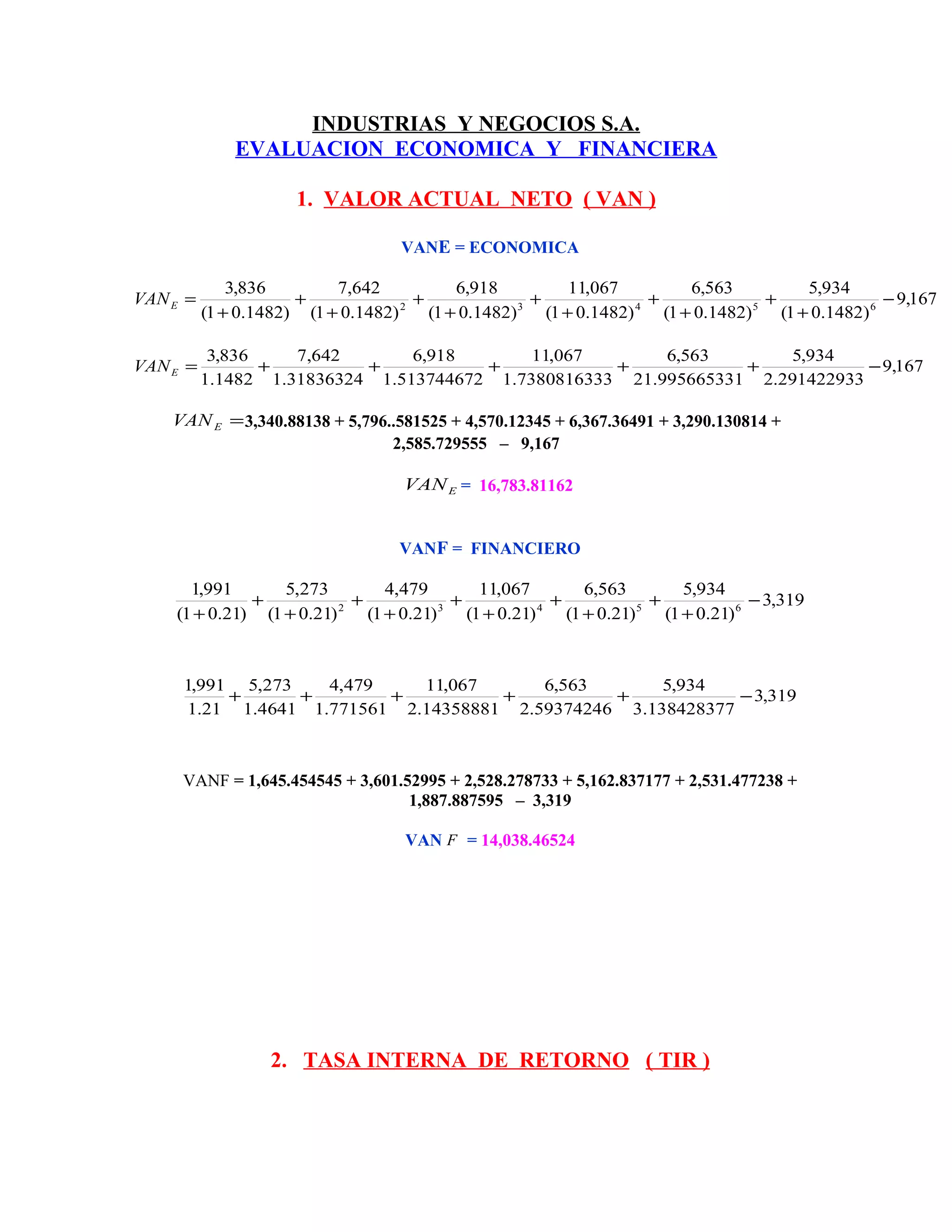
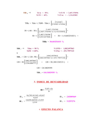
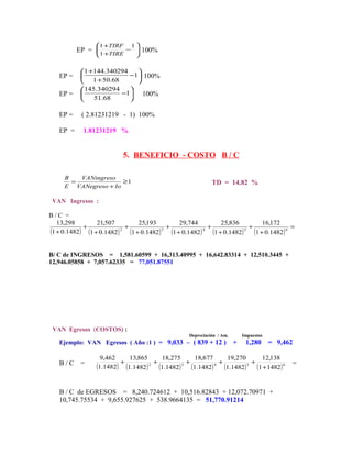
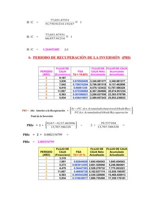
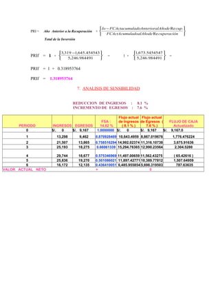
This document provides an economic and financial evaluation of Industrias y Negocios S.A. It includes calculations and analyses of: 1. Net present value (NPV) for both economic and financial scenarios. The economic NPV is $16,783.81 and financial NPV is $14,038.47. 2. Internal rate of return (IRR) for both scenarios. The economic IRR is 50.68% and financial IRR is 144.34%. 3. Payback period, which is 2 years for the economic analysis and 1.32 years for the financial.

1. INDUSTRIAS Y NEGOCIOS S.A.
EVALUACION ECONOMICA Y FINANCIERA
1. VALOR ACTUAL NETO ( VAN )
VANE = ECONOMICA
3,836 7,642 6,918 11,067 6,563 5,934
VAN E = + + + + + − 9,167
(1 + 0.1482) (1 + 0.1482) 2
(1 + 0.1482) 3
(1 + 0.1482) 4
(1 + 0.1482) 5
(1 + 0.1482) 6
3,836 7,642 6,918 11,067 6,563 5,934
VAN E = + + + + + − 9,167
1.1482 1.31836324 1.513744672 1.7380816333 21.995665331 2.291422933
VAN E = 3,340.88138 + 5,796..581525 + 4,570.12345 + 6,367.36491 + 3,290.130814 +
2,585.729555 – 9,167
VAN E = 16,783.81162
VANF = FINANCIERO
1,991 5,273 4,479 11,067 6,563 5,934
+ + + + + − 3,319
(1 + 0.21) (1 + 0.21) 2
(1 + 0.21) 3
(1 + 0.21) 4
(1 + 0.21) 5
(1 + 0.21) 6
1,991 5,273 4,479 11,067 6,563 5,934
+ + + + + − 3,319
1.21 1.4641 1.771561 2.14358881 2.59374246 3.138428377
VANF = 1,645.454545 + 3,601.52995 + 2,528.278733 + 5,162.837177 + 2,531.477238 +
1,887.887595 – 3,319
VAN F = 14,038.46524
2. TASA INTERNA DE RETORNO ( TIR )

2. TIR E → Td m = 50% VAN M = 2,407.378596
Td M = 60% VAN m = - 1,116.03883
 VANM  
TIRe = Tdm + ( TdM – Tdm )  VANM +VANm 

 

 2,407.376596 
50 + ( 60 - 50 )   =
 2,407.378596 + − ,116.03883 
 1 
2,407.376596 
50 + 1   = 50 + 1 ( 0.683251033 ) =
 3,523.417426 
TIRe = 50.683251033 %
TIR f → Tdm = 90 % VANM = 1,082.897063
TdM = 120% VANm = - 251.7997143
9
 1082.897063 
TIR f = 120 + ( 120 - 90 )   =
1082.897063 + −251.7997143
 

1082.897063 
120 + 30  = 120 + 30 ( 0811343131 ) =
1334.696777 

120 + 24.34029395
TIR f = 144.34029395 %
3. INDICE DE RENTABILIDAD
VAN + Io
IR =
Io
16,783.81162 +9,167
IR E = 9,167
IR E = 2.83089469
14,038.46524 + 3,319
IR f = IR f = 5.2297274
3,319
4. EFECTO PALANCA

3. 1 +TIRF 1
EP = 1 +TIRE −  100%
 
 
 1 +144.340294 
EP =  −1 100%
 1 + 50.68 
 145.340294 
EP =  −1 100%
 51.68 
EP = ( 2.81231219 - 1) 100%
EP = 1.81231219 %
5. BENEFICIO - COSTO B / C
B VANingreso
= ≥1 TD = 14.82 %
E VANegreso + Io
VAN Ingresos :
B/C =
13,298 21,507 25,193 29,744 25,836 16,172
+ + + + + =
(1 + 0.1482) (1 + 0.1482) (1 + 0.1482) (1 + 0.1482 ) (1 + 0.1482) (1 + 0.1482) 6
2 3 4 5
B/ C de INGRESOS = 1,581.60599 + 16,313.40995 + 16,642.83314 + 12,510.3445 +
12,946.05858 + 7,057.62335 = 77,051.87551
VAN Egresos (COSTOS) :
Depreciación / Am. Impuestos
Ejemplo: VAN Egresos ( Año :1 ) = 9,033 – ( 839 + 12 ) + 1,280 = 9,462
9,462 13,865 18,275 18,677 19,270 12,138
B/C = + + + + + =
(1.1482) (1.1482 ) (1.1482) (1.1482) (1.1482) (1 + 1482 ) 6
2 3 4 5
B / C de EGRESOS = 8,240.724612 + 10,516.82843 + 12,072.70971 +
10,745.75534 + 9,655.927625 + 538.9664135 = 51,770.91214

4. 77,051.87551
B/C = ≥ 1
51,770.91214 +9,167
77,051.87551
B/C = ≥ 1
60,937.91214
B/C = 1.264432482 ≥1
6. PERIODO DE RECUPERACIÓN DE LA INVERSIÓN (PRI)
FLUJO DE FLUJO DE FLUJO DE CAJA
PERIODO CAJA FSA CAJA Neto Acumulado
(AÑO) (Económico) Td = 14.82% Actualizado Actualizado
0 9,167
1 3,836 0.870928409 3,340.881377 3,340.881377
2 7,642 0.758516294 5,796.581519 9,137.462896
3 6,918 0.66061339 4,570.123432 13,707.586328
4 11,067 0.575346969 6,367.364906 20,074.951234
5 6,563 0.501086021 3,288.627556 23,363.578790
6 5,934 0.436410051 2,589.657243 25,953.236033
Io − FC . Act. AcumuladoAnterioralAñode Re c. 
PRI = Año Anterior a la Recuperación +  
 FCAct. AcumuladoalAñode Re cuperacón 
Total de la Inversión
9,167 −9,137.462896  29.537104
PRIe = 2 +   = 2 + 13,707.586328 =
 13,707.586328 
PRIe = 2 + 0.0002154799 =
PRIe = 2.002154799
FLUJO DE FLUJO DE FLUJO DE CAJA
PERIODO CAJA FSA CAJA Neto Acumulado
(AÑO) (Financiero) Td = 21 % Actualizado Actualizado
0 3,319
1 1,991 0.82644628 1,645.454543 1,645.454543
2 5,273 0.683013455 3,601.529948 5,246.984491
3 4,479 0.56447393 2,528.278732 7,775.263223
4 11,067 0.46650738 5,162.837174 12,938.100397
5 6,563 0.385543289 2,530.320606 15,468.420913
6 5,934 0.318630817 1,890.755268 17,359.176181

5.  Io − FCActacumuladoAnterioralAñode Re cup. 
PRI = Año Anterior a la Recuperación +  
 FCActAcumuladoalAñode Re cuperación 
Total de la Inversión
3,319 −1,645.454543  1,673.5454547 
PRIf = 1 +   = 1 +   =
 5,246.984491   5,246.984491 
PRIf = 1 + 0.318953764
PRIf = 1.318953764
7. ANALISIS DE SENSIBILIDAD
REDUCCION DE INGRESOS : 8.1 %
INCREMENTO DE EGRESOS : 7.6 %
Flujo actual Flujo actual
FSA : de Ingresos de Egresos ( FLUJO DE CAJA
PERIODO INGRESOS EGRESOS 14.82 % ( 8.1 % ) 7.6 % ) Actualizado
0 $/. 0 $/. 9,167 1.0000000 $/. 0 $/. 9,167 $/. 9,167.0
1 13,298 9,462 0.870928409 10,643.4959 8,867.019676 1,776.476224
2 21,507 13,865 0.758516294 14,992.02374 11,316.10738 3,675.91636
3 25,193 18,275 0.66061339 15,294.76365 12,990.23564 2,304.5280
4 29,744 18,677 0.575346969 11,497.00659 11,562.43275 ( 65.42616 )
5 25,836 19,270 0.501086021 11,897.42771 10,389.77812 1,507.64959
6 16,172 12,135 0.436410051 6,485.955854 5,698.319503 787.63635
VALOR ACTUAL NETO = 0