Wave Mechanics Project

Wave Mechanics Project
Anna Ware
Kayley Treichel
Quentin Henderson
Hunter Myres
April 29th, 2015
Texas A&M University at Galveston
Ocean Engineering Department
Instructor: Dr. Masoud Hayatdavoodi

ii
Abstract
This report presents the theoretical and experimental analysis of a storm wave recorded
by a pressure sensor. The application of linear wave theory, Stokes second-order wave theory,
stream function wave theory and cnoidal wave theory are used to determine and compare the
wave parameters. Experimental analysis is performed using a model scale wave produced by a
wave flume. The effect of adding cylinders in the wave’s path is examined as well as the forces
on these cylinders. Lastly, the placement of a wind turbine behind a breakwater is determined in
order to minimize the wave height on the turbine.

Table of Contents
Abstract............................................................................................................................................ii
1.0 Introduction ............................................................................................................................... 1
2.0 Definition of variables and equations ....................................................................................... 1
2.1 Variables ............................................................................................................................... 1
2.2 Equations .............................................................................................................................. 2
3.0 Theoretical analysis .................................................................................................................. 2
3.1 Estimation of Wave Parameters........................................................................................... 3
3.1.1 Linear Wave Theory ....................................................................................................... 3
3.1.2 Stokes Second-Order Wave Theory.............................................................................. 4
3.1.3 Stream Function Wave Theory ...................................................................................... 5
3.1.4 Comparison of the Wave Profile for each Wave Theory ............................................... 5
3.1.5 Comparison of the hydrodynamic pressure on the seafloor for each wave theory....... 6
3.1.6 Comparison of the hydrodynamic pressure on the water column for each wave theory
................................................................................................................................................. 6
3.1.7 Comparison of the horizontal water particle velocity on the water column for each
wave theory.............................................................................................................................. 8
3.1.8 Applicability of wave theories ......................................................................................... 9
3.2 Estimation of Wave Parameters (extra credit)...................................................................... 9
3.2.1 Linear Wave Theory ....................................................................................................... 9
3.2.2 Stokes Second-Order Wave Theory............................................................................ 11
3.2.3 Stream Function Wave Theory .................................................................................... 11
3.2.4 Cnoidal Wave Theory................................................................................................... 11
3.2.5 Comparison of the wave profile for each wave theory................................................. 11
3.2.6 Comparison of the Hydrodynamic Pressure on the Seafloor for each Wave Theory . 12
3.2.7 Comparison of the Hydrodynamic Pressure on the Water Column for each Wave
Theory.................................................................................................................................... 13
3.2.8 Comparison of the Horizontal Water Particle Velocity on the Water Column for each
Wave Theory.......................................................................................................................... 14
3.2.9 Applicability of Wave Theories ..................................................................................... 16
4.0 Experimental Analysis ............................................................................................................ 16
4.1 Comparison of Laboratory Measurements and Theoretical Results of Surface Elevation 16
4.2 Comparison of laboratory measurements and theoretical results of total pressure .......... 17
4.3 Wave Power........................................................................................................................ 19

4.4 Comparisons of Surface Elevations and Total Seafloor Pressures with the Addition of One
or Two Vertical Cylinders .......................................................................................................... 19
5.0 Design..................................................................................................................................... 21
5.1 Force on a Prototype Scale Cylinder near Pressure Sensor............................................. 21
5.2 Force on Downwave Cylinder near Pressure Sensor........................................................ 22
5.3 Placement of a Floating Wind Turbine ............................................................................... 23
6.0 Conclusion .............................................................................................................................. 26
7.0 References.............................................................................................................................. 27
8.0 Appendix ................................................................................................................................. 28

1
1.0 Introduction
During a storm event, a pressure sensor on the seafloor recorded a pressure fluctuation
ranging from 106.5 kPa to 104.5 kPa with a period of 4 seconds. Based on the given wave
pressure differential and period, linear, Stokes second-order and stream function wave theories
were used to estimate the water depth, wave height, wave length, and celerity of the waves
generated by the storm. For each theory, these estimates were used to plot the wave profiles and
hydrodynamic pressure on the seafloor. Next, these values were used to generate plots of the
distributions of hydrodynamic pressure and horizontal water particle velocity under the crest and
trough of the wave. The comparisons of the wave property plots were used to determine the
applicability of the four wave theories.
Experiments were then conducted by simulating the linear wave solution to the problem in
a wave flume. The wave parameters were scaled using Froude scaling laws in order for the
model wave to relate to the collected prototype storm wave. The data from this experiment was
compared with the theoretical data. The wave power for the storm wave was found using the
measurement of surface elevation from the experiment.
The effect of a vertical cylinder, or offshore platform leg, on a wave was then determined
using the wave flume. One vertical cylinder was placed in the wave flume 10 cm upwave from
the first wave gauge. The diffracted wave profile and pressure on the seafloor was compared
with the non-diffracted wave profile from the previous experiment. A second cylinder was
introduced 10 cm from the initial cylinder, and this wave profile was also compared to the non-
diffracted wave profile.
Using the data from the experiment with the cylinders, Morison’s equation was used to
determine the total wave force on the prototype scale of the vertical cylinder. The same equation
was used to determine the wave forces on a cylinder downwave of the initial cylinder. Using the
initial linear wave theory wave characteristics, the placement of a floating wind turbine was
optimized so that the wave height at the point of placement was the smallest it could be.
2.0 Definition of variables and equations
Variables and equations that will be used in the following chapters are defined in this
chapter. The equations are numbered for reference in later chapters.
2.1 Variables
1. 𝜌 = 𝐷𝑒𝑛𝑠𝑖𝑡𝑦 𝑜𝑓 𝑤𝑎𝑡𝑒𝑟,1025
𝑘𝑔
𝑚3
( 𝑠𝑒𝑎𝑤𝑎𝑡𝑒𝑟),
1000𝑘𝑔
𝑚3 (𝑓𝑟𝑒𝑠ℎ 𝑤𝑎𝑡𝑒𝑟)
2. 𝑔 = 𝐴𝑐𝑐𝑒𝑙𝑒𝑟𝑎𝑡𝑖𝑜𝑛 𝑑𝑢𝑒 𝑡𝑜 𝑔𝑟𝑎𝑣𝑖𝑡𝑦, 9.81
𝑚
𝑠2
3. 𝑥2 = 𝐷𝑖𝑠𝑡𝑎𝑛𝑐𝑒 𝑓𝑟𝑜𝑚 𝑡ℎ𝑒 𝑠𝑡𝑖𝑙𝑙 𝑤𝑎𝑡𝑒𝑟 𝑙𝑒𝑣𝑒𝑙

2
4. 𝑇 = 𝑃𝑒𝑟𝑖𝑜𝑑 (𝑠)
5. 𝑘 = 𝑊𝑎𝑣𝑒 𝑛𝑢𝑚𝑏𝑒𝑟 (𝑚−1
)
6. 𝑥1 = 𝐷𝑖𝑠𝑡𝑎𝑛𝑐𝑒 𝑓𝑟𝑜𝑚 𝑜𝑟𝑖𝑔𝑖𝑛 𝑎𝑙𝑜𝑛𝑔 𝑡ℎ𝑒 𝑠𝑡𝑖𝑙𝑙 𝑤𝑎𝑡𝑒𝑟 𝑙𝑖𝑛𝑒
7. 𝑡 = 𝑇𝑖𝑚𝑒 𝑖𝑛 𝑠𝑒𝑐𝑜𝑛𝑑𝑠
8. 𝐷 = 𝑑𝑖𝑎𝑚𝑒𝑡𝑒𝑟 𝑜𝑓 𝑟𝑒𝑑 𝑐𝑦𝑙𝑖𝑛𝑑𝑒𝑟 𝑖𝑛 𝑤𝑎𝑣𝑒 𝑡𝑎𝑛𝑘 𝑒𝑥𝑝𝑒𝑟𝑖𝑚𝑒𝑛𝑡
2.2 Equations
All Wave Theory
Hydrostatic pressure: 𝑃 = −𝜌𝑔𝑥2 (1)
Wave frequency: 𝜔 =
2𝜋
𝑇
(2)
Wave length: 𝜆 =
2𝜋
𝑘
(3)
Dispersion relation: 𝜔2
= 𝑔𝑘𝑡𝑎𝑛ℎ(𝑘ℎ) (4)
Celerity: 𝑐 =
𝜆
𝑇
(5)
Morison’s Equation: 𝑑𝐹 = 𝑑𝐹𝐼 + 𝑑𝐹𝐷 = 𝐶 𝑚 𝜌𝜋(
𝐷
2
)2 𝑑𝑈1
𝑑𝑡
+
𝐷𝜌𝐶 𝑑 𝑈1| 𝑈1|
2
(6)
Linear Wave Theory
Pressure field equation: 𝑃 =
𝜌𝑔𝐻
2
(
cosh(𝑘( 𝑥2+ℎ))
cosh(𝑘ℎ)
)cos( 𝑘𝑥1 − 𝜔𝑡) − 𝜌𝑔𝑥2 (7)
Hydrodynamic pressure: 𝑃 =
𝜌𝑔𝐻
2
(
cosh(𝑘ℎ)
)cos( 𝑘𝑥1 − 𝜔𝑡) (8)
Surface elevation: 𝜂 =
𝐻
2
cos(𝑘𝑥1 − 𝜔𝑡) (9)
Horizontal particle velocity: 𝑈1 =
𝐻
2
𝑔𝑇
𝜆
cosh(𝑘ℎ)
cos(𝑘𝑥1 − 𝜔𝑡) (10)
Horizontal water particle acceleration:
𝑑𝑈1
𝑑𝑡
=
𝐻𝑔𝑇
𝜆
cosh(𝑘ℎ)
sin(𝑘𝑥1 − 𝜔𝑡) (11)
Wave Power: 𝑃0 =
𝜌𝑔𝐻2
𝜆
16𝑇
(1 +
2𝑘ℎ
sinh(2𝑘ℎ)
) (12)
Stokes Wave Theory
Pressure field equation: 𝑃 =
𝜌𝑔𝐻
2
(
cosh(𝑘(𝑥2+ℎ) )
cosh(𝑘ℎ)
)cos( 𝑘𝑥1 − 𝜔𝑡) − 𝜌𝑔𝑥2
+
3𝜌𝑔𝐻
4
( 𝜋𝐻
𝜆
) 1
sinh (2𝑘ℎ)
[
cosh(2𝑘 (𝑥2+ℎ) )
sinh(𝑘ℎ) 2
−
1
3
] cos(2(𝑘𝑥1 − 𝜔𝑡)) −
𝜌𝑔𝐻
4
( 𝜋𝐻
𝜆
) 1
sinh (2𝑘ℎ)
[cosh(2𝑘( 𝑥2 + ℎ)) − 1] (13)
Surface elevation: 𝜂 =
𝐻
2
cos( 𝑘𝑥1 − 𝜔𝑡) +
𝐻
2
𝜋𝐻
𝜆
sinh(𝑘ℎ)3 cos(2( 𝑘𝑥1 − 𝜔𝑡)) (14)
Horizontal particle velocity: 𝑈1 =
𝜋𝐻
𝑇
sinh(𝑘ℎ)
cos( 𝑘𝑥1 − 𝜔𝑡) +
3
4
𝜋𝐻
𝑇
𝜋𝐻
𝐿
cosh(2𝑘( 𝑥2+ℎ))
sinh(𝑘ℎ)4 sin(2( 𝑘𝑥1 − 𝜔𝑡)) (15)
3.0 Theoretical analysis
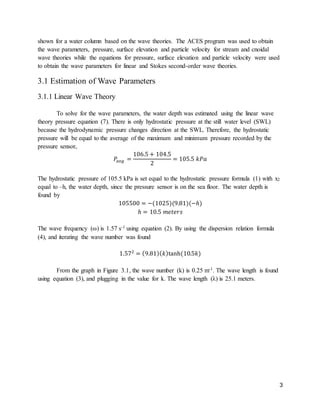
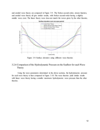
The wave parameters for the storm wave were determined using linear wave theory,
Stokes second-order wave theory and stream function wave theory (cnoidal wave theory was
also used for section 3.2). The wave profile and hydrodynamic seafloor pressure were plotted
over a wave period and compared with each of the wave theories. The distributions of the
hydrodynamic pressure and horizontal water particles velocity under the crest and trough were

3
shown for a water column based on the wave theories. The ACES program was used to obtain
the wave parameters, pressure, surface elevation and particle velocity for stream and cnoidal
wave theories while the equations for pressure, surface elevation and particle velocity were used
to obtain the wave parameters for linear and Stokes second-order wave theories.
3.1 Estimation of Wave Parameters
3.1.1 Linear Wave Theory
To solve for the wave parameters, the water depth was estimated using the linear wave
theory pressure equation (7). There is only hydrostatic pressure at the still water level (SWL)
because the hydrodynamic pressure changes direction at the SWL. Therefore, the hydrostatic
pressure will be equal to the average of the maximum and minimum pressure recorded by the
pressure sensor,
𝑃𝑎𝑣𝑔 =
106.5 + 104.5
2
= 105.5 𝑘𝑃𝑎
The hydrostatic pressure of 105.5 kPa is set equal to the hydrostatic pressure formula (1) with x2
equal to –h, the water depth, since the pressure sensor is on the sea floor. The water depth is
found by
105500 = −(1025)(9.81)(−ℎ)
ℎ = 10.5 𝑚𝑒𝑡𝑒𝑟𝑠
The wave frequency (ω) is 1.57 s-1 using equation (2). By using the dispersion relation formula
(4), and iterating the wave number was found
1.572
= (9.81)( 𝑘)tanh(10.5𝑘)
From the graph in Figure 3.1, the wave number (k) is 0.25 m-1. The wave length is found
using equation (3), and plugging in the value for k. The wave length (λ) is 25.1 meters.

4
Figure 3.1: Solution of dispersion relation to find wave number
The max pressure occurs when cos( 𝑘𝑥1 − 𝜔𝑡) = 1 and the minimum pressure occurs
when cos( 𝑘𝑥1 − 𝜔𝑡) = −1. Since x2 is equal to –h, cosh(𝑘( 𝑥2 + ℎ)) = 1 for both minimum
and maximum pressures. By subtracting the minimum pressure equation from the maximum
pressure equation, the wave height is found using
𝐻 =
cosh((0.25)(10.5))(106.5 − 104.5)
(1.025)(9.81)
= 1.38𝑚
By using equation (5) the celerity is
𝑐 =
25.1
4
= 6.275 𝑚/𝑠
Linear theory was utilized to estimate the water depth, wave height, wave length, and
celerity as 10.5 meters, 1.38 meters, 25.1 meters, and 6.275 m/s, respectively.
3.1.2 Stokes Second-OrderWave Theory
The pressure equation for Stokes second-order wave theory (Equation 13) was used to
determine the wave height, water depth, wave length and celerity of the storm wave. Unlike the
linear solution, the hydrostatic term cannot be isolated because there is an additional term that
arises when subtracting Pmax by Pmin. A MATLAB code was created to in order test possible
values of water depth, wave height and wave number in order to get pressures that were close to
the recorded maximum and minimum. Using the code, the wave height was taken as 1.39 meters,

5
the water depth was 10.49 meters and the wave number was 0.251 m-1. This gives a wave length
of 25.03 meters and celerity of 6.26 m/s.
3.1.3 Stream Function Wave Theory
ACES was utilized to estimate the water depth, wave height, wave length, and celerity for
the stream function wave theory. The estimated values for wave height and water depth using
linear wave theory of 10.5 meters, and 1.38 meters respectively and a period of 4 seconds were
input into the program. The max pressure given by ACES is 106.54 kPa, and the minimum
pressure is 104.54 kPa. These pressures have a percent error much less than 1% with the given
pressure values. The wave height, wave number, celerity, and wavelength given by the program
are 1.38 meters, 0.249 m-1, 6.30 m/s, and 25.19 meters, respectively.
3.1.4 Comparison of the Wave Profile for each Wave Theory
Using the wave parameters determined in Sections 3.1.1-3.1.3, the surface elevation of
the wave for linear wave theory, Stokes second-order wave theory and stream function wave
theory are compared in Figure 3.2. The Stokes second-order and stream function wave theory
have slightly higher crests and troughs than the linear theory wave.
Figure 3.2: Surface elevation using different wave theories

6
3.1.5 Comparison of the hydrodynamic pressure on the seafloor for each wave
theory
Using the water parameters determined in the above sections, the hydrodynamic pressure
for each wave theory is then compared in Figure 3.3. The wave theories all yield approximately
the same results.
Figure 3.3: Hydrodynamic pressure using different wave theories
3.1.6 Comparison of the hydrodynamic pressure on the water column for each
wave theory
The hydrodynamic pressure under the crest, down the water column, is compared for the
linear, Stokes second-order and stream function wave theories in Figure 3.4. The graph shows
good agreement between the three wave theories with the linear theory having a larger
hydrodynamic pressure.

7
Figure 3.4: Hydrodynamic pressure under wave crest
The hydrodynamic pressure under the trough is compared for the three wave theories in
Figure 3.5. The stream function line does not continue to the surface of the water because there is
no water above a certain height, due to the wave height. The Stokes second-order wave theory
gives the largest hydrodynamic pressure under the trough.
Figure 3.5: Hydrodynamic pressure under wave trough

8
3.1.7 Comparison of the horizontal water particle velocity on the water column for
each wave theory
The horizontal water particle velocity under the crest, down the water column, was
compared for linear, Stokes second-order and stream function wave theories. The results are
shown in Figure 3.6, where all theories give similar results. The stream function gives slightly
smaller velocities down the water column.
Figure 3.6: Horizontal water particle velocity under wave crest
The horizontal water particle velocity under the trough is compared for the three wave
theories in Figure 3.7. The stream function line, which gives the largest particle velocity, does
not continue to the water surface because there is no water, due to the wave height.

9
Figure 3.7: Horizontal water particle velocity under wave trough
3.1.8 Applicability of wave theories
From the preceding sections, the applicability of the each wave theory to the storm wave
can be analyzed. Linear, Stokes-second order and stream function wave theory provided similar
answers for the surface elevation, hydrodynamic pressure and horizontal water particle velocity.
Therefore, the three wave theories can be applied to describe the storm wave with minimal error.
3.2 Estimation of Wave Parameters (extra credit)
This section is similar to Section 3.1 but the maximum pressure, minimum pressure and
wave period are changed are changed to 124.4 kPa, 86.7 kPa and 10 seconds. The procedure and
methodology for this section is the same as the preceding section.
3.2.1 Linear Wave Theory
To solve for the wave parameters, the water depth was estimated using the linear wave
theory pressure equation (7). There is only hydrostatic pressure at the still water level (SWL)
because the hydrodynamic pressure changes direction at the SWL. Therefore, the hydrostatic
pressure will be equal to the average of the maximum and minimum pressure recorded by the
pressure sensor,
𝑃𝑎𝑣𝑔 =
124.4 + 86.7
2
= 105.55 𝑘𝑃𝑎

10
The hydrostatic pressure of 105.55 kPa is set equal to the hydrostatic pressure formula (1) with
x2 equal to –h, the water depth since the pressure sensor is on the sea floor. The water depth is
found by
105550 = −(1025)(9.81)(−ℎ)
ℎ = 10.5 𝑚𝑒𝑡𝑒𝑟𝑠
The wave frequency (ω) is 0.628 s-1 using equation (2). By using the dispersion relation formula
(4) and iterating, the wave number was found
0.6282
= (9.81)( 𝑘)tanh(10.5𝑘)
From the graph in Figure 3.8, the wave number (k) is 0.066 m-1. The wave length is
found using equation (3), and plugging in the value for k. The wave length (λ) is 95.2 meters.
The max pressure occurs when cos( 𝑘𝑥1 − 𝜔𝑡) = 1 and the minimum pressure occurs at
cos( 𝑘𝑥1 − 𝜔𝑡) = −1. Since x2 is equal to –h, cosh(𝑘( 𝑥2 + ℎ)) = 1 for both minimum and
maximum pressures. By subtracting the minimum pressure equation from the maximum pressure
equation, the wave height was found using
𝐻 =
cosh((0.066)(10.5))(124.4 − 86.7)
(1.025)(9.81)
= 4.69𝑚
By using equation (5) the celerity is
𝑐 =
95.2
10
= 9.52 𝑚/𝑠

11
Linear theory was utilized to determine the water depth, wave height, wave length, and
celerity as 10.5 meters, 4.69 meters, 95.2 meters, and 9.52 m/s, respectively.
3.2.2 Stokes Second-OrderWave Theory
The pressure equation for Stokes second-order wave theory (Equation 13) was used to
determine the wave height, water depth, wave length and celerity of the storm wave. Unlike the
linear solution, the hydrostatic term cannot be isolated because there is an additional term that
arises when subtracting Pmax by Pmin. A MATLAB code was created in order to test possible
values of water depth, wave height and wave number in order to get pressures that were close to
the recorded maximum and minimum. Using the code, the wave height was taken as 4.72 meters,
the water depth was 10.08 meters and the wave number was 0.07 m-1. This gives a wave length
of 89.76 meters and celerity of 8.98 m/s.
3.2.3 Stream Function Wave Theory
The ACES program was utilized to estimate the water depth, wave height, wave length,
and celerity for the Stream function wave theory. The values for wave height and water depth
using linear wave theory, 10.5 meters and 4.69 meters respectively, and a period of 10 seconds
were input into the program. The wave height and water depth were adjusted until a maximum
pressure of 125.41 kPa, and a minimum pressure of 86.77 kPa were determined. The pressures
given by ACES are within a 1% error of the given pressures. The water depth, wave height,
wavelength, and celerity given by the program are 10 meters, 6.5 meters, 100.89 meters, and
10.89 m/s respectively.
3.2.4 Cnoidal Wave Theory
ACES was also used to estimate the water depth, wave height, wave length, and celerity
for the second order cnoidal wave theory. The water depth of 10.5 meters and wave height of
4.69 meters from linear wave theory, and a period of 10 seconds were input into the program.
These values were adjusted until the maximum pressure of 124.96 kPa and a minimum pressure
of 86.01 kPa were determined. The pressures are within 1% error of the given pressures. The
water depth, wave height, wavelength, and celerity given by the program are 10.11 meters, 6.5
meters, 97.92 meters, and 9.79 m/s, respectively.
3.2.5 Comparison of the wave profile for each wave theory
Using the wave parameters determined in Sections 3.2.1-3.2.4, the surface elevation of
the wave for linear wave theory, Stokes second-order wave theory stream function wave theory

12
and cnoidal wave theory are compared in Figure 3.9. The Stokes second-order, stream function,
and cnoidal wave theory all give similar results, with Stokes second-order having a slightly
smaller wave crest. The linear theory wave does not match the waves given by the other theories.
Figure 3.9: Surface elevation using different wave theories
3.2.6 Comparison of the Hydrodynamic Pressure on the Seafloor for each Wave
Theory
Using the wave parameters determined in the above sections, the hydrodynamic pressure
for each wave theory is then compared in Figure 3.10. The wave theories yield similar results
with linear wave theory having a smaller maximum hydrodynamic wave pressure than the other
theories.

13
Figure 3.10: Hydrodynamic pressure using different wave theories
3.2.7 Comparison of the Hydrodynamic Pressure on the Water Column for each
Wave Theory
The hydrodynamic pressure under the crest, down the water column, is compared for the
linear, Stokes second-order stream function, and cnoidal wave theories in Figure 3.11. The wave
theories result in different water depths, which explains the different ending points at the
seafloor. Cnoidal theory has a significantly larger hydrodynamic pressure near the still water line
than the other theories.
Figure 3.11: Hydrodynamic pressure under wave crest

14
The hydrodynamic pressure under the trough is compared for the four wave theories in
Figure 3.12. The stream function and cnoidal theory do not continue to the surface of the water
because there is no water above a certain height, due to the wave height. The linear theory gives
a larger hydrodynamic pressure than the other wave theories.
Figure 3.12: Hydrodynamic pressure under wave trough
3.2.8 Comparison of the Horizontal Water Particle Velocity on the Water Column
for each Wave Theory
The horizontal water particle velocity under the crest, down the water column, is
compared for linear, Stokes second-order, stream function and cnoidal wave theories. The results
are shown in Figure 3.13, where the Stokes second-order wave theory gives the largest horizontal
particle velocity.

15
Figure 3.13: Horizontal water particle velocity under wave crest
The horizontal water particle velocity under the trough is compared for the four wave
theories in Figure 3.14. The stream function and cnoidal lines do not continue to the water
surface because there is no water, due to the wave height. The Stokes second-order line appears
to increase slightly as the particle moves down the water column. This behavior was not
exhibited in the other wave theories and is due to the nonlinear term in the Stokes second-order
equation for horizontal water particle velocity.
Figure 3.14: Horizontal water particle velocity under wave trough

16
3.2.9 Applicability of Wave Theories
From the preceding sections, the applicability of the each wave theory to the storm wave
can be analyzed. Linear, Stokes-second order, stream function and cnoidal wave theory provide
different solutions to the same wave. The stream function and cnoidal wave theories yield similar
results for the surface elevation comparison. The hydrodynamic pressure and horizontal particle
velocity are different for the four linear theories.
4.0 Experimental Analysis
Froude similarity and the water depth ratio were used to transfer between model and
prototype scales. The wave period for the model (wave flume) was found using Froude similarity
along with the water depth ratio to scale down the wave length. A non-dimensional pressure
relation was used to scale between the model and prototype pressures. For more details
concerning the scaling factors refer to Appendix 1.
4.1 Comparison of Laboratory Measurements and Theoretical Results of
Surface Elevation
Figure 4.1 shows a comparison of the prototype scale surface elevation for experimental
data and results of linear, Stokes second-order, and stream function wave theories. The
experimental data is in good agreement with the theoretical results. The experimental wave
height is slightly smaller than all of the wave theories and shows a plateaued wave crest. The
experimental and stream function also show a slight change in wave period.
Figure 4.1: Experimental surface elevation compared with results of different wave theories

17
4.2 Comparison of laboratory measurements and theoretical results of
total pressure
Total pressure on the seafloor at the prototype scale for the experimental wave is
compared to the theoretical seafloor pressures in Figure 4.2. The experimental pressure is noisy,
but does follow a sinusoidal form close to the three wave theories shown.
Figure 4.2: Total experimental pressure at the seafloor compared to three wave theories
Figure 4.3 shows the total pressure at pressure sensor 1 for the experimental wave data
and wave theories. The depth of pressure sensor 1 was scaled to prototype length in order to
determine the theoretical pressures at an equivalent location. The experimental pressure is also
shown at prototype scale. The experimental pressure follows the sinusoidal form of the
theoretical pressures well. This can also be said for Figure 4.4, which compares the total
pressures at the prototype location corresponding to pressure sensor 2. For scaling details see
Appendix 1.

18
Figure 4.3: Total experimental pressure compared to the three wave theories at sensor 1
Figure 4.4: Total experimental pressure at sensor 2 compared to three wave theories

19
4.3 Wave Power
Using the laboratory measurements for the surface elevation (shown in Figure 4.1), the
wave power of the prototype wave was determined. The prototype wave period and wave height
given by the laboratory measurements is 3.8 seconds and 1.18 meters. The slight difference in
wave period between the experimental and theoretical is due to rounding errors when inputting
data into the wave flume program. The wave number, 0.280 m-1, was determined using Figure
4.5 and the wave length is 22.44 meters. Using Equation 12, the wave power per wavelength is
5337.3 W. This represents the power per unit width for one wavelength.
4.4 Comparisons of Surface Elevations and Total Seafloor Pressures
with the Addition of One or Two Vertical Cylinders
In Figure 4.6, the surface elevations for the cases of one vertical cylinder and two vertical
cylinders are compared with the non-diffracted experimental surface elevation. Given material
limitations, the second cylinder is a triangular prism comprised of smaller cylinders. The troughs
of the case with one vertical cylinder present appear non-linear. There is also an increase in wave
height of approximately 15% when compared with the non-diffracted wave profile. The case
with two vertical cylinders shows a profile that closely mimics the non-diffracted case. The non-
linearity caused by one cylinder is no longer present and the wave height is reduced back to the
non-diffracted case. The increase in wave height with one cylinder is possibly due to diffraction
of the wave around the cylinder and reflection of the waves against the walls of the wave flume.
The reduction of wave height when the second cylinder is added could be because of the actual

20
shape of the cylinder object used. The second object was more of a triangular prism than an
actual cylinder. With an edge of the prism orthogonal to the wave crests, some of the wave
energy could have been reflected from two of the prism faces. A top view diagram of the wave
flume used is shown in Figure 4.7 with the two cylinder setup.
Figure 4.6: Experimental surface elevations for one, two and no cylinders
Figure 4.7: Top view of wave flume
Figure 4.8 shows a comparison of the seafloor pressure for the three above mentioned
scenarios. The seafloor pressures do follow a general sinusoidal form, but no strong conclusions
can be made from the data.

21
Figure 4.8: Total pressure at the seafloor for the one, two and no cylinder cases
5.0 Design
5.1 Force on a Prototype Scale Cylinder near Pressure Sensor
A prototype scale of the red cylinder used in the laboratory experiment is located close to
the pressure sensor offshore. The Morison’s equation (Equation 6) was used to calculate and plot
the inertia force, drag force and total force on the vertical cylinder over one wave period. The Cm
and Cd were assumed to be 2 and 1.2, respectively. In the laboratory experiment, the diameter of
the red cylinder was 0.11 meters. The diameter of the prototype cylinder is the scaled up version
of the model cylinder. The scaling factor can be seen in Appendix 1 and gives a prototype
diameter of 4.62 meters.
In order to use Morison’s equation, the wave parameters of the experimental wave found
in Section 4.3 were used. The horizontal water particle velocity and the horizontal water particle
acceleration (Equations 10 and 11) were found at different water depths down the water column.
A MATLAB code was generated in order to evaluate the integral of Morison’s equation over a
wave period. Figure 5.1 shows the drag force, inertia force and total force on the entire
submerged cylinder over one wave period. The drag force oscillates more than the inertia force
while the inertia force is much larger than the drag force on the cylinder.

22
Figure 5.1: Force on prototype cylinder over one wave period
5.2 Force on Downwave Cylinder near Pressure Sensor
In order to estimate the wave loads on the cylinder downwave, the wave height after the
wave hits the first cylinder needed to be determined. Section 4.4 gives the wave height to be
approximately 1.36 meters. This information was used in the MATLAB code generated to find
the force on the entire cylinder. Figure 5.2 shows the force on the downwave cylinder over one
wave period. It is important to note that the force on the downwave cylinder is greater than the
force on the upwave cylinder. This was due to the wave height being greater on the second
cylinder than it was on the first cylinder (see Section 4.4). The wave height was greater due to
reflection of the wave off of the wave tank’s sides. In the real world, there are no wave tank sides
that would reflect the wave’s energy. Therefore, the wave height would be less on the second
cylinder and the force would be less.

23
Figure 5.2: Force on downwave prototype cylinder over one wave period
5.3 Placement of a Floating Wind Turbine
A floating wind turbine needs to be installed close to the shoreline behind a breakwater in
order to harvest wind energy. On the shore side of the breakwater, the water depth is 5 meters.
For the design problem, the bottom contours and shoreline are assumed to be parallel and
straight, with a uniform slope in the upwave region. The incoming waves make a 45ᵒ angle with
the bottom contours. The breakwater is 4λi in length and is located 6λi from the shoreline, where
λi is the wave length of the wave after shoaling and refraction have occurred. The wind turbine
must be placed 3λi from the shore. Figure 5.3 shows the setup of the problem as well as the line
along which the wind turbine can be placed.

24
Figure 5.3: Placement of wind turbine problem
The solution of this problem begins with determining the wave height and wavelength of
the storm wave when it is right at the breakwater. The effects of shoaling and refraction will
change the wave height, wavelength and angle of the incoming wave. The linear solution from
Section 3.1.1 will be used in solving this problem. The wave height is 1.38 meters and the
wavelength is 25.1 meters. The shoaling coefficient, Ks, and refraction coefficient, Kr, are
determined to be 0.95 and 0.9, respectively. The new incoming angle of the wave is 37ᵒ (with
respect to the bottom contours. The new wave height is determined by
𝐻𝑖 = 𝐻𝐾𝑟 𝐾𝑠
and is equal to 1.18 meters. The new wavelength was determined using the dispersion relation
(Equation 4) and graphing to determine the wave number. The results of the graph are shown in
Figure 5.4 and yield a wave number of 0.283 m-1 and a wave length of 22.2 meters. The effects
of shoaling and refraction have been accounted for, now the effects of diffraction must be
determined.

25
Diffraction occurs at the left and right hand side of the breakwater. In order to place the
wind turbine at the location with the smallest wave height, the diffraction due to both sides of the
breakwater must be considered. The diffraction coefficient must be determined and it depends on
the angle the wave makes with the breakwater, the angle to the point of interest, and the ratio of
the distance to the point divided by the wavelength at the breakwater. Figure 5.5 shows a
diagram with the important variables labeled.
Figure 5.5: Diffraction problem
To find the diffraction coefficient at the point of interest, the diffraction coefficient due to
the left side of the breakwater must be added with that of the right side. The incoming wave
angle (37ᵒ and 143ᵒ) is not a round number that appears on the wave diffraction coefficient table,
so bilinear interpolation must be done to determine the Kd for the left and right hand side of the

26
breakwater. A MATLAB code was created to determine the Kd and wave height depending on
the placement location’s distance from the left hand side. From the results of the code, Figure 5.6
is constructed and the optimal placement of wind turbine is directly below the left hand side of
the breakwater. At this point, the wave height is 0.8774 meters.
Figure 5.6: Wave height at distance x from left side of breakwater
6.0 Conclusion
The application of linear wave theory, Stokes second-order wave theory, stream function
wave theory and cnoidal wave theory were used to determine and compare the wave parameters
of the storm waves. Each of the wave theories appeared to accurately represent the storm waves.
Experimental analysis was performed using a model scale wave produced by a wave flume. The
wave parameters obtained through the wave flume were also compared to the theoretical
parameters. Morison’s equation was used to determine the forces on an upwave and downwave
cylinder based on laboratory experiments. The placement of a wind turbine behind a breakwater
was determined in order to minimize the wave height on the turbine.

27
7.0 References
OCEN300 Wave Mechanics class materials

29
Appendix 2: Code used in project

Wave Mechanics Project

More Related Content

Similar to Wave Mechanics Project

Wave Mechanics Project