DAM knowldge

1. 5. Reservoir
Prepared by: Birhanu W. 1

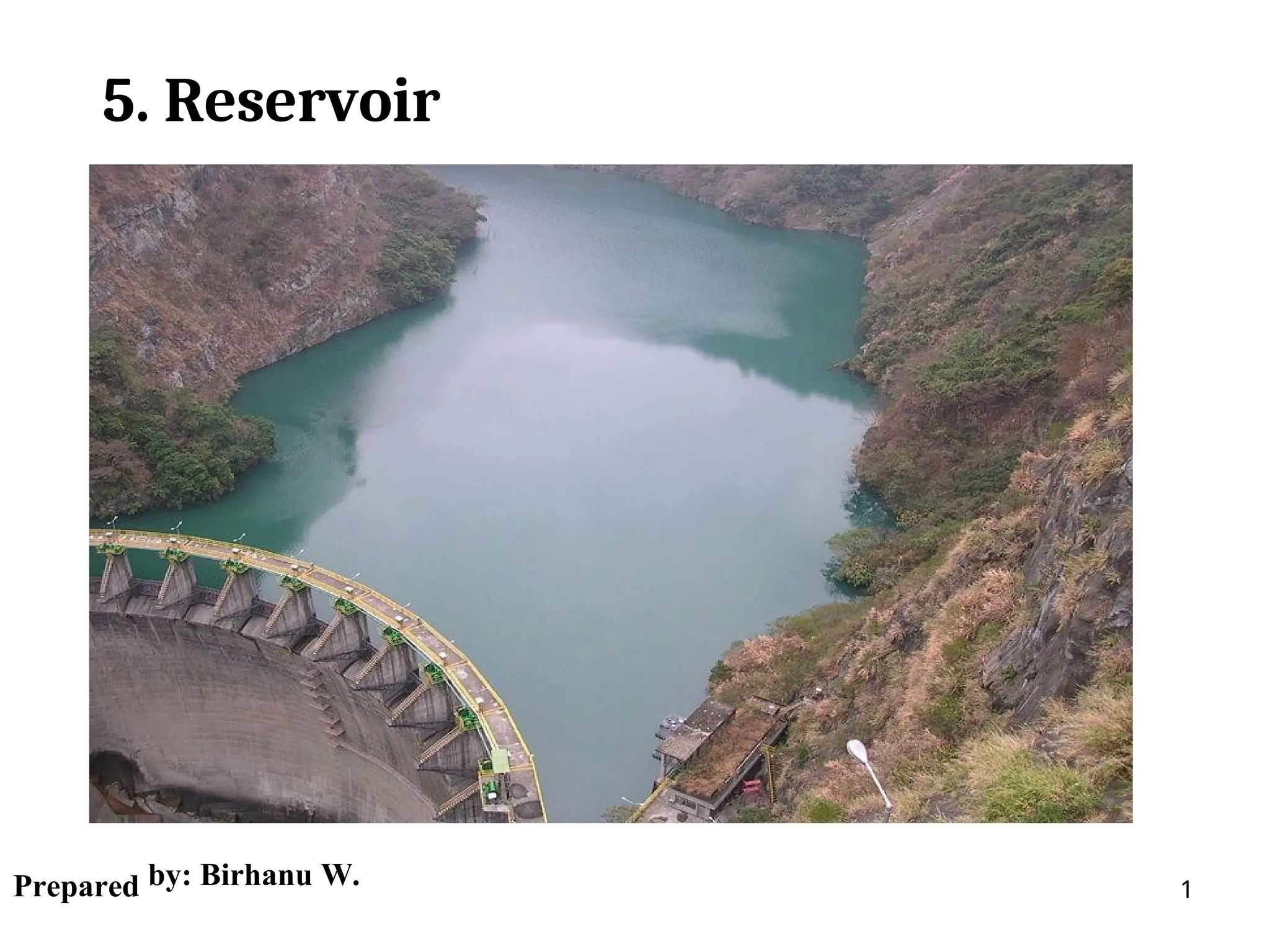
2. Reservoir: During high flows, water flowing in a river has to be stored so
that a uniform supply of water can be assured, for water resources
utilisation like irrigation, water supply, power generation, etc. during
periods of low flows of the river.
Its determination is performed using historical inflow records in the stream
at
the proposed dam site.
 Type of Reservoir
Storage or conservation reservoir
 Can retain excess supplies during period of peak flows and can
release gradually during low flows
Flood control reservoir
 to minimize the flood peaks at the areas to be protected
downstream. Multipurpose reservoir
5.1 Reservoir

3.  designed to protect the downstream areas from floods and to conserve
water
for water supply, irrigation, industrial needs, hydroelectric purposes etc
Distribution reservoir 2
 Is a small storage reservoir constructed within a city water supply system

4. 3
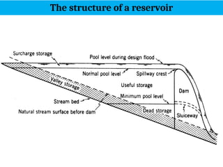
5.1.1 Storage Zone of Reservoir
• Normal pool level: It is the maximum
elevation, to which the reservoir water
surface will rise during normal operating
condition.
• Minimum pool level: The lowest water
surface elevation, which has to be kept under
normal operating condition in a reservoir
• Surcharge storage: This is the storage between
full reservoir level and maximum water level.

5. 4
• Dead storage (low water level): It is the
minimum reservoir level below which, water is
not allowed to be drawn for conservation
purposes.

6. 5
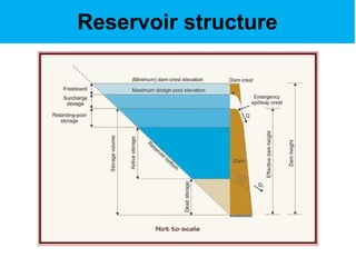
Storage Zone of Reservoir
• Live storage: It is also known as the useful or
conservation storage of a reservoir and it is the
difference between the storages at full reservoir
level and dead storage level
• Bank storage: It is the storage of water in the
permeable reservoir banks.
• Full reservoir level (FRL): It is the level of spillway crest (for un
gated spillway) or the top of spillway gate (for gated
spillway) to which the reservoir is usually filled.
• Maximum water level (MWL): It is the new elevation to

7. 6
which, water in the reservoir rises when design flood
impinges at full reservoir level.

8. 7
Reservoir structure

9. I. Mass curve (Rippl's)
II. Sequent peak algorithm
III. Flow duration curve
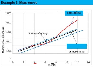
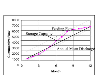
I. Mass curve (Rippl's) method:
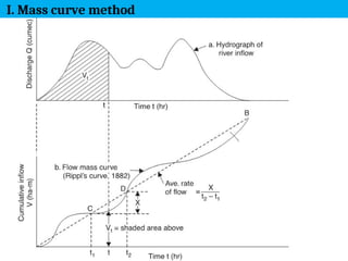
• A mass curve (or mass inflow curve) is a plot of accumulated
flow in a stream against time. It rises continuously as it shows
accumulated flows.
• The slope of the curve at any point indicates the rate of inflow
at that particular time.
• Required rates of draw off from the reservoir are marked by
drawing tangents, having slopes equal to the demand rates, at
the highest points of the mass curve
• If the demand is at a constant rate then the demand curve is a
straight line having its slope equal to the demand rate.
However,
5.2 Methods to determine a reservoir storage capacity.

10. if
the demand is not constant then the demand will be curved 6
indicating a variable rate of demand.

11. 7
I. Mass curve method

12. 8
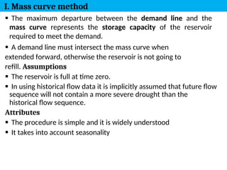
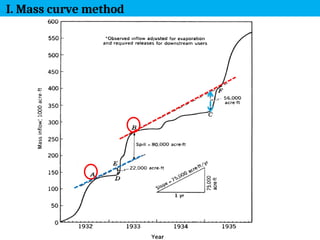
 The maximum departure between the demand line and the
mass curve represents the storage capacity of the reservoir
required to meet the demand.
 A demand line must intersect the mass curve when
extended forward, otherwise the reservoir is not going to
refill. Assumptions
 The reservoir is full at time zero.
 In using historical flow data it is implicitly assumed that future flow
sequence will not contain a more severe drought than the
historical flow sequence.
Attributes
 The procedure is simple and it is widely understood
 It takes into account seasonality
I. Mass curve method

13. 9
I. Mass curve method

14. 10
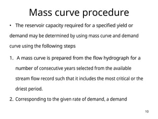
Mass curve procedure
• The reservoir capacity required for a specified yield or
demand may be determined by using mass curve and demand
curve using the following steps
1. A mass curve is prepared from the flow hydrograph for a
number of consecutive years selected from the available
stream flow record such that it includes the most critical or the
driest period.
2. Corresponding to the given rate of demand, a demand

15. 11
curve is prepared.
3. Lines are drawn parallel to the demand curve and tangential to the
high points of the mass curve

16. 12
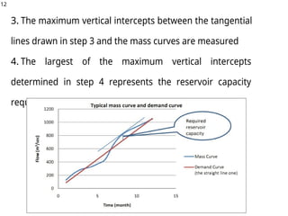
3. The maximum vertical intercepts between the tangential
lines drawn in step 3 and the mass curves are measured
4. The largest of the maximum vertical intercepts
determined in step 4 represents the reservoir capacity
required to satisfy the given demand.

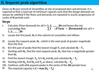
17. IX. The required capacity is C = max (Hk – Tk) 13
𝒊=
𝟏
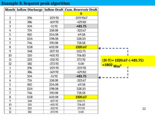
Given an N year record of streamflow at site of proposed dam and demand, it is
required to find a reservoir of minimum capacity such that the design demand can
always be satisfied if the flows and demands are repeated in acyclic progression of
cycles of N periods each.
Steps
I. Calculate (Flow-Demand) for all i = 1, 2, …… , 2N and hence the net
cumulative flow ∑𝒕 (𝑭𝒍𝒐𝒘 − 𝑫𝒆𝒎𝒂𝒏𝒅) for all i =
1, 2, …… , 2N
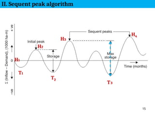
II. Locate the first peak, H1 in the column of cumulative net inflows
III. Locate the sequent peak, H2 , which is the next peak of greater magnitude
than the first.
IV. B/n this pair of peaks find the lowest trough T1 and calculate H1 – T1.
V. Starting with H2, find the next sequent peak, H3, that has a magnitude greater
than H2.
VI. Find the lowest trough, T2, b/n H2 and H3 and calculate H2 – T2.
VII. Starting with H3, find H4 and T3 as above; calculate H3 – T3.
VIII. Continue until all k sequent peaks in the series of the 2N periods have
II. Sequent peak algorithm

18. IX. The required capacity is C = max (Hk – Tk) 14
been found.

19. 15
H4
3
H2
H1
T1
T2
3
II. Sequent peak algorithm
H
T

20. 16
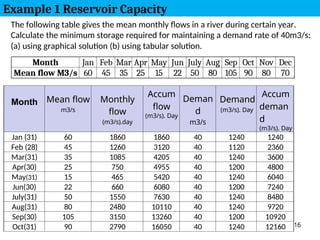
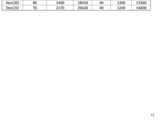
The following table gives the mean monthly flows in a river during certain year.
Calculate the minimum storage required for maintaining a demand rate of 40m3/s:
(a) using graphical solution (b) using tabular solution.
Month Jan Feb Mar Apr May Jun July Aug Sep Oct Nov Dec
Mean flow M3/s 60 45 35 25 15 22 50 80 105 90 80 70
Month Mean flow
m3/s
Monthly
flow
(m3/s).day
Accum
flow
(m3/s). Day
Deman
d
m3/s
Demand
(m3/s). Day
Accum
deman
d
(m3/s). Day
Jan (31) 60 1860 1860 40 1240 1240
Feb (28) 45 1260 3120 40 1120 2360
Mar(31) 35 1085 4205 40 1240 3600
Apr(30) 25 750 4955 40 1200 4800
May(31) 15 465 5420 40 1240 6040
Jun(30) 22 660 6080 40 1200 7240
July(31) 50 1550 7630 40 1240 8480
Aug(31) 80 2480 10110 40 1240 9720
Sep(30) 105 3150 13260 40 1200 10920
Oct(31) 90 2790 16050 40 1240 12160
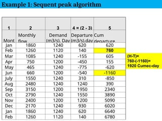
Example 1 Reservoir Capacity

21. 17
Nov(30) 80 2400 18450 40 1200 13360
Dec(31) 70 2170 20620 40 1240 14600

22. 25000
20000
15000
Storage Capacity
10000
5000 Cum_Demand
0
0 2 4 6 8 10 12 14
Month
Example 1: Mass curve
Cum_Inflow
Cummulative
discharge

23. Mass curve Demand curve 15

24. 1 2 3 4 = (2 - 3) 5
Mont
Monthly
flow
Demand
(m3/s). Day
Departure
(m3/s).day
Cum
departure
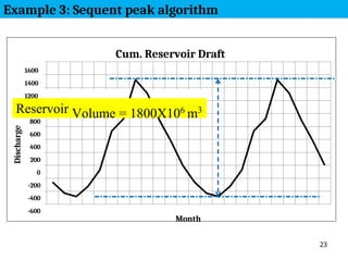
Jan 1860 1240 620 620
Feb 1260 1120 140 760
Mar 1085 1240 -155 605 (H-T)=
760-(-1160)=
1920 Cumec-day
Apr 750 1200 -450 155
May 465 1240 -775 -620
Jun 660 1200 -540 -1160
July 1550 1240 310 -850
Aug 2480 1240 1240 390
Sep 3150 1200 1950 2340
Oct 2790 1240 1550 3890
Nov 2400 1200 1200 5090
Dec 2170 1240 930 6020
Jan 1860 1240 620 6640
Feb 1260 1120 140 6780
Example 1: Sequent peak algorithm

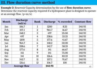
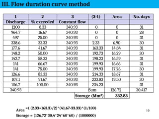
25. Example 2: Reservoir Capacity determination by the use of flow duration curve.
Determine the reservoir capacity required if a hydropower plant is designed to operate
at an average flow. (p=m/n)
Month
Discharge
(m3/s)
Rank Discharge % exceeded Constant flow
Jan 106.7 1 1200 8.33 340.93
Feb 107.1 2 964.7 16.67 340.93
Mar 148.2 3 497 25.00 340.93
Apr 497 4 338.6 33.33 340.93
May 1200 5 177.6 41.67 340.93
Jun 964.7 6 148.2 50.00 340.93
Jul 338.6 7 142.7 58.33 340.93
Aug 177.6 8 141 66.67 340.93
Sep 141 9 141 75.00 340.93
Oct 141 10 126.6 83.33 340.93
Nov 142.7 11 107.1 91.67 340.93
Dec 126.6 12 106.7 100 340.93
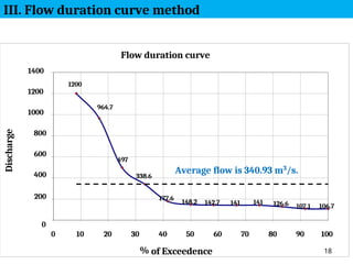
Average flow 340.93 17
III. Flow duration curve method

26. 1400
1200
1000
1200
964.7
Flow duration curve
800
600
400
497
338.6
Average flow is 340.93 m3
/s.
200 177.6
148.2 142.7 141 141 126.6 107.1 106.7
0
0 10 20 30 40 50 60 70 80 90 100
% of Exceedence 18
III. Flow duration curve method
Discharge

27. 1 2 3 (3-1) Area No. days
Discharge % exceeded Constant flow
1200 8.33 340.93 0 0 31
964.7 16.67 340.93 0 0 28
497 25.00 340.93 0 0 31
338.6 33.33 340.93 2.33 6.90 30
177.6 41.67 340.93 163.33 14.84 31
148.2 50.00 340.93 192.73 16.29 30
142.7 58.33 340.93 198.23 16.59 31
141 66.67 340.93 199.93 16.66 31
141 75.00 340.93 199.93 17.26 30
126.6 83.33 340.93 214.33 18.67 31
107.1 91.67 340.93 233.83 19.50 30
106.7 100.00 340.93 234.23 31
340.93 Sum 126.72 30.417
Storage (Mm3) 332.83
Area
=( (2.33+163.3)/2)*(41.67-33.33)*(1/100)
19
Storage = (126.72*30.4*24*60*60) / (1000000)
III. Flow duration curve method

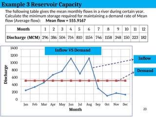
28. The following table gives the mean monthly flows in a river during certain year.
Calculate the minimum storage required for maintaining a demand rate of Mean
flow (Average flow): Mean flow = 555.9167
Month 1 2 3 4 5 6 7 8 9 10 11 12
Discharge (MCM) 296 386 504 714 810 1154 746 1158 348 150 223 182
1400
1200
1000
800
600
400
200
0
Jan Feb Mar Apr May Jun Jul Aug Sep Oct Nov Dec
Month
Inflow
Demand
20
Inflow VS Demand
Example 3 Reservoir Capacity
Discharge

29. 8000
7000
6000
5000
4000
3000
2000
1000
0
Feeding Flow
Storage Capacity
Annual Mean Discharge
0 3 6 9 12
Month
Cummulative
Flow
Rate

30. 21
Example 3: Mass curve

31. 22
Month Inflow Discharge Inflow-Draft Cum. Reservoir Draft
0
1 296 -259.92 -259.9167
2 386 -169.92 -429.83
3 504 -51.92 -481.75
4 714 158.08 -323.67
5 810 254.08 -69.58
6 1154 598.08 528.50
7 746 190.08 718.58
8 1158 602.08 1320.67
9 348 -207.92 1112.75
10 150 -405.92 706.83
11 223 -332.92 373.92
12 182 -373.92 0.00
1 296 -259.92 -259.92
2 386 -169.92 -429.83
3 504 -51.92 -481.75
4 714 158.08 -323.67
5 810 254.08 -69.58
6 1154 598.08 528.50
7 746 190.08 718.58
8 1158 602.08 1320.67
9 348 -207.92 1112.75
10 150 -405.92 706.83
11 223 -332.92 373.92
12 182 -373.92 0.00
Example 3: Sequent peak algorithm
(H-T)= 1320.67-(-481.75)
=1802 Mm3

32. 23
1000
Reservoir Volume = 1800X106
m3
1600
1400
1200
Cum. Reservoir Draft
800
600
400
200
0
-200
-400
-600
Month
Example 3: Sequent peak algorithm
Discharge

33. 24
• A river entering a water reservoir will loose its capacity to
transport sediments. b/c water velocity decreases, together
with the shear stress on the bed. The sediments will therefore
deposit in the reservoir and decrease its volume.
• In the design of dam, it is important to assess the magnitude
of sediment deposition in the reservoir. The problem can be
divided In two parts:
1. How much sediments enter the reservoir
2. What is the trap efficiency of the reservoir
• In a detailed study, the sediment size distributions also have
to be determined for question 1.
5.3. Reservoirs and sediments

34. 25
• Question 2 may also involve determining the location of the
deposits and the concentration and grain size distribution of the
sediments entering the water intakes.

35. 26
Trap efficiency

36. 27

37. 28
The structure of a reservoir

38. 29
Reservoir structure

39. 30
Spillway

40. 31

41. 32
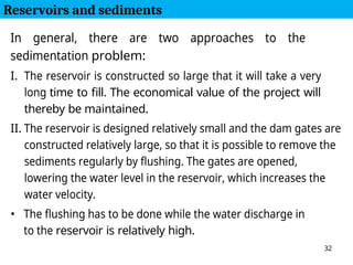
In general, there are two approaches to the
sedimentation problem:
I. The reservoir is constructed so large that it will take a very
long time to fill. The economical value of the project will
thereby be maintained.
II. The reservoir is designed relatively small and the dam gates are
constructed relatively large, so that it is possible to remove the
sediments regularly by flushing. The gates are opened,
lowering the water level in the reservoir, which increases the
water velocity.
• The flushing has to be done while the water discharge in
to the reservoir is relatively high.
Reservoirs and sediments

42. 33
• A long and narrow reservoir will therefore be more
effectively flushed than a short and wide geometry. For the
later, the sediment deposits may remain on the sides.

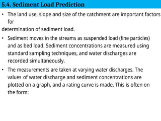
43. • The land use, slope and size of the catchment are important factors
for
determination of sediment load.
• Sediment moves in the streams as suspended load (fine particles)
and as bed load. Sediment concentrations are measured using
standard sampling techniques, and water discharges are
recorded simultaneously.
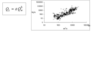
• The measurements are taken at varying water discharges. The
values of water discharge and sediment concentrations are
plotted on a graph, and a rating curve is made. This is often on
the form:
5.4. Sediment Load Prediction

44. 30

45. 31
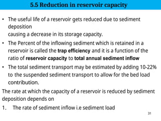
• The useful life of a reservoir gets reduced due to sediment
deposition
causing a decrease in its storage capacity.
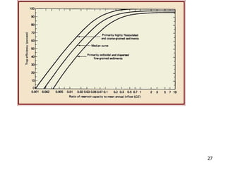
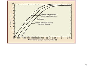
• The Percent of the inflowing sediment which is retained in a
reservoir is called the trap efficiency and it is a function of the
ratio of reservoir capacity to total annual sediment inflow
• The total sediment transport may be estimated by adding 10-22%
to the suspended sediment transport to allow for the bed load
contribution.
The rate at which the capacity of a reservoir is reduced by sediment
deposition depends on
1. The rate of sediment inflow i.e sediment load
5.5 Reduction in reservoir capacity

46. 32
2. The percentage of the sediment inflow trapped in the reservoir,
i.e.
trap efficiency
3. The density of the deposited sediment.

47. 33
Trap efficiency

48. 34

49. 33
Sediment Management
 Catchment Vegetation
 Construction of coffer dams/low height barriers
 Flushing and desilting of sediments
 Low level outlets / sediment sluicing

50. Catchment vegetation

51. 34

52. Wooden barriers

53. 35

54. Wooden barriers

55. 36

56. Stepped watershed for sediment
control

57. 37

58. Flushing of sediments from reservoir

59. 38

60. Sediment sluicing

61. 39

62. Sediment sluicing

63. 40

64. 41
Thank You !!!