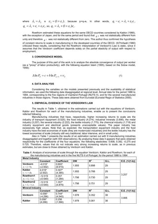
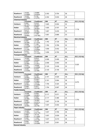
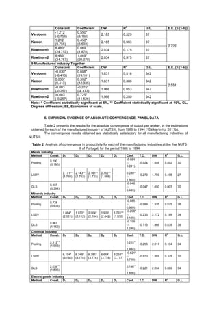
THE KEYNESIAN AND THE CONVERGENCE THEORIES IN THE

THE KEYNESIAN AND THE CONVERGENCE THEORIES IN THE
PORTUGUESE MANUFACTURED INDUSTRY
Vitor João Pereira Domingues Martinho

Unidade de I&D do Instituto Politécnico de Viseu
Av. Cor. José Maria Vale de Andrade
Campus Politécnico
3504 - 510 Viseu
(PORTUGAL)
e-mail: vdmartinho@esav.ipv.pt

ABSTRACT

This work aims to test the Verdoorn Law, with the alternative specifications of (1)Kaldor (1966),
for the five Portuguese regions (NUTS II), from 1986 to 1994. It is intended to test, yet in this work, the
alternative interpretation of (2)Rowthorn (1975) about the Verdoorn's Law for the same regions and period.
The results of this study are about each one of the manufactured industries operating in the Portuguese
regions. The aim of this paper is, also, to present a further contribution to the analysis of absolute
convergence, associated with the neoclassical theory, of the manufactured industry productivity at regional
level and for the period from 1986 to 1994.

Keywords: Verdoorn law; convergence theories; panel data; manufactured industries;
Portuguese regions.

1. INTRODUCTION

Kaldor rediscovered the Verdoorn law in 1966 and since then this law has been tested in several
ways, using specifications, samples and different periods (3)(Martinho, 2011a). However, the conclusions
drawn differ, some of them rejecting the Law of Verdoorn and other supporting its validity. (4)Kaldor (1966,
1967) in his attempt to explain the causes of the low rate of growth in the UK, reconsidering and
empirically investigating Verdoorn's Law, found that there is a strong positive relationship between the
growth of labor productivity (p) and output (q), i.e. p = f (q). Or alternatively between employment growth
(e) and the growth of output, ie, e = f (q).
Another interpretation of Verdoorn's Law, as an alternative to the Kaldor, is presented by
(5)Rowthorn (1975, 1979). Rowthorn argues that the most appropriate specification of Verdoorn's Law is
the ratio of growth of output (q) and the growth of labor productivity (p) with employment growth (e), i.e., q
= f (e) and p = f (e), respectively (as noted above, the exogenous variable in this case is employment). On
the other hand, Rowthorn believes that the empirical work of Kaldor (1966) for the period 1953-54 to 1963-
64 and the (6)Cripps and Tarling (1973) for the period 1951 to 1965 that confirm Kaldor's Law, not can be
accepted since they are based on small samples of countries, where extreme cases end up like Japan
have great influence on overall results.
(7)Islam (1995) developed a model about the convergence issues, for panel data, based on the
(8)Solow model, (1956).

2. ALTERNATIVE SPECIFICATIONS OF VERDOORN'S LAW

The hypothesis of increasing returns to scale in industry was initially tested by Kaldor (1966)
using the following relations:

pi  a  bqi , Verdoorn law (1)
ei  c  dqi , Kaldor law (2)

where pi, qi and ei are the growth rates of labor productivity, output and employment in the industrial
sector in the economy i.

On the other hand, the mathematical form of Rowthorn specification is as follows:

pi  1   1ei , firts equation of Rowthorn (3)
qi  2   2 ei , second equation of Rowthorn (4)

where 1  2 e  2  (1   1 ) , because pi=qi-ei. In other words, qi  ei  1   1ei ,
qi  1  ei   1ei , so, qi  1  (1   1 )ei .

Rowthorn estimated these equations for the same OECD countries considered by Kaldor (1966),
with the exception of Japan, and for the same period and found that  2 was not statistically different from
unity and therefore 1 was not statistically different from zero. This author thus confirmed the hypothesis
of constant returns to scale in manufacturing in the developed countries of the OECD. (9)Thirlwall (1980)
criticized these results, considering that the Rowthorn interpretation of Verdoorn's Law is static, since it
assumes that the Verdoorn coefficient depends solely on the partial elasticity of output with respect to
employment.

3. CONVERGENCE MODEL

The purpose of this part of the work is to analyze the absolute convergence of output per worker
(as a "proxy" of labor productivity), with the following equation Islam (1995), based on the Solow model,
1956):

 ln Pit  c  b ln Pi ,t 1   it (1)

4. DATA ANALYSIS

Considering the variables on the models presented previously and the availability of statistical
information, we used the following data disaggregated at regional level. Annual data for the period 1986 to
1994, corresponding to the five regions of mainland Portugal (NUTS II), and for the several manufactured
industries in those regions. These data were obtained from Eurostat (Eurostat Regio of Statistics 2000).

5. EMPIRICAL EVIDENCE OF THE VERDOORN'S LAW

The results in Table 1, obtained in the estimations carried out with the equations of Verdoorn,
Kaldor and Rowthorn for each of the manufacturing industries, enable us to present the conclusions
referred following.
Manufacturing industries that have, respectively, higher increasing returns to scale are the
industry of transport equipment (5.525), the food industry (4.274), industrial minerals (3.906), the metal
industry (3.257), the several industry (2.222), the textile industry (1.770), the chemical industry (1.718) and
industry equipment and electrical goods (presents unacceptable values). The paper industry has
excessively high values. Note that, as expected, the transportation equipment industry and the food
industry have the best economies of scale (they are modernized industries) and the textile industry has the
lowest economies of scale (industry still very traditional, labor intensive, and in small units).
Also in Table 1 presents the results of an estimation carried out with 9 manufacturing industries
disaggregated and together (with 405 observations). By analyzing these data it appears that were obtained
respectively for the coefficients of the four equations, the following elasticities: 0.608, 0.392, -0.275 and
0.725. Therefore, values that do not indicate very strong increasing returns to scale, as in previous
estimates, but are close to those obtained by Verdoorn and Kaldor.

Table 1: Analysis of economies of scale through the equation Verdoorn, Kaldor and Rowthorn, for each of
the manufacturing industries and in the five NUTS II of Portugal, for the period 1986 to 1994
Metal Industry
2
Constant Coefficient DW R G.L. E.E. (1/(1-b))
Verdoorn -4.019* 0.693*
pi  a  bqi
1.955 0.898 29
(-2.502) (9.915)
Kaldor 4.019* 0.307*
ei  c  dqi
1.955 0.788 29
(2.502) (4.385)
Rowthorn1 3.257
-12.019 0.357
pi  1   1ei 1.798 0.730 29
(-0.549) (1.284)
Rowthorn2 -12.019 1.357*
qi  2   2 ei 1.798 0.751 29
(-0.549) (4.879)
Mineral Industry
2
-0.056* 0.744*
Verdoorn 1.978 0.352 38
(-4.296) (4.545)
3.906
0.056* 0.256
Kaldor 1.978 0.061 38
(4.296) (1.566)

-0.023 -0.898*
Rowthorn1 2.352 0.704 38
(-0.685) (-9.503)
-0.023 0.102
Rowthorn2 2.352 0.030 38
(-0.685) (1.075)
Chemical Industry
2
0.002 0.418*
Verdoorn 1.825 0.554 34
(0.127) (6.502)
-0.002 0.582*
Kaldor 1.825 0.707 34
(-0.127) (9.052)
1.718
9.413* 0.109
Rowthorn1 1.857 0.235 33
(9.884) (0.999)
9.413* 1.109*
Rowthorn2 1.857 0.868 33
(9.884) (10.182)
Electrical Industry
2
0.004 -0.126
Verdoorn 1.762 0.128 32
(0.208) (-1.274)
-0.004 1.126*
Kaldor 1.762 0.796 32
(-0.208) (11.418)
---
0.019 -0.287*
Rowthorn1 1.659 0.452 32
(1.379) (-4.593)
0.019 0.713*
Rowthorn2 1.659 0.795 32
(1.379) (11.404)
Transport Industry
2
-0.055* 0.819*
Verdoorn 2.006 0.456 38
(-2.595) (5.644)
0.055* 0.181
Kaldor 2.006 0.040 38
(2.595) (1.251)
5.525
-0.001 -0.628*
Rowthorn1 2.120 0.436 32
(-0.029) (-3.938)
-0.001 0.372*
Rowthorn2 2.120 0.156 32
(-0.029) (2.336)
Food Industry
2
0.006 0.766*
Verdoorn 2.191 0.526 38
(0.692) (6.497)
-0.006 0.234**
Kaldor 2.191 0.094 38
(-0.692) (1.984)
4.274
0.048* -0.679*
Rowthorn1 1.704 0.324 38
(2.591) (-4.266)
0.048* 0.321*
Rowthorn2 1.704 0.097 38
(2.591) (2.018)
Textile Industry
2
-0.008 0.435*
Verdoorn 2.117 0.271 34
(-0.466) (3.557)
0.008 0.565*
Kaldor 2.117 0.386 34
(0.466) (4.626)
1.770
0.002 -0.303*
Rowthorn1 1.937 0.136 34
(0.064) (-2.311)
0.002 0.697*
Rowthorn2 1.937 0.454 34
(0.064) (5.318)
Paper Industry
2
-0.062* 1.114*
Verdoorn 1.837 0.796 38
(-3.981) (12.172)
0.062* -0.114
Kaldor 1.837 0.039 38
(3.981) (-1.249)

0.028 -1.053*
Rowthorn1 1.637 0.310 38
(1.377) (-4.134)
0.028 -0.053
Rowthorn2 1.637 0.001 38
(1.377) (-0.208)
Several Industry

2
-1.212 0.550*
Verdoorn 2.185 0.529 37
(-0.756) (8.168)
1.212 0.450*
Kaldor 2.185 0.983 37
(0.756) (6.693)
2.222
8.483* 0.069
Rowthorn1 2.034 0.175 37
(24.757) (1.878)
8.483* 1.069*
Rowthorn2 2.034 0.975 37
(24.757) (29.070)
9 Manufactured Industry Together
2
-0.030* 0.608*
Verdoorn 1.831 0.516 342
(-6.413) (19.101)
0.030* 0.392*
Kaldor 1.831 0.308 342
(6.413) (12.335)
2.551
-0.003 -0.275*
Rowthorn1 1.968 0.053 342
(-0.257) (-4.377)
-0.003 0.725*
Rowthorn2 1.968 0.280 342
(-0.257) (11.526)
Note: * Coefficient statistically significant at 5%, ** Coefficient statistically significant at 10%, GL,
Degrees of freedom; EE, Economies of scale.

6. EMPIRICAL EVIDENCE OF ABSOLUTE CONVERGENCE, PANEL DATA

Table 2 presents the results for the absolute convergence of output per worker, in the estimations
obtained for each of the manufactured industry of NUTS II, from 1986 to 1994 (10)(Martinho, 2011b).
The convergence results obtained are statistically satisfactory for all manufacturing industries of
NUTS II.

Table 2: Analysis of convergence in productivity for each of the manufacturing industries at the five NUTS
II of Portugal, for the period 1986 to 1994
Metals industry
Method Const. D1 D2 D3 D4 D5 Coef. T.C. DW R2 G.L.
-0.024
0.190
Pooling (- -0.024 1.646 0.002 30
(0.190)
0.241)
-
2.171** 2.143** 2.161** 2.752** 0.239**
LSDV --- -0.273 1.759 0.198 27
(1.769) (1.753) (1.733) (1.988) (-
1.869)
-0.046
0.407
GLS (- -0.047 1.650 0.007 30
(0.394)
0.445)
MInerals industry
-0.085
0.738
Pooling (- -0.089 1.935 0.025 38
(0.903)
0.989)
-0.208*
1.884* 1.970* 2.004* 1.926* 1.731**
LSDV (- -0.233 2.172 0.189 34
(2.051) (2.112) (2.104) (2.042) (1.930)
2.129)
-0.109
0.967
GLS (- -0.115 1.966 0.039 38
(1.162)
1.246)
Chemical industry
-
2.312** 0.225**
Pooling -0.255 2.017 0.104 34
(1.992) (-
1.984)
-0.621*
6.104* 6.348* 6.381* 6.664* 6.254*
LSDV (- -0.970 1.959 0.325 30
(3.750) (3.778) (3.774) (3.778) (3.777)
3.769)
-
2.038** 0.198**
GLS -0.221 2.034 0.089 34
(1.836) (-
1.826)
Electric goods industry

-0.083
0.781
Pooling (- -0.087 1.403 0.016 38
(0.789)
0.784)
-0.381*
3.634* 3.552* 3.673* 3.636* 3.429*
LSDV (- -0.480 1.259 0.167 34
(2.363) (2.360) (2.362) (2.376) (2.324)
2.355)
-0.025
0.242
GLS (- -0.025 1.438 0.002 38
(0.285)
0.279)
Transport equipments industry
-0.464*
4.460*
Pooling (- -0.624 2.258 0.206 38
(3.110)
3.136)
-0.871*
8.061* 8.526* 8.614* 8.696* 8.077*
LSDV (- -2.048 2.049 0.429 34
(4.948) (5.007) (4.986) (4.998) (4.961)
5.014)
-0.596*
5.735*
GLS (- -0.906 2.159 0.276 38
(3.780)
3.807)
Food industry
-0.027
0.314
Pooling (- -0.027 1.858 0.005 38
(0.515)
0.443)
-0.274*
2.841* 2.777* 2.899* 2.617* 2.593*
LSDV (- -0.320 1.786 0.198 34
(2.555) (2.525) (2.508) (2.471) (2.470)
2.469)
-0.005
0.090
GLS (- -0.005 1.851 0.001 38
(0.166)
0.085)
Textile industry
-0.462*
4.276*
Pooling (- -0.620 1.836 0.388 34
(4.639)
4.645)
-0.595*
5.556* 5.487* 5.506* 5.561* 5.350*
LSDV (- -0.904 1.816 0.431 30
(4.288) (4.276) (4.272) (4.253) (4.431)
4.298)
-0.347*
3.212*
GLS (- -0.426 1.848 0.542 34
(6.336)
6.344)
Paper industry
-0.271*
2.625*
Pooling (- -0.316 1.534 0.128 38
(2.332)
2.366)
-0.382*
3.703* 3.847* 3.837* 3.684* 3.521*
LSDV (- -0.481 1.516 0.196 34
(2.803) (2.840) (2.813) (2.812) (2.782)
2.852)
-
1.939** 0.201**
GLS -0.224 1.556 0.089 38
(1.888) (-
1.924)
Several industry
-0.605*
5.518*
Pooling (- -0.929 2.121 0.297 38
(4.004)
4.004)
-0.847*
7.802* 7.719* 7.876* 7.548* 7.660*
LSDV (- -1.877 2.024 0.428 34
(5.036) (5.022) (5.033) (5.023) (5.018)
5.032)
-0.664*
6.053*
GLS (- -1.091 2.081 0.328 38
(4.308)
4.309)

7. CONCLUSIONS

At the level of estimates made for manufactured industries, it appears that those with,
respectively, higher dynamics are the transport equipment industry, food industry, minerals industrial,
metals industry, the several industries, the textile industry, chemical industry and equipment and electrical
goods industry. The paper industry has excessively high values.

The signs of absolute convergence are different from one manufactured industries to another, but
there is a curious results for the equipment transport industry, because present strong evidence of
absolute convergence and we know that this industry is a dynamic sector.
So, we can that the strong increasing returns to scale in the same industries (like the transport
equipment industry) are not enough to avoid the convergence of this industries.

8. REFERENCES

1. N. Kaldor. Causes of the Slow Rate of Economics of the UK. An Inaugural Lecture. Cambridge:
Cambridge University Press, 1966.
2. R.E. Rowthorn. What Remains of Kaldor Laws? Economic Journal, 85, 10-19 (1975).
3. V.J.P.D. Martinho. The Verdoorn law in the Portuguese regions: a panel data analysis. MPRA Paper
32186, University Library of Munich, Germany (2011a).
4. N. Kaldor. Strategic factors in economic development. Cornell University, Itaca, 1967.
5. R.E. Rowthorn. A note on Verdoorn´s Law. Economic Journal, Vol. 89, pp: 131-133 (1979).
6. T.F. Cripps and R.J. Tarling. Growth in advanced capitalist economies: 1950-1970. University of
Cambridge, Department of Applied Economics, Occasional Paper 40, 1973.
7. N. Islam. Growth Empirics : A Panel Data Approach. Quarterly Journal of Economics, 110, 1127-1170
(1995).
8. R. Solow. A Contribution to the Theory of Economic Growth. Quarterly Journal of Economics (1956).
9. A.P. Thirlwall. Regional Problems are “Balance-of-Payments” Problems. Regional Studies, Vol. 14, 419-
425 (1980).
10. V.J.P.D. Martinho. Sectoral convergence in output per worker between Portuguese regions. MPRA
Paper 32269, University Library of Munich, Germany (2011b).

THE KEYNESIAN AND THE CONVERGENCE THEORIES IN THE

More Related Content

What's hot

Viewers also liked

Similar to THE KEYNESIAN AND THE CONVERGENCE THEORIES IN THE

More from Vítor João Pereira Domingues Martinho

Recently uploaded

THE KEYNESIAN AND THE CONVERGENCE THEORIES IN THE