Decision tree, algorithm,DSA, optimal,design algorithm

1. MODULE 5
Decision Trees, Deterministic Polynomial (P), Non-
Deterministic Polynomial (NP) & NP complete problems.
Backtracking: N Queens problem, Branch & Bound:
Travelling Salesman problem, Assignment problem

2. Introduction to Decision Trees
• What is a Decision Tree?
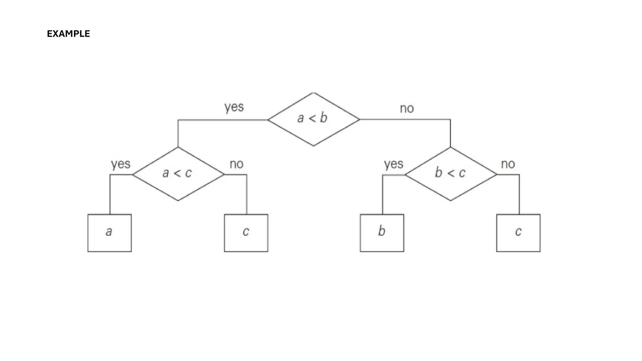
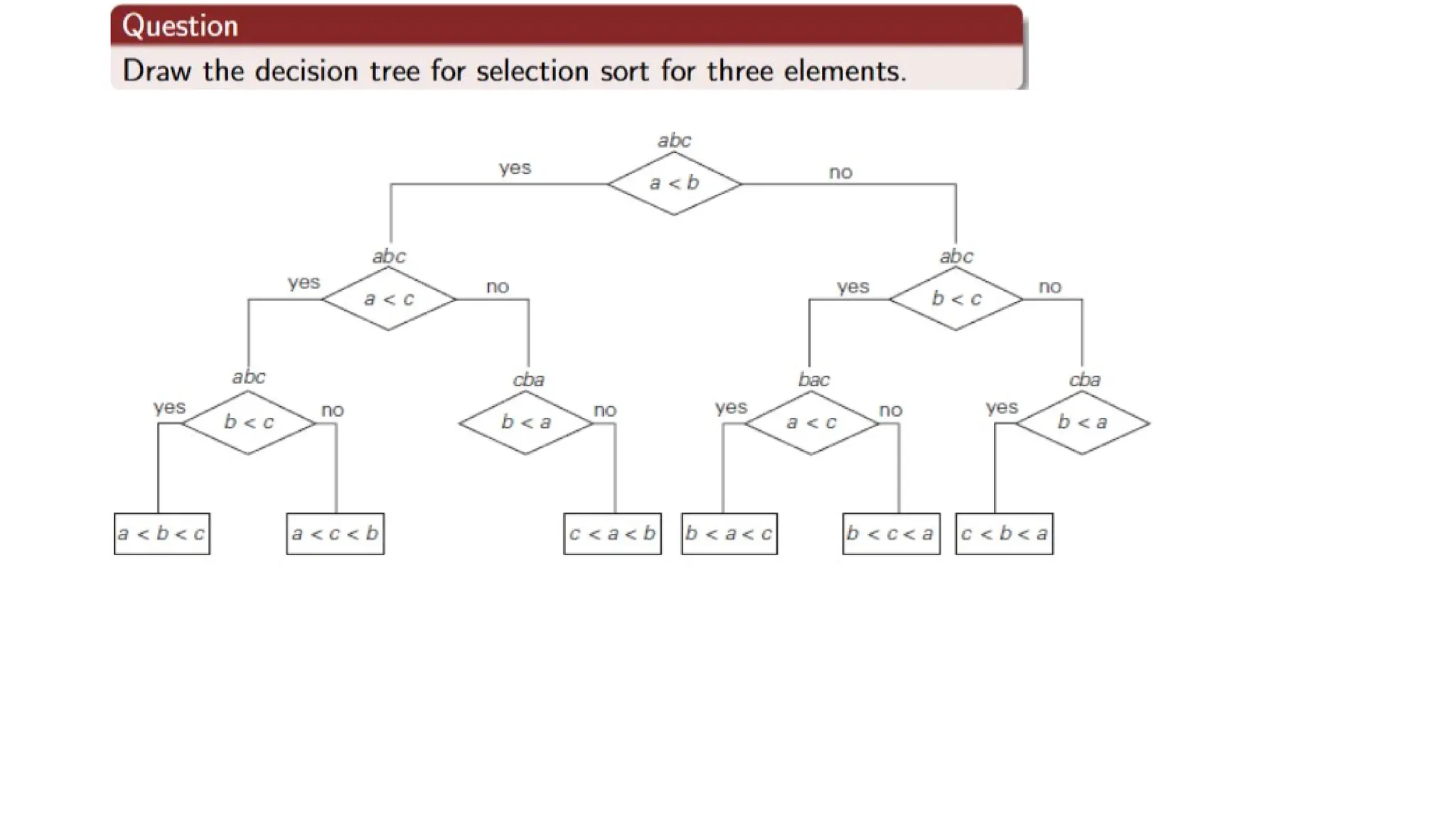
A binary tree that represents the sequence of comparisons made by an
algorithm, with each internal node indicating a key comparison.
• Why Use Decision Trees?
They help analyze the performance and complexity of comparison-based
algorithms like sorting and searching.
• Key Insights:
• Tree height h determines the worst-case number of comparisons.
• Minimum height h≥[log2n], where n is the number of outcomes (leaves).
• Maximum leaves for height h: 2h
.

3. EXAMPLE

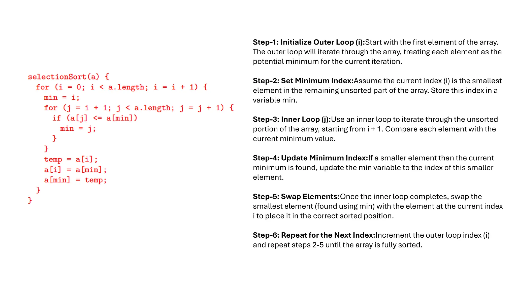
5. Step-1: Initialize Outer Loop (i):Start with the first element of the array.
The outer loop will iterate through the array, treating each element as the
potential minimum for the current iteration.
Step-2: Set Minimum Index:Assume the current index (i) is the smallest
element in the remaining unsorted part of the array. Store this index in a
variable min.
Step-3: Inner Loop (j):Use an inner loop to iterate through the unsorted
portion of the array, starting from i + 1. Compare each element with the
current minimum value.
Step-4: Update Minimum Index:If a smaller element than the current
minimum is found, update the min variable to the index of this smaller
element.
Step-5: Swap Elements:Once the inner loop completes, swap the
smallest element (found using min) with the element at the current index
i to place it in the correct sorted position.
Step-6: Repeat for the Next Index:Increment the outer loop index (i)
and repeat steps 2-5 until the array is fully sorted.

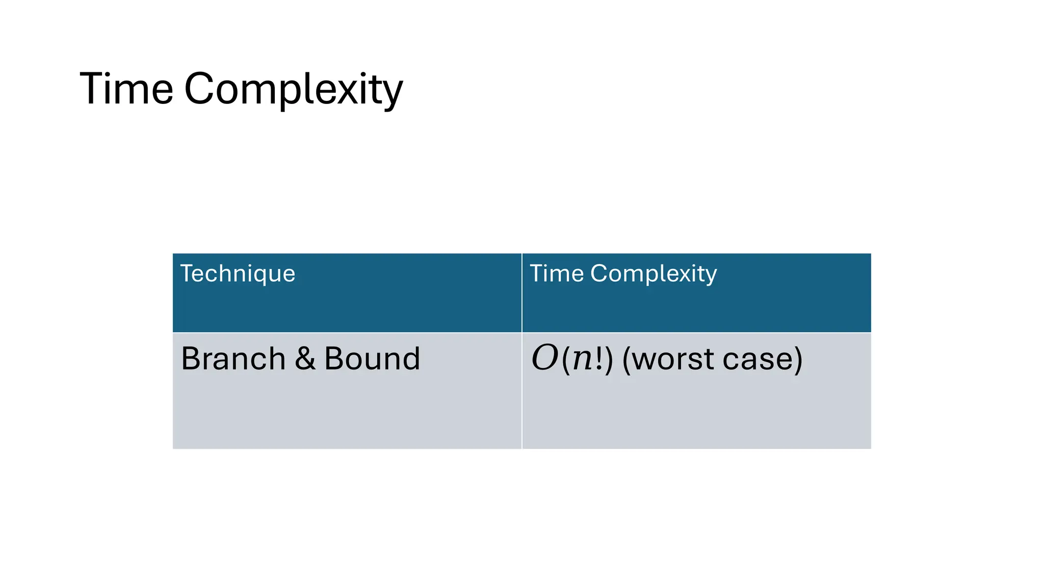
6. Time Complexity
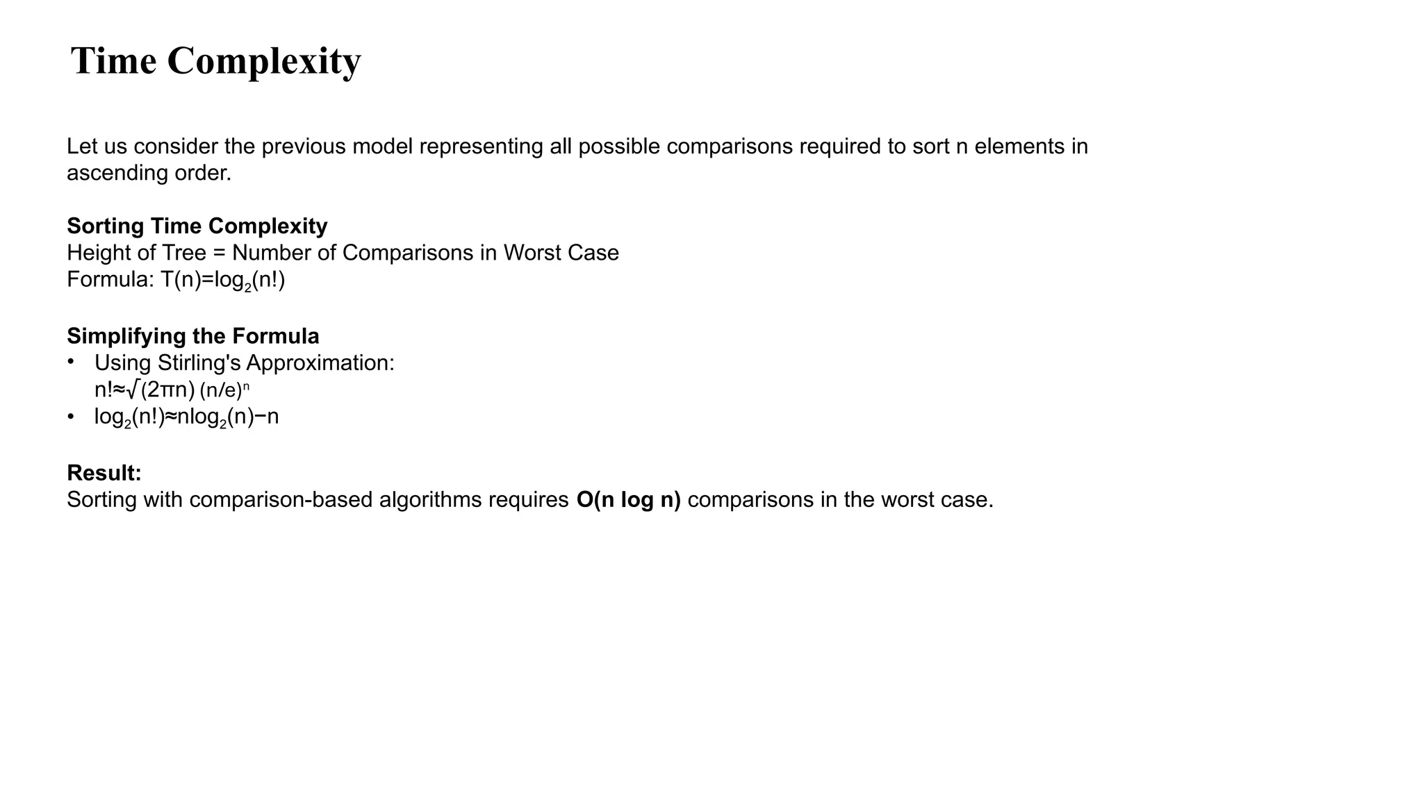
Let us consider the previous model representing all possible comparisons required to sort n elements in
ascending order.
Sorting Time Complexity
Height of Tree = Number of Comparisons in Worst Case
Formula: T(n)=log2(n!)
Simplifying the Formula
• Using Stirling's Approximation:
n!≈√(2πn) (n/e)n
• log2(n!)≈nlog2(n)−n
Result:
Sorting with comparison-based algorithms requires O(n log n) comparisons in the worst case.

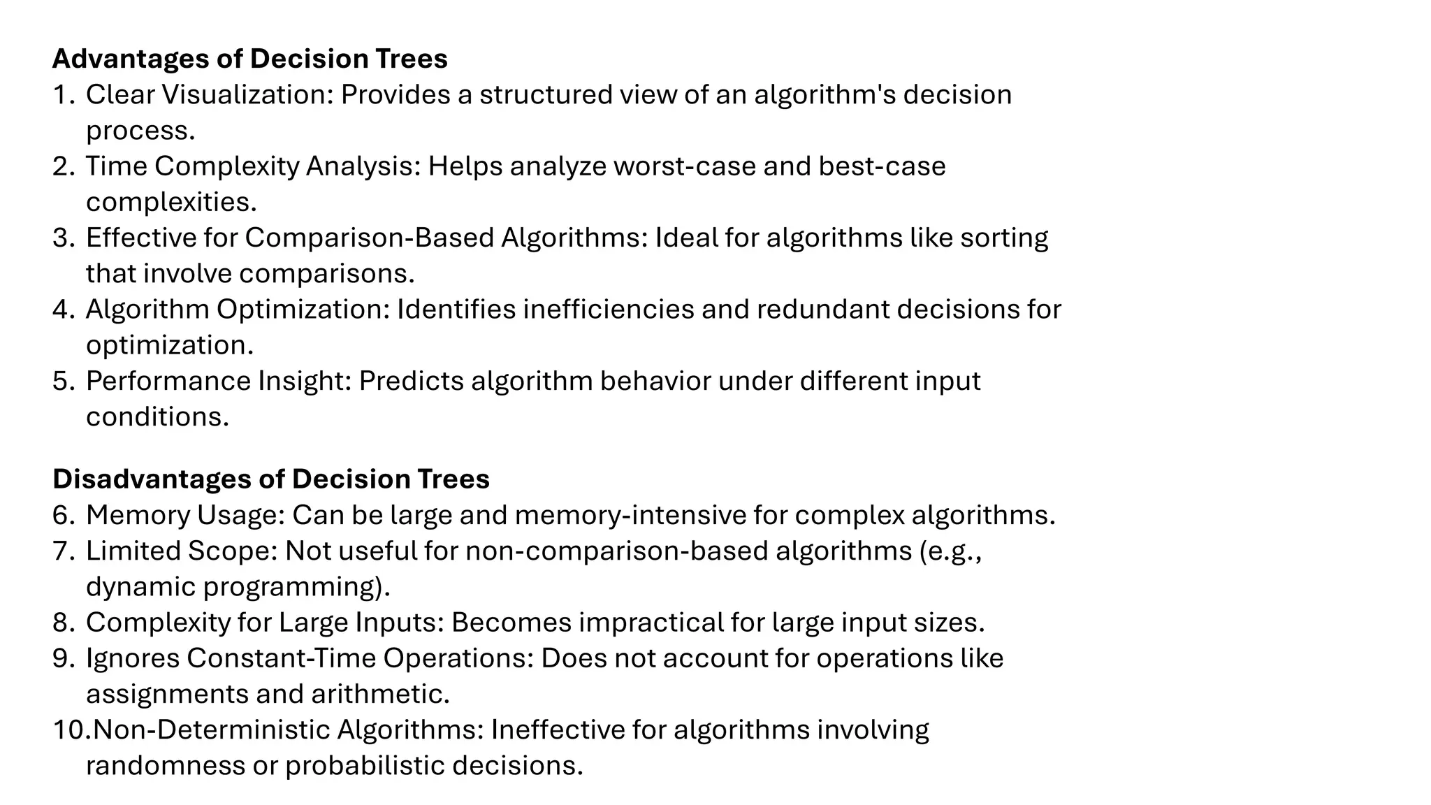
7. Advantages of Decision Trees
1. Clear Visualization: Provides a structured view of an algorithm's decision
process.
2. Time Complexity Analysis: Helps analyze worst-case and best-case
complexities.
3. Effective for Comparison-Based Algorithms: Ideal for algorithms like sorting
that involve comparisons.
4. Algorithm Optimization: Identifies inefficiencies and redundant decisions for
optimization.
5. Performance Insight: Predicts algorithm behavior under different input
conditions.
Disadvantages of Decision Trees
6. Memory Usage: Can be large and memory-intensive for complex algorithms.
7. Limited Scope: Not useful for non-comparison-based algorithms (e.g.,
dynamic programming).
8. Complexity for Large Inputs: Becomes impractical for large input sizes.
9. Ignores Constant-Time Operations: Does not account for operations like
assignments and arithmetic.
10.Non-Deterministic Algorithms: Ineffective for algorithms involving
randomness or probabilistic decisions.

8. Decoding Complexity:
Understanding P, NP, and NP-
Complete Problems

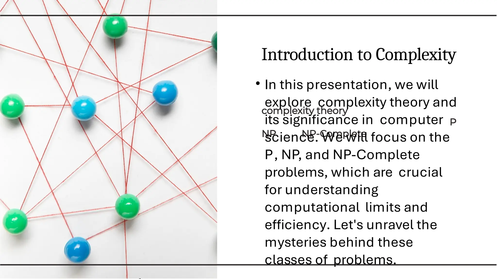
9. Introduction to Complexity
• In this presentation, we will
explore complexity theory and
its significance in computer
science. We will focus on the
P, NP, and NP-Complete
problems, which are crucial
for understanding
computational limits and
efficiency. Let's unravel the
mysteries behind these
classes of problems.

10. What is P?
• P stands for Polynomial time,
representing problems that can be
solved efficiently by algorithms.
These problems have solutions that
can be computed in a time that is a
polynomial function of the input size.
• Examples include sorting and
searching algorithms, which are
fundamental in computer science.

11. NP (Nondeterministic Polynomial
time) includes problems for which a solution can be verified quickly,
even if finding that solution may not be efficient. This class
encompasses many important problems, including the Traveling
Salesman Problem and the Knapsack Problem, highlighting the
challenges of computation.

12. What are NP-Complete Problems?
NP-Complete problems are the
hardest problems in NP, meaning that
if one NP- Complete problem can be
solved efficiently, all NP problems can
be solved efficiently. Examples
include the Clique Problem and Vertex
Cover, which are essential for various
applications in optimization and
decision-making.

13. The P vs NP question is one of the most significant open
problems in computer science. It asks whether every problem
whose solution can be verified quickly (NP) can also be solved
quickly (P).This question has profound implications for
mathematics, cryptography, and algorithm design.

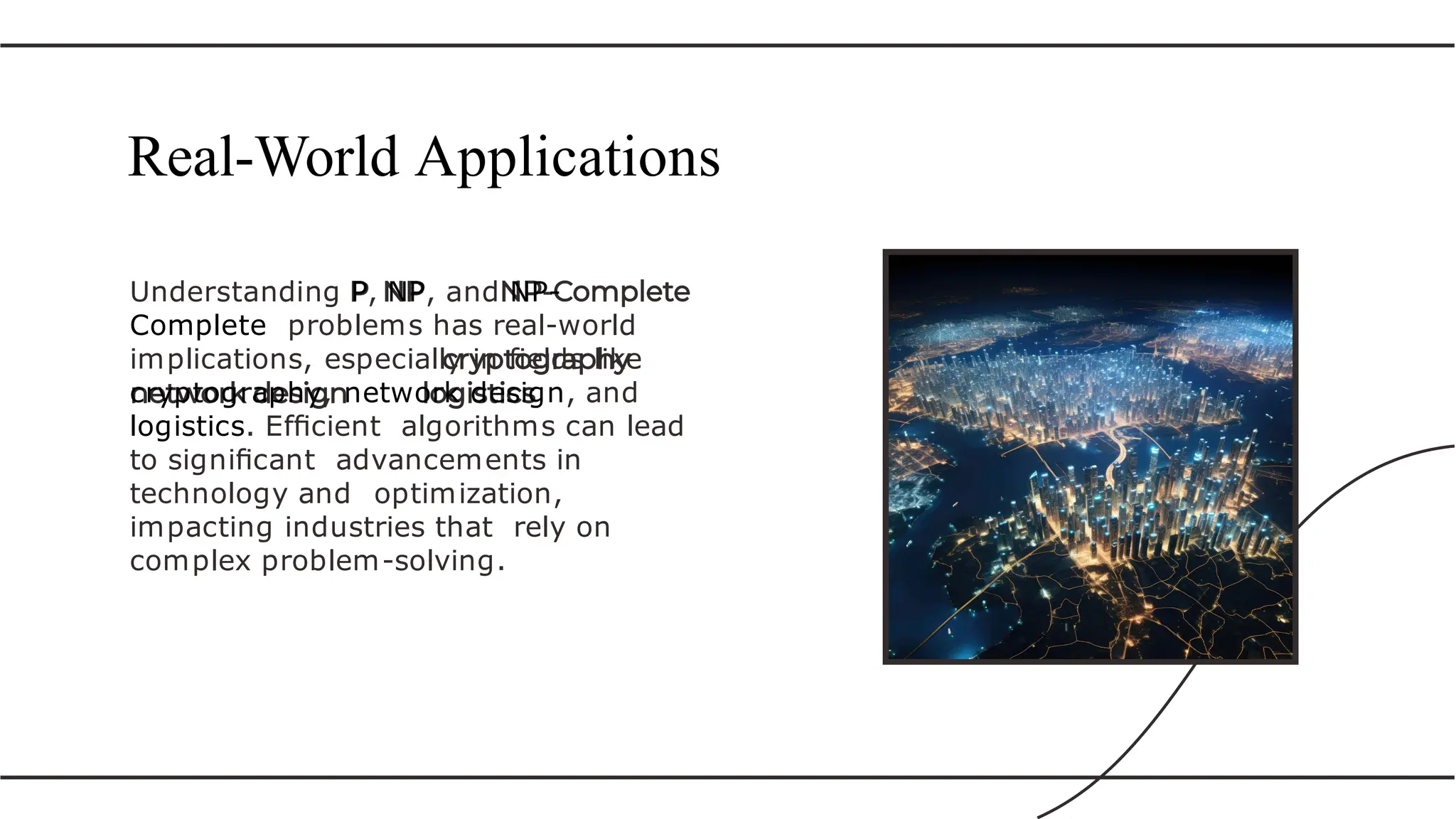
14. Understanding P, NP, and NP-
Complete problems has real-world
implications, especially in fields like
cryptography, network design, and
logistics. Efficient algorithms can lead
to significant advancements in
technology and optimization,
impacting industries that rely on
complex problem-solving.
Real-World Applications

15. Research in complexity theory continues
to evolve, focusing on approximation
algorithms and heuristics for NP-
Complete problems. Researchers are
also exploring quantum computing's
potential to solve these problems more
efficiently, opening new avenues for
breakthroughs in computational theory.
Current Research
Trends

16. In summary, understanding P, NP,
and NP-Complete problems is
crucial for
grasping the limitations and capabilities
of algorithms. As we continue to explore
these concepts, we pave the way for
innovations that can transform
various
fields and enhance our
computational understanding.
Conclusion

17. INTRODUCTION TO BACKTRACKING :
• Backtracking is a recursive algorithmic technique that seeks solutions by
exploring potential candidates incrementally.
• Problem Solving : This technique tries partial solutions and abandons them if
they cannot lead to a viable solution.
• Recursion in Backtracking: Backtracking uses recursion to attempt to build a
solution and backtrack when a conflict arises.
• Viability Check : Each potential position for a queen is checked to ensure it
does not conflict with others already placed.
• Illustration of Backtracking : The N Queens problem serves as a case study
showcasing backtracking's power in solving combinatorial problems.
• Introduction to N Queens Problem : The N Queens problem tasks placing N
queens on an N×N chessboard without any two threatening each other.

18. ALGORITHM
• We create a board of N x N size that stores characters. It will store 'Q' if the queen has been
placed at that position else '.'
• We will create a recursive function called "solve" that takes board and column and all
Boards (that stores all the possible arrangements) as arguments. We will pass the column
as 0 so that we can start exploring the arrangements from column 1.
• In solve function we will go row by row for each column and will check if that particular cell
is safe or not for the placement of the queen, we will do so with the help of isSafe()
function.
• For each possible cell where the queen is going to be placed, we will first check isSafe()
function.
• If the cell is safe, we put 'Q' in that row and column of the board and again call the solve
function by incrementing the column by 1.
• Whenever we reach a position where the column becomes equal to board length, this
implies that all the columns and possible arrangements have been explored, and so we
return.
• Coming on to the boolean isSafe() function, we check if a queen is already present in that
row/ column/upper left diagonal/lower left diagonal/upper right diagonal /lower right
diagonal. If the queen is present in any of the directions, we return false. Else we put
board[row][col] = 'Q' and return true.

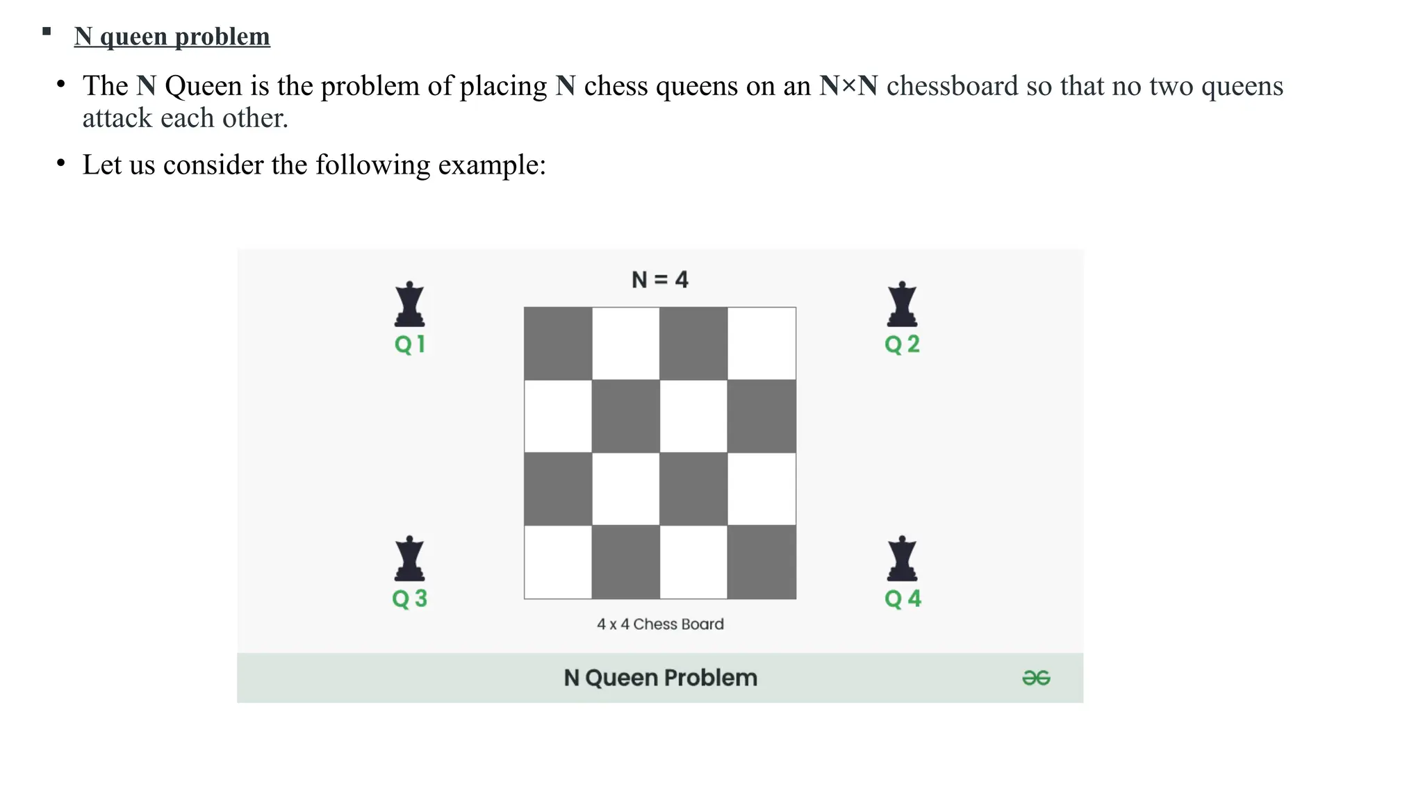
19.  N queen problem
• The N Queen is the problem of placing N chess queens on an N×N chessboard so that no two queens
attack each other.
• Let us consider the following example:

20. N Queen Problem using Backtracking:
Following steps to be used to solve the problem:
• Start in the leftmost column
• If all queens are placed return true
• Try all rows in the current column. Do the following for every row.
• If the queen can be placed safely in this row
• Then mark this [row, column] as part of the solution and recursively check if placing queen here
leads to a solution.
• If placing the queen in [row, column] leads to a solution then return true.
• If placing queen doesn’t lead to a solution then unmark this [row, column] then backtrack and try
other rows.
• If all rows have been tried and valid solution is not found return false to trigger backtracking.

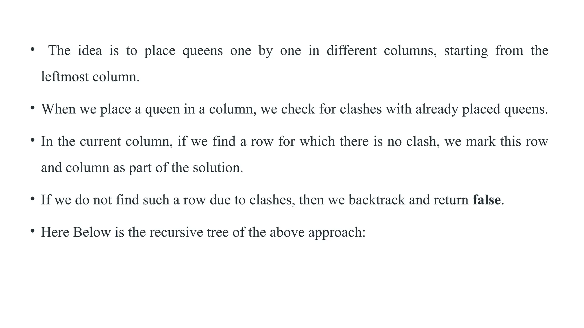
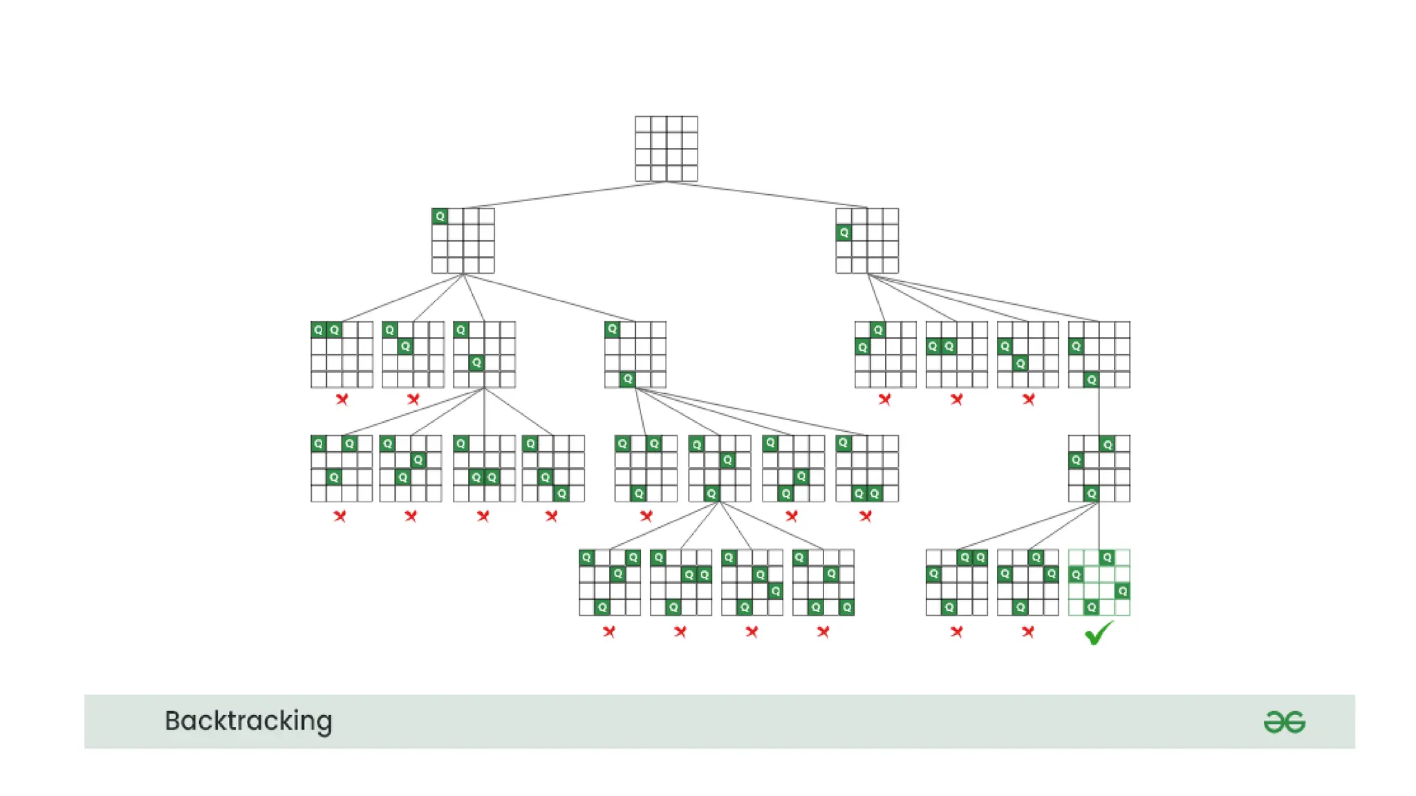
21. • The idea is to place queens one by one in different columns, starting from the
leftmost column.
• When we place a queen in a column, we check for clashes with already placed queens.
• In the current column, if we find a row for which there is no clash, we mark this row
and column as part of the solution.
• If we do not find such a row due to clashes, then we backtrack and return false.
• Here Below is the recursive tree of the above approach:

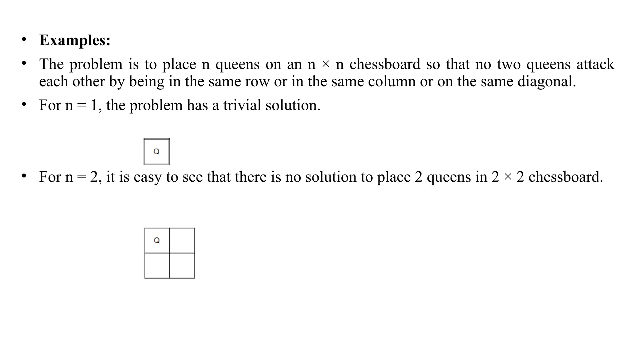
22. • Examples:
• The problem is to place n queens on an n × n chessboard so that no two queens attack
each other by being in the same row or in the same column or on the same diagonal.
• For n = 1, the problem has a trivial solution.
• For n = 2, it is easy to see that there is no solution to place 2 queens in 2 × 2 chessboard.

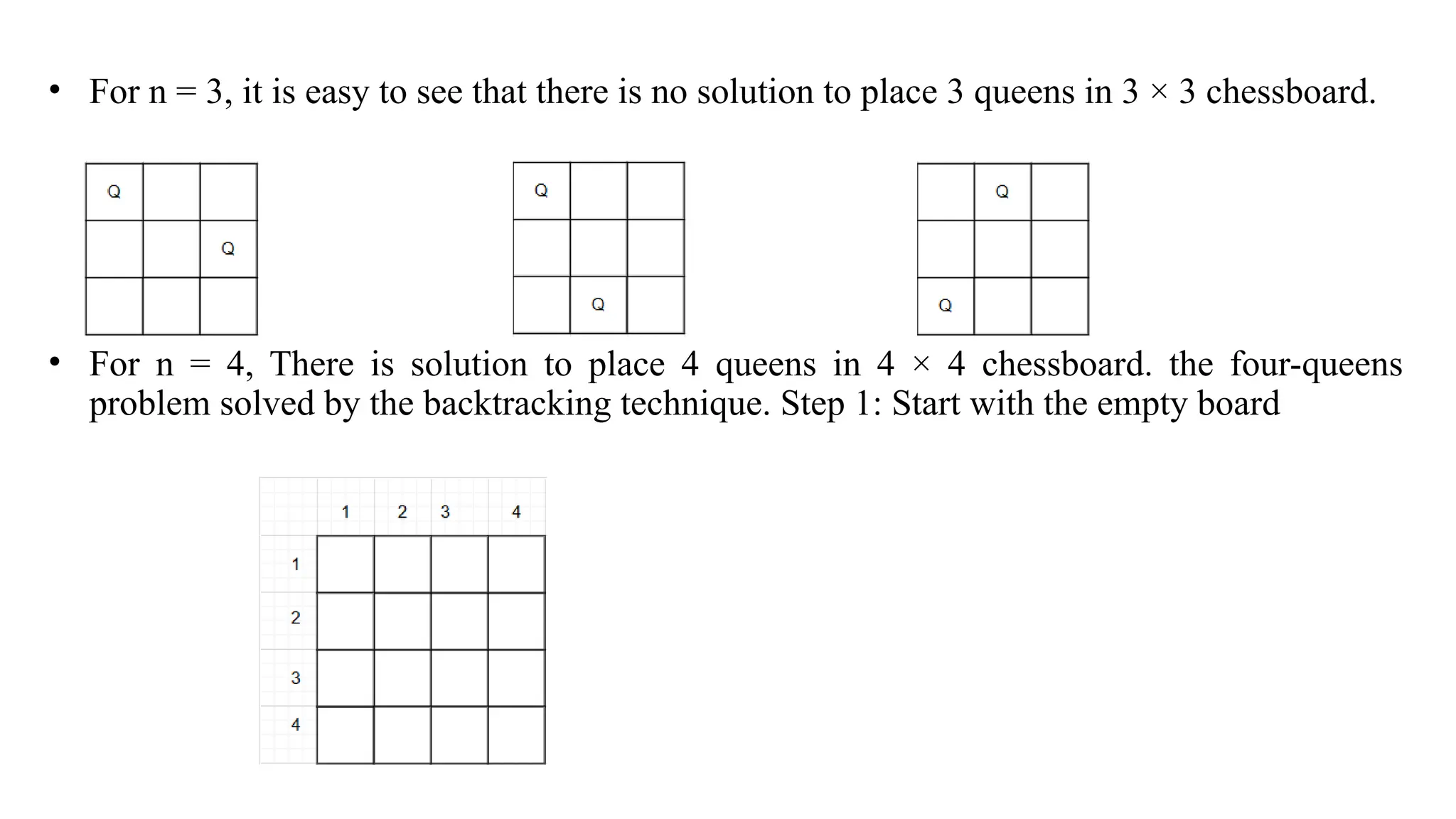
23. • For n = 3, it is easy to see that there is no solution to place 3 queens in 3 × 3 chessboard.
• For n = 4, There is solution to place 4 queens in 4 × 4 chessboard. the four-queens
problem solved by the backtracking technique. Step 1: Start with the empty board

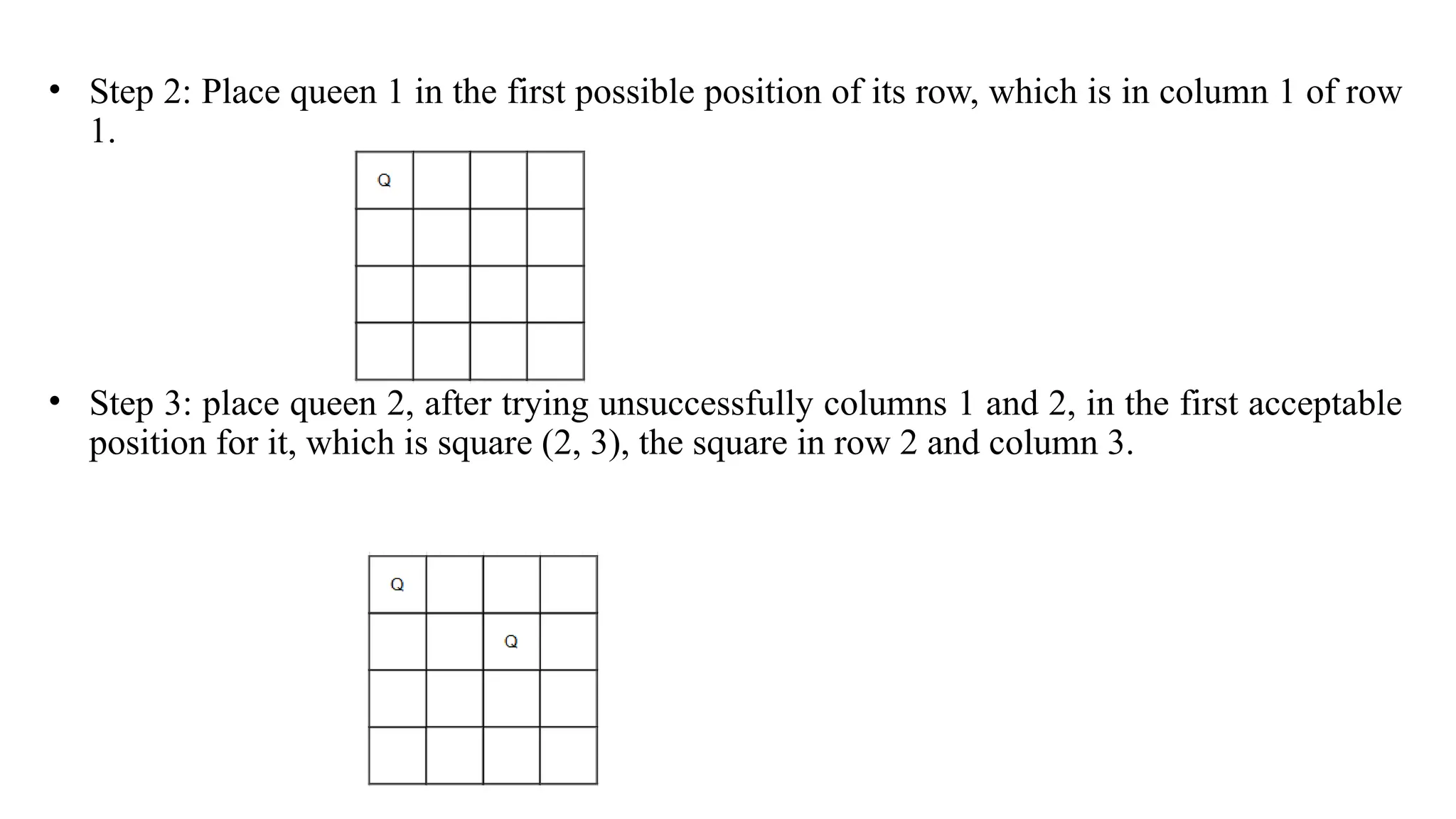
24. • Step 2: Place queen 1 in the first possible position of its row, which is in column 1 of row
1.
• Step 3: place queen 2, after trying unsuccessfully columns 1 and 2, in the first acceptable
position for it, which is square (2, 3), the square in row 2 and column 3.

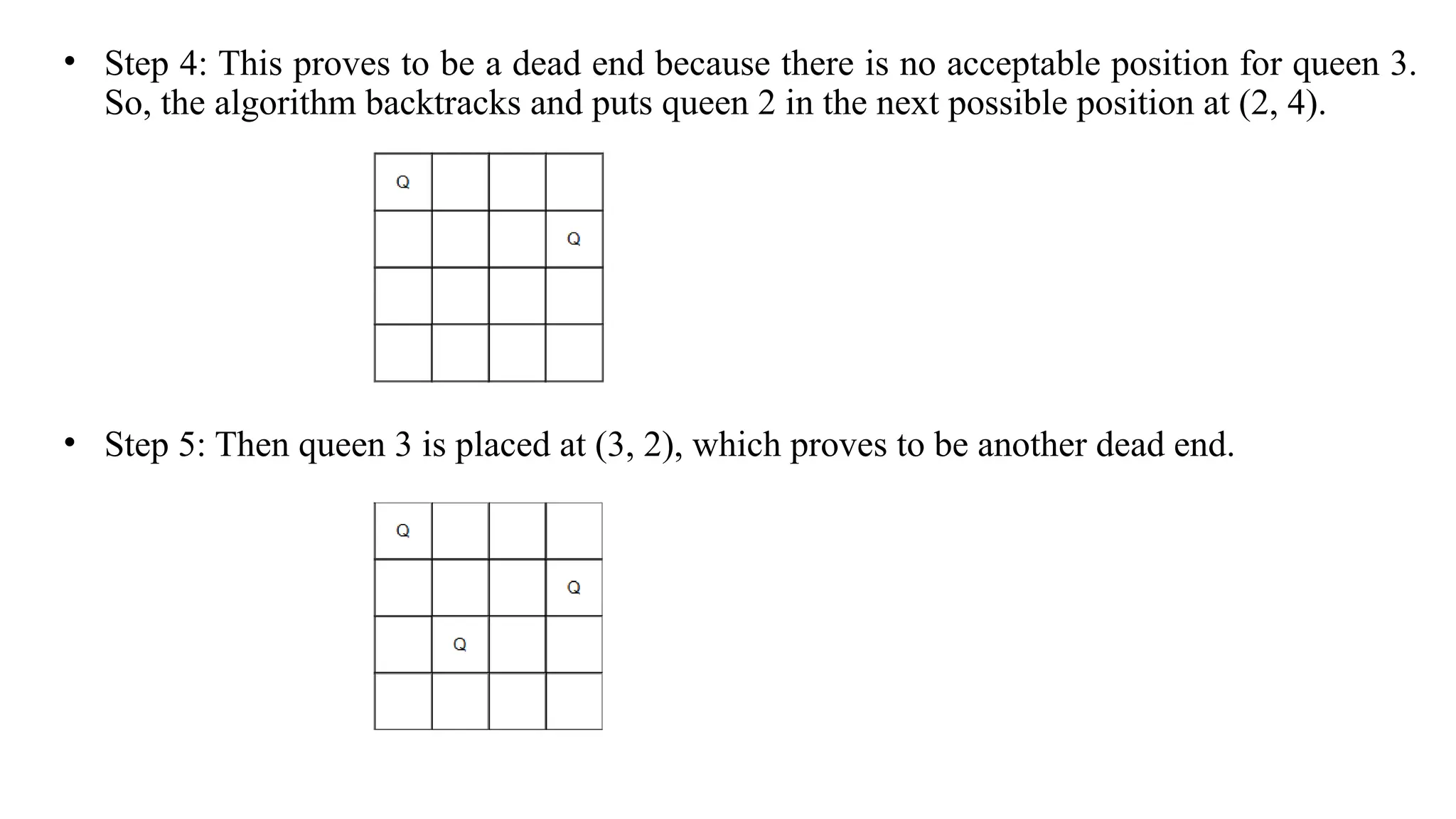
25. • Step 4: This proves to be a dead end because there is no acceptable position for queen 3.
So, the algorithm backtracks and puts queen 2 in the next possible position at (2, 4).
• Step 5: Then queen 3 is placed at (3, 2), which proves to be another dead end.

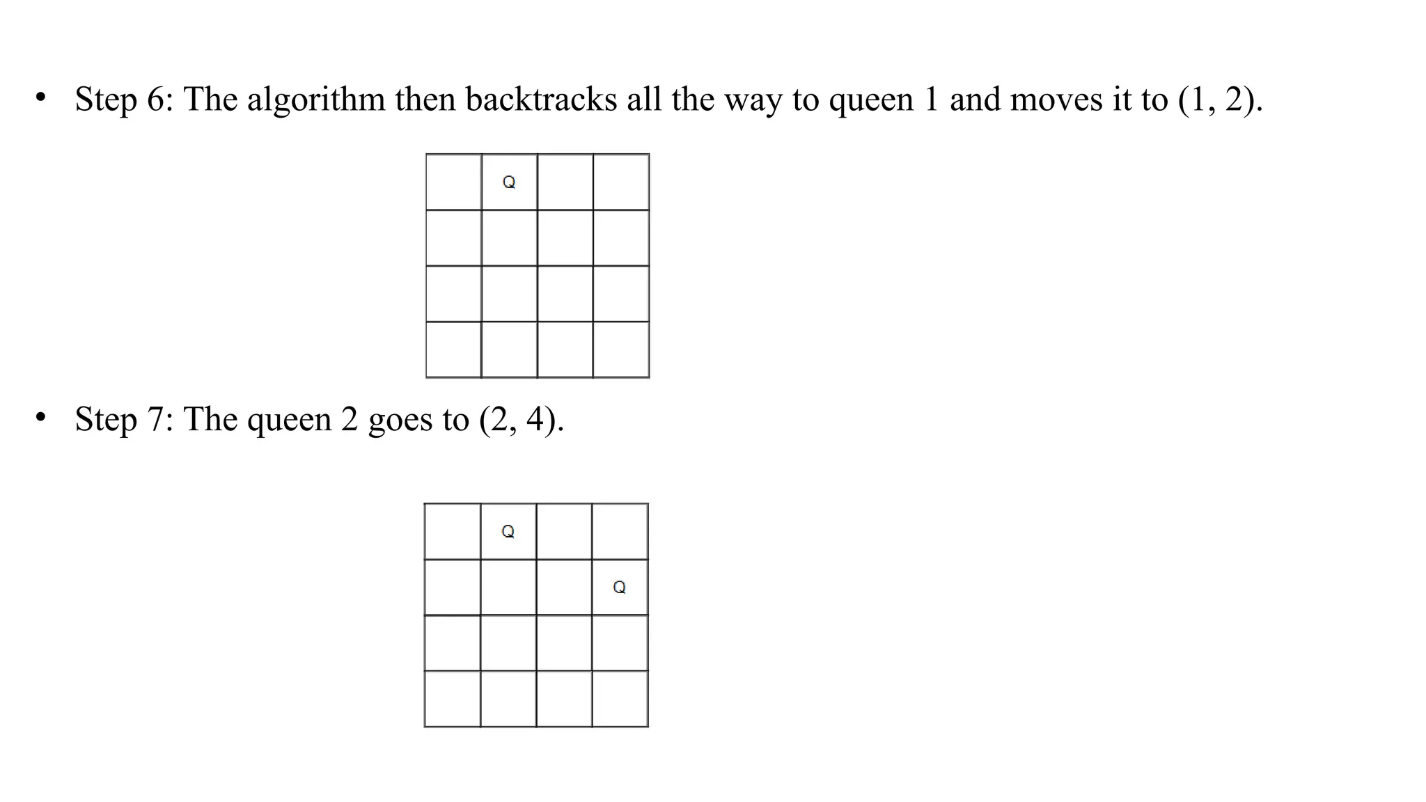
26. • Step 6: The algorithm then backtracks all the way to queen 1 and moves it to (1, 2).
• Step 7: The queen 2 goes to (2, 4).

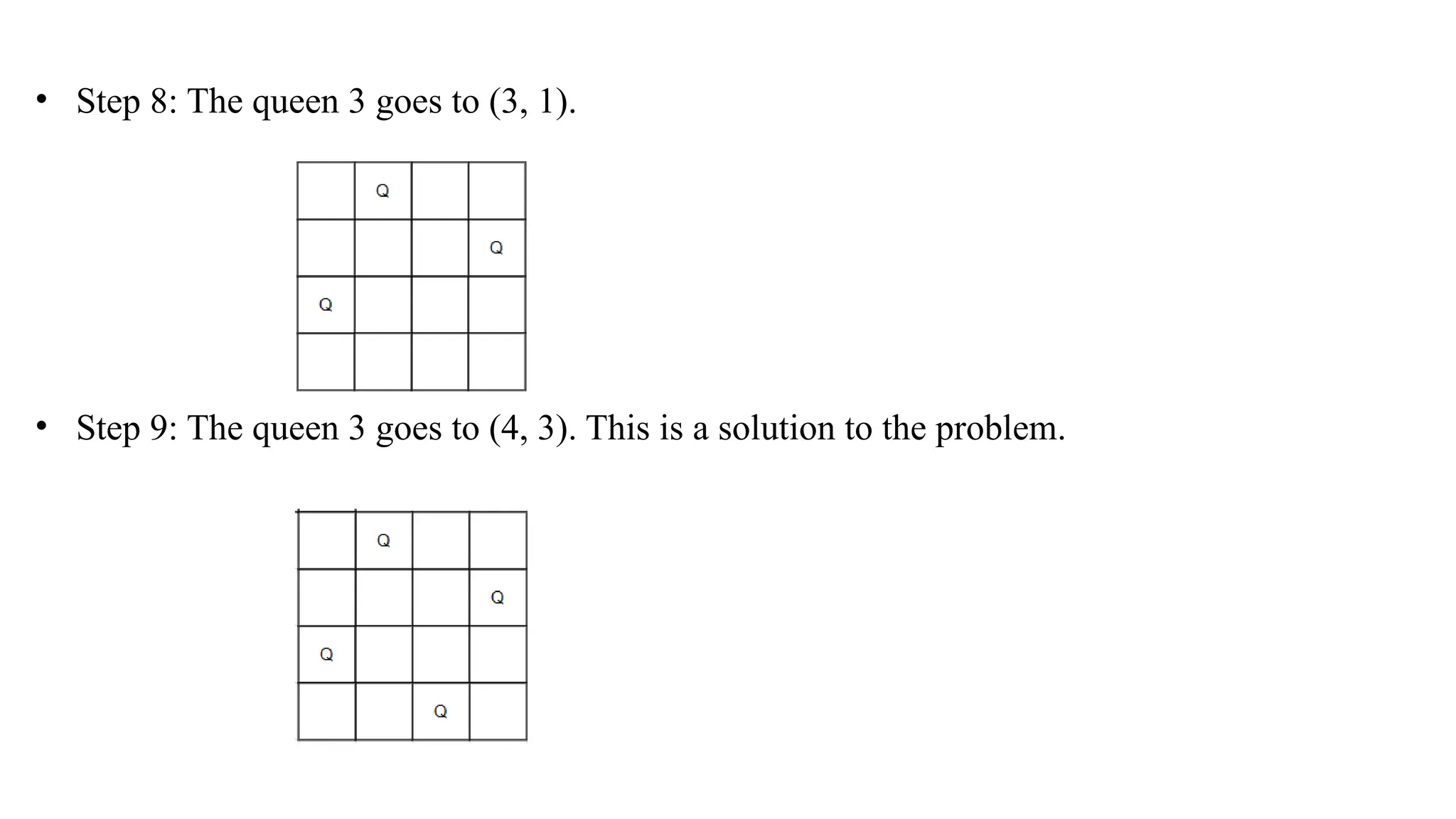
27. • Step 8: The queen 3 goes to (3, 1).
• Step 9: The queen 3 goes to (4, 3). This is a solution to the problem.

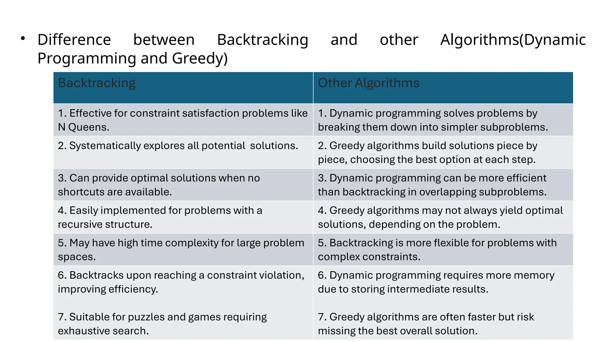
29. • Difference between Backtracking and other Algorithms(Dynamic
Programming and Greedy)
Backtracking Other Algorithms
1. Effective for constraint satisfaction problems like
N Queens.
1. Dynamic programming solves problems by
breaking them down into simpler subproblems.
2. Systematically explores all potential solutions. 2. Greedy algorithms build solutions piece by
piece, choosing the best option at each step.
3. Can provide optimal solutions when no
shortcuts are available.
3. Dynamic programming can be more efficient
than backtracking in overlapping subproblems.
4. Easily implemented for problems with a
recursive structure.
4. Greedy algorithms may not always yield optimal
solutions, depending on the problem.
5. May have high time complexity for large problem
spaces.
5. Backtracking is more flexible for problems with
complex constraints.
6. Backtracks upon reaching a constraint violation,
improving efficiency.
7. Suitable for puzzles and games requiring
exhaustive search.
6. Dynamic programming requires more memory
due to storing intermediate results.
7. Greedy algorithms are often faster but risk
missing the best overall solution.

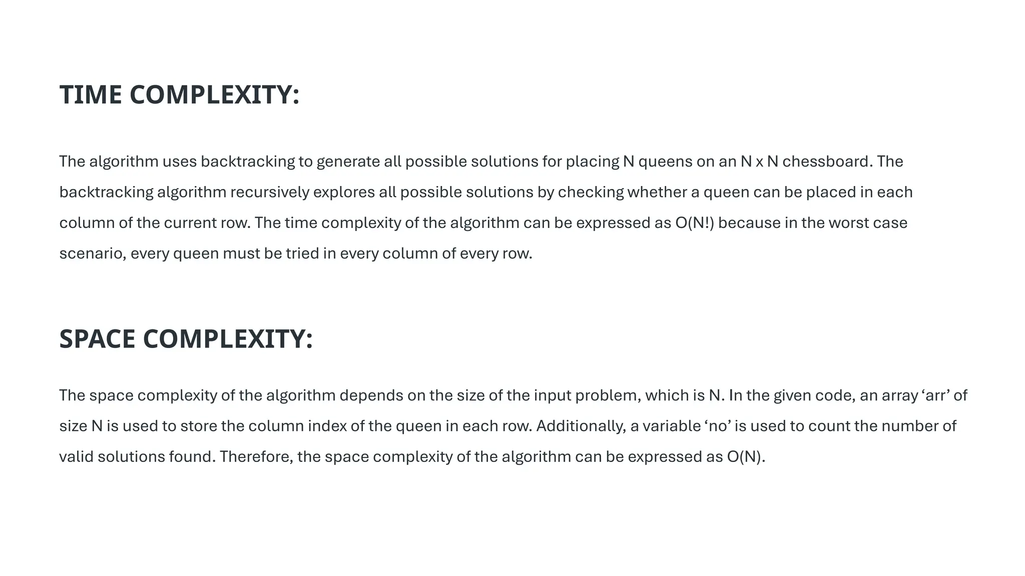
30. TIME COMPLEXITY:
The algorithm uses backtracking to generate all possible solutions for placing N queens on an N x N chessboard. The
backtracking algorithm recursively explores all possible solutions by checking whether a queen can be placed in each
column of the current row. The time complexity of the algorithm can be expressed as O(N!) because in the worst case
scenario, every queen must be tried in every column of every row.
SPACE COMPLEXITY:
The space complexity of the algorithm depends on the size of the input problem, which is N. In the given code, an array ‘arr’ of
size N is used to store the column index of the queen in each row. Additionally, a variable ‘no’ is used to count the number of
valid solutions found. Therefore, the space complexity of the algorithm can be expressed as O(N).

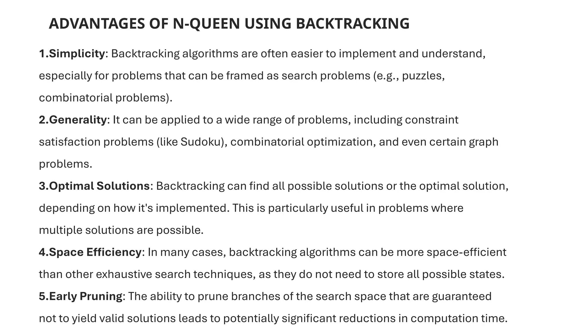
31. ADVANTAGES OF N-QUEEN USING BACKTRACKING
1.Simplicity: Backtracking algorithms are often easier to implement and understand,
especially for problems that can be framed as search problems (e.g., puzzles,
combinatorial problems).
2.Generality: It can be applied to a wide range of problems, including constraint
satisfaction problems (like Sudoku), combinatorial optimization, and even certain graph
problems.
3.Optimal Solutions: Backtracking can find all possible solutions or the optimal solution,
depending on how it's implemented. This is particularly useful in problems where
multiple solutions are possible.
4.Space Efficiency: In many cases, backtracking algorithms can be more space-efficient
than other exhaustive search techniques, as they do not need to store all possible states.
5.Early Pruning: The ability to prune branches of the search space that are guaranteed
not to yield valid solutions leads to potentially significant reductions in computation time.

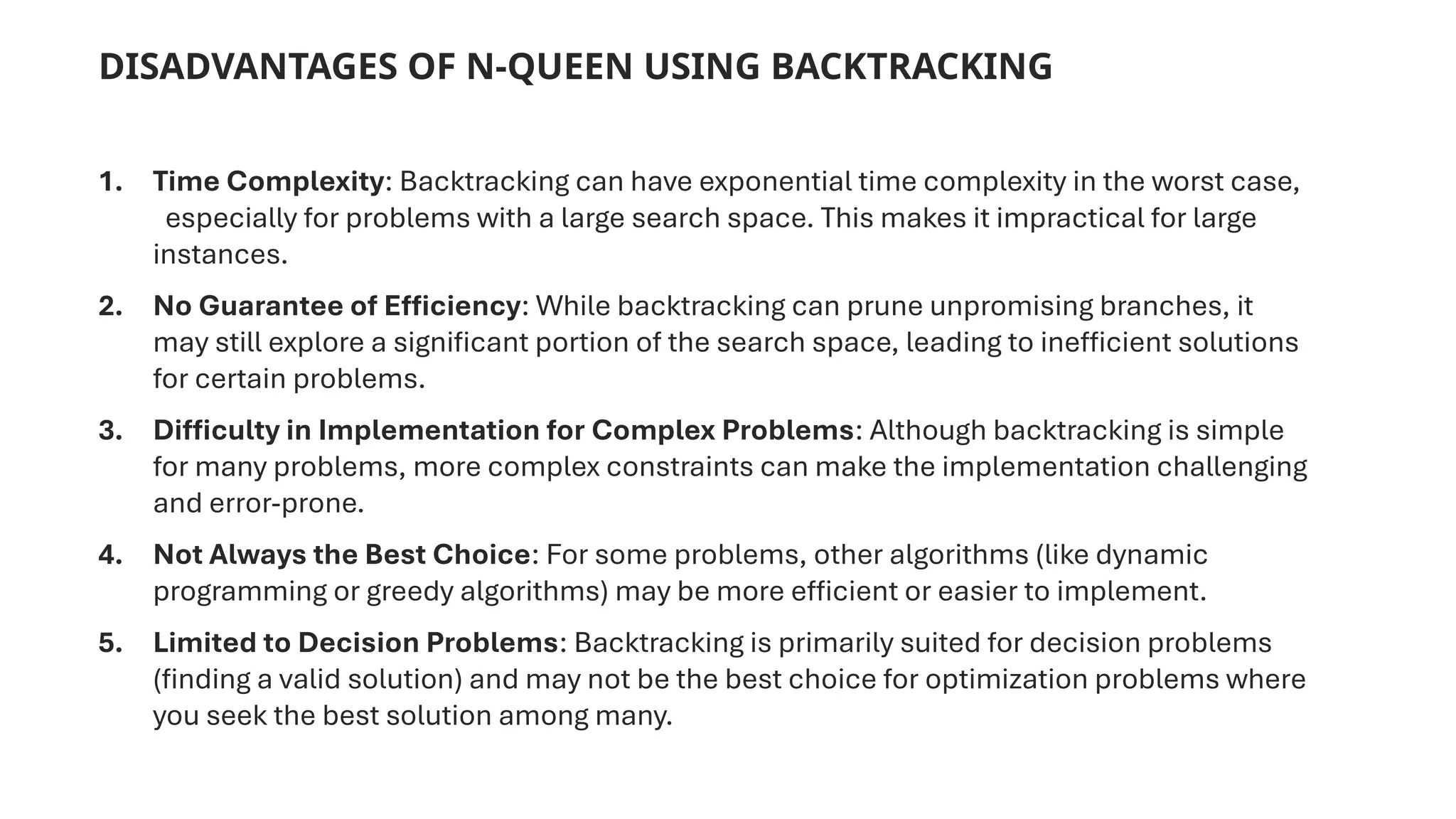
32. DISADVANTAGES OF N-QUEEN USING BACKTRACKING
1. Time Complexity: Backtracking can have exponential time complexity in the worst case,
especially for problems with a large search space. This makes it impractical for large
instances.
2. No Guarantee of Efficiency: While backtracking can prune unpromising branches, it
may still explore a significant portion of the search space, leading to inefficient solutions
for certain problems.
3. Difficulty in Implementation for Complex Problems: Although backtracking is simple
for many problems, more complex constraints can make the implementation challenging
and error-prone.
4. Not Always the Best Choice: For some problems, other algorithms (like dynamic
programming or greedy algorithms) may be more efficient or easier to implement.
5. Limited to Decision Problems: Backtracking is primarily suited for decision problems
(finding a valid solution) and may not be the best choice for optimization problems where
you seek the best solution among many.

33. APPLICATIONS :
1. Timetable Scheduling: Assigning exams, meetings, or events to times and rooms without conflicts,
ensuring no overlap in resources.
2. Processor Allocation: Optimizing task assignments to processors in parallel computing to avoid
resource conflicts.
3. Frequency Assignment: Allocating frequencies to radio towers or communication devices to
prevent interference.
4. Sensor Placement: Positioning sensors in a monitoring field to maximize coverage without
overlapping signals.
5. Puzzle Solving: Used in solving other constraint-based puzzles like Sudoku, where elements must
meet specific non-conflicting conditions.

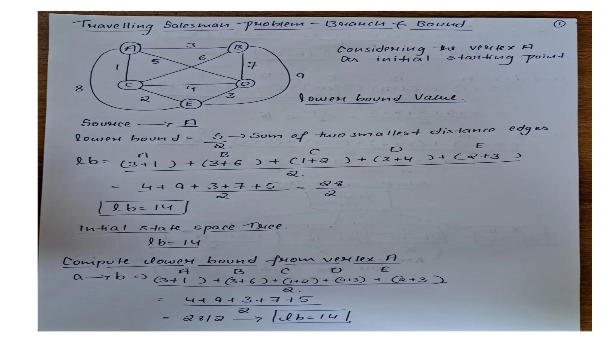
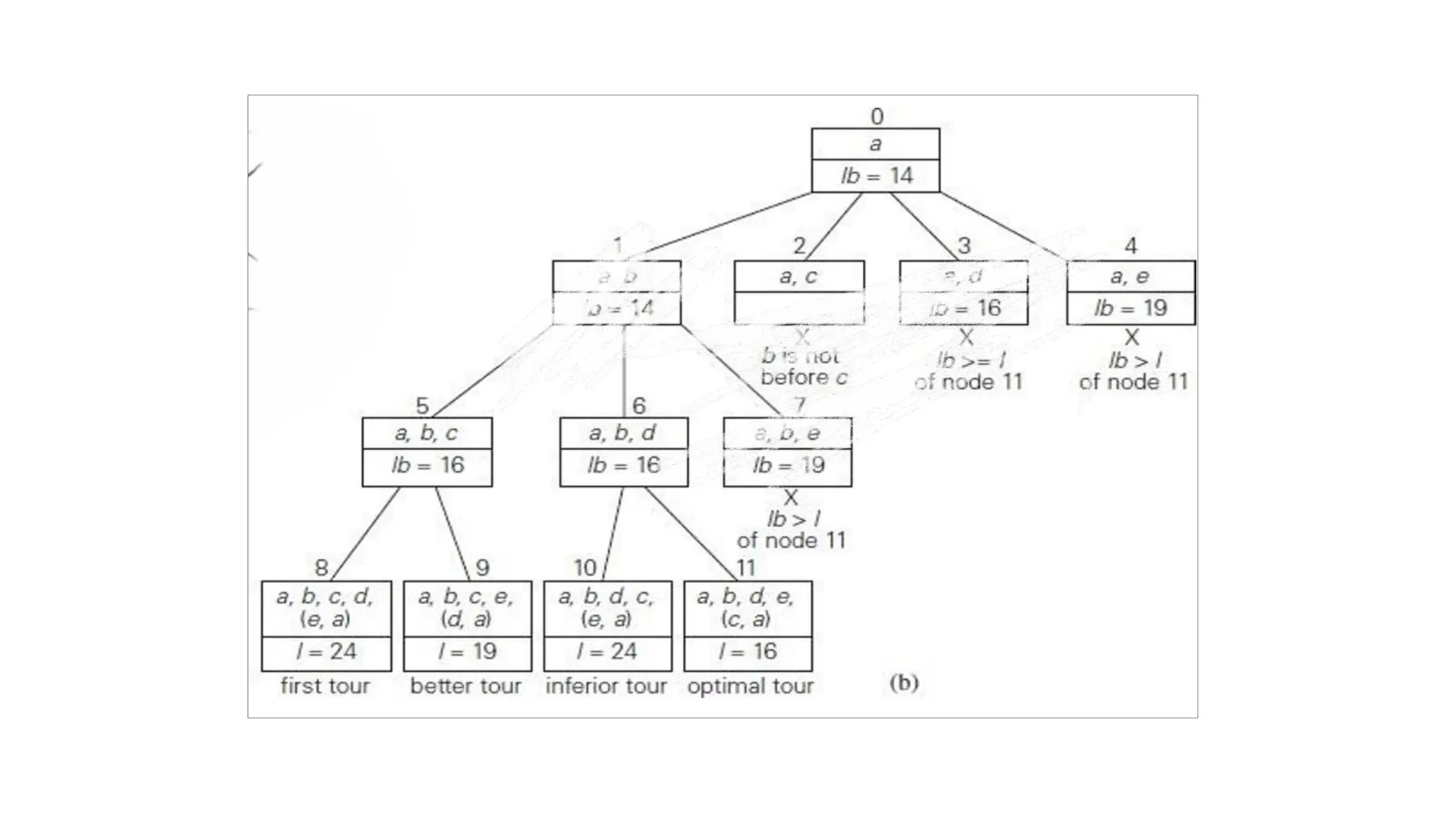
34. TRAVELLING SALESMAN PROBLEM
Problem
Given n cities, a salesman starts at a specified city(often
called source) visit all n-1 cities only once and 0 return to
the city from where he has started
Travelling Salesman Problem
using
Branch & Bound Technique
using
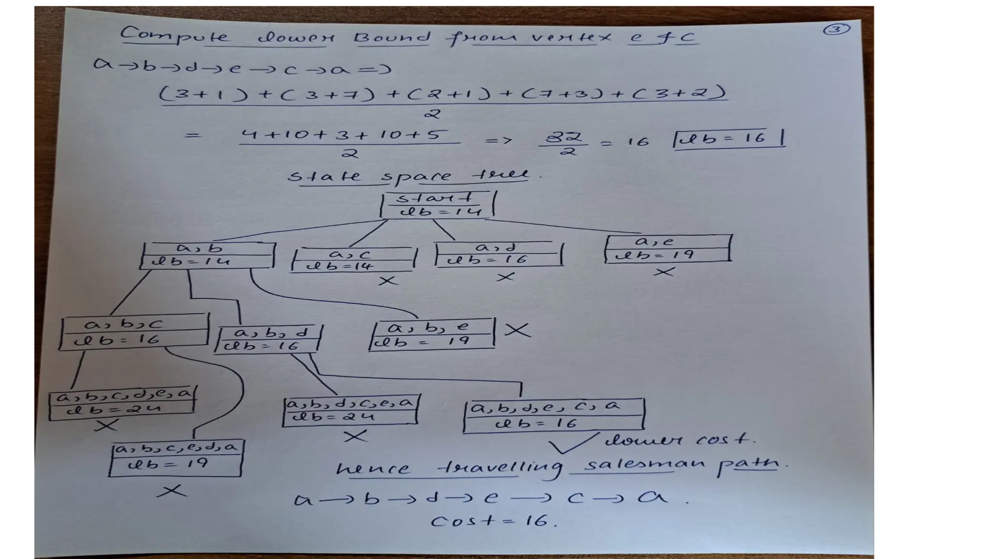
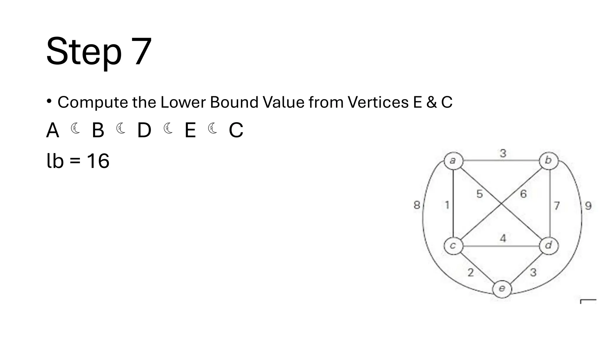
LOWER BOUND FORMULA

35. TRAVELLING SALESMAN PROBLEM
Objective
Find a route through the cities that minimize the cost thereby
maximize the profit
Model
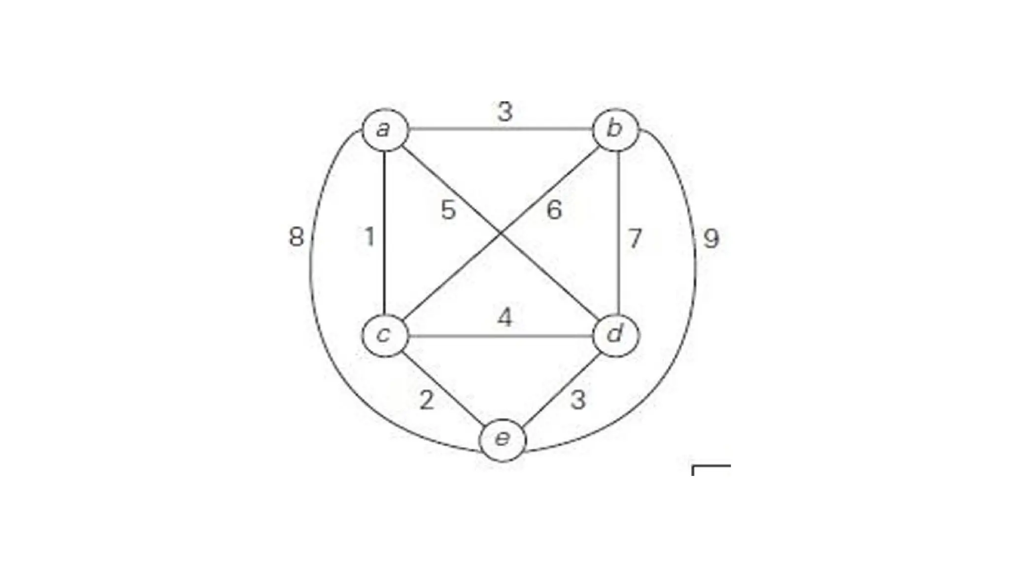
• The vertices of the graphs represent the various cities
• The weights associated with edges represent the distances
between two cities or the cost involved from one city to other city
during travelling

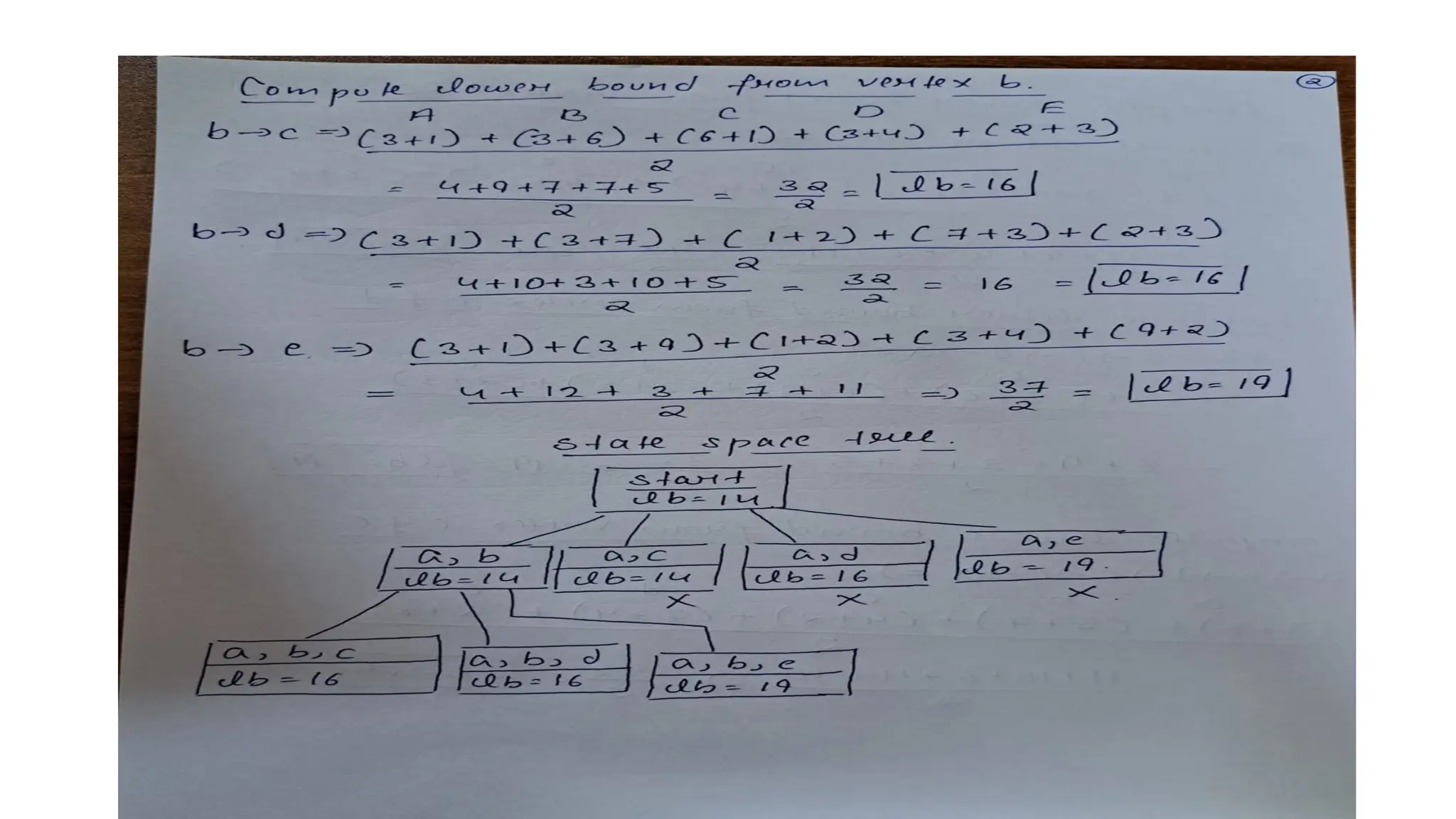
36. TRAVELLING SALESMAN PROBLEM
Observations in Constructing State
Space Tree
• Tour always starts at A (any Source Node)
• In the tour the first and last city remains same whereas other
intermediate nodes be distinct
• Visit Node B before Node C

38. Formula to Compute Lower Bound Value
Lower Bound =
lb =

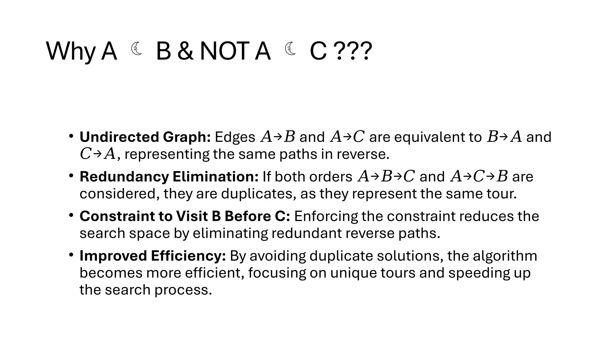
39. Why A  B & NOT A  C ???
• Undirected Graph: Edges → and → are equivalent to → and
𝐴 𝐵 𝐴 𝐶 𝐵 𝐴
→ , representing the same paths in reverse.
𝐶 𝐴
• Redundancy Elimination: If both orders → → and → → are
𝐴 𝐵 𝐶 𝐴 𝐶 𝐵
considered, they are duplicates, as they represent the same tour.
• Constraint to Visit B Before C: Enforcing the constraint reduces the
search space by eliminating redundant reverse paths.
• Improved Efficiency: By avoiding duplicate solutions, the algorithm
becomes more efficient, focusing on unique tours and speeding up
the search process.

40. Step 1
• Compute the General Lower Bound Value
lb =
lb =
lb = 14

44. Step 2
• Compute the Lower Bound Value from Vertex A
A  B lb = 14
A  C lb = 14
A  D lb = 16 (approx.)
A  E lb = 19

46. Step 3
• Compute the Lower Bound Value from Vertex B
A  B  C lb = 16
A  B  D lb = 16
A  B  E lb = 19 (approx.)

49. Step 4
• Compute the Lower Bound Value from Vertices D & E
A  B  C  D  E
lb = 24

52. Step 5
• Compute the Lower Bound Value from Vertices D & E
A  B  C  E  D
lb = 19

54. Step 6
• Compute the Lower Bound Value from Vertices C & E
A  B  D  C  E
lb = 24

57. Step 7
• Compute the Lower Bound Value from Vertices E & C
A  B  D  E  C
lb = 16

59. Final Step
• The Optimal Path and its Lower Bound Value:
A  B  D  E  C
lb = 16

60. Algorithm
STEP 1:
Input
Distance matrix (symmetric), number of cities .
𝐷 𝑛

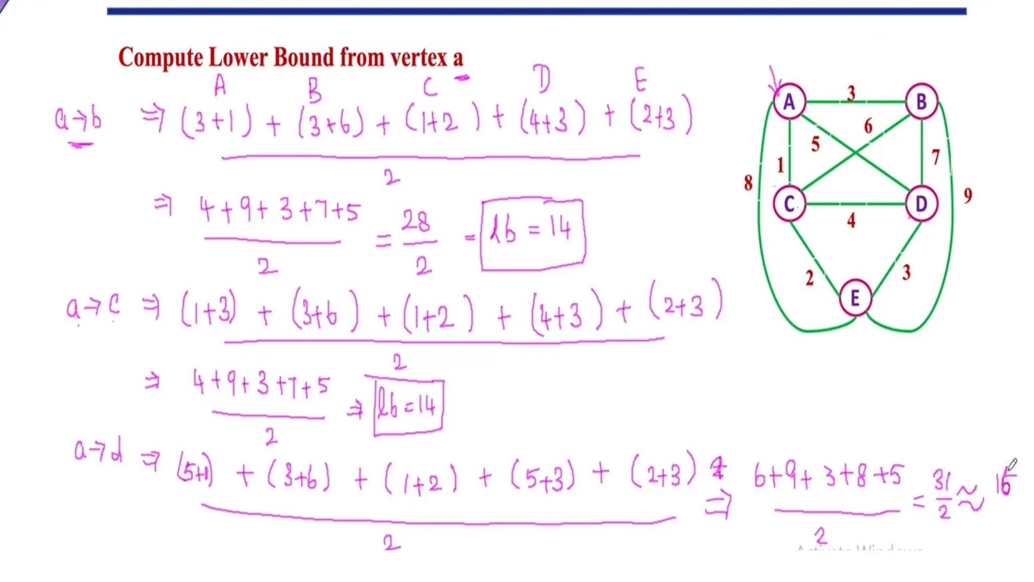
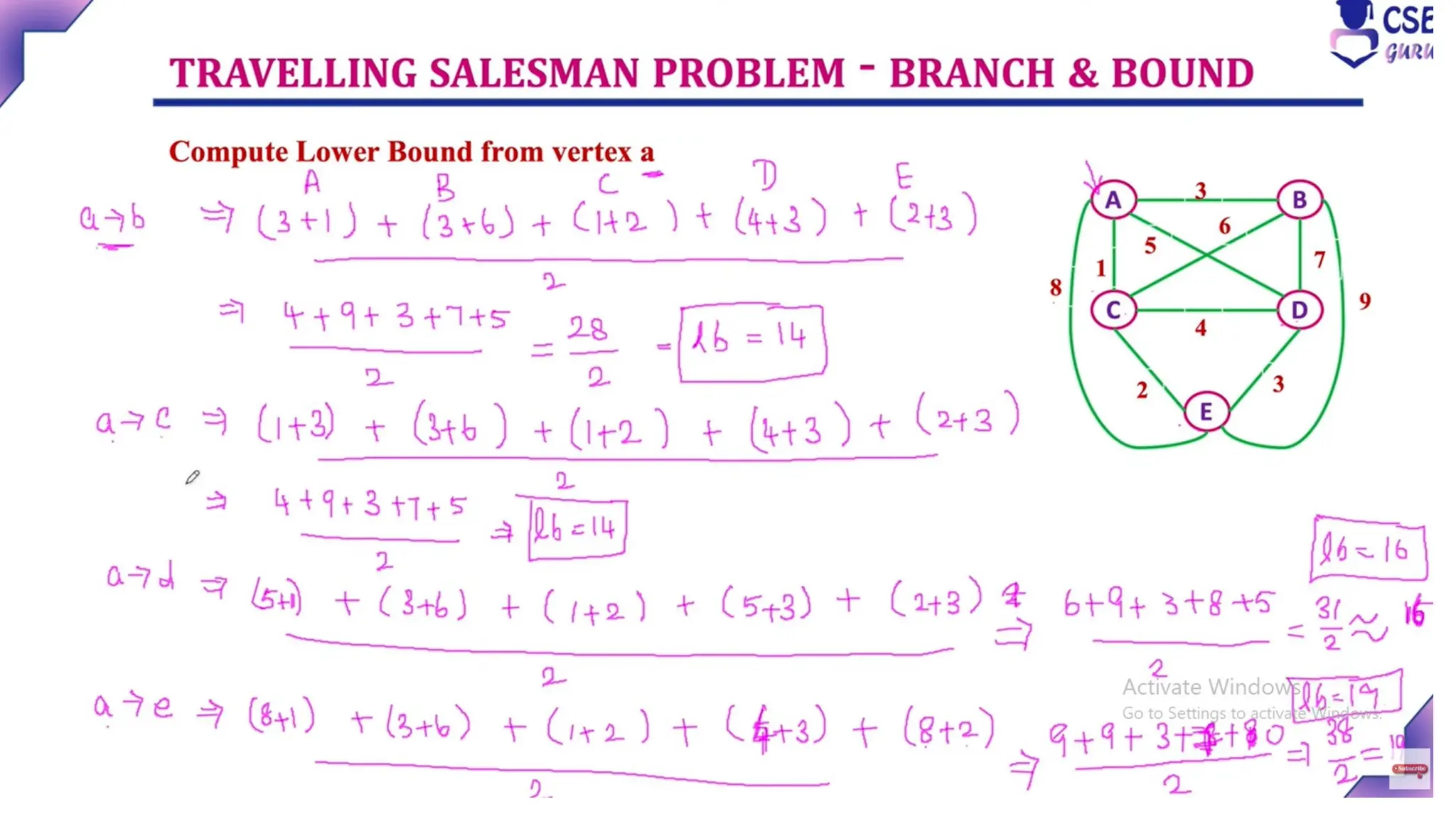
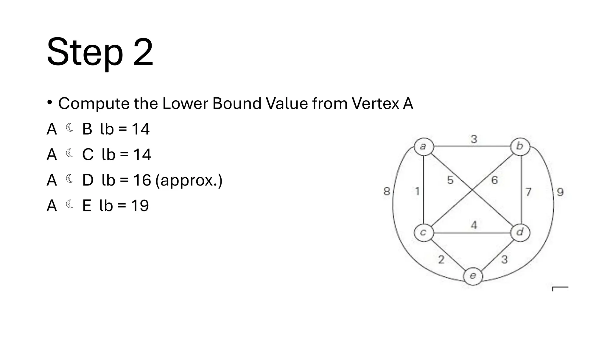
61. Algorithm
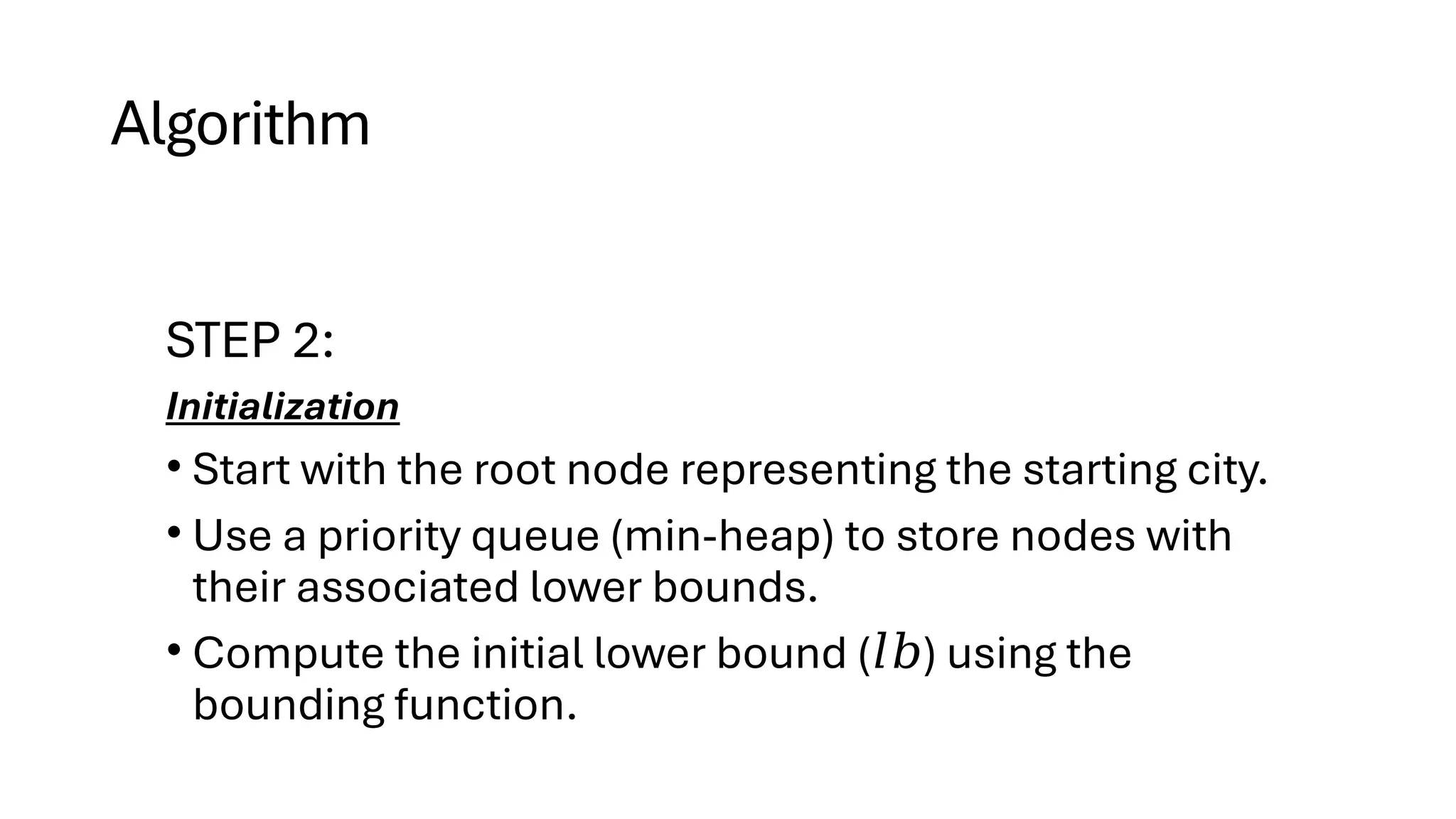
STEP 2:
Initialization
• Start with the root node representing the starting city.
• Use a priority queue (min-heap) to store nodes with
their associated lower bounds.
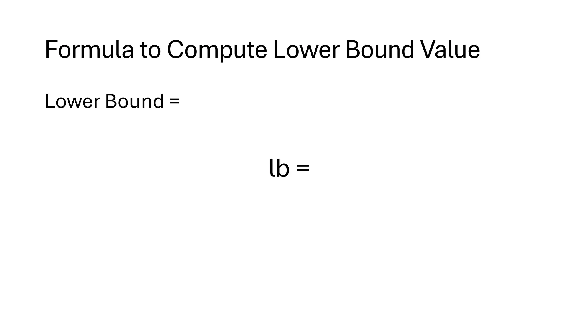
• Compute the initial lower bound ( ) using the
𝑙𝑏
bounding function.

62. Algorithm
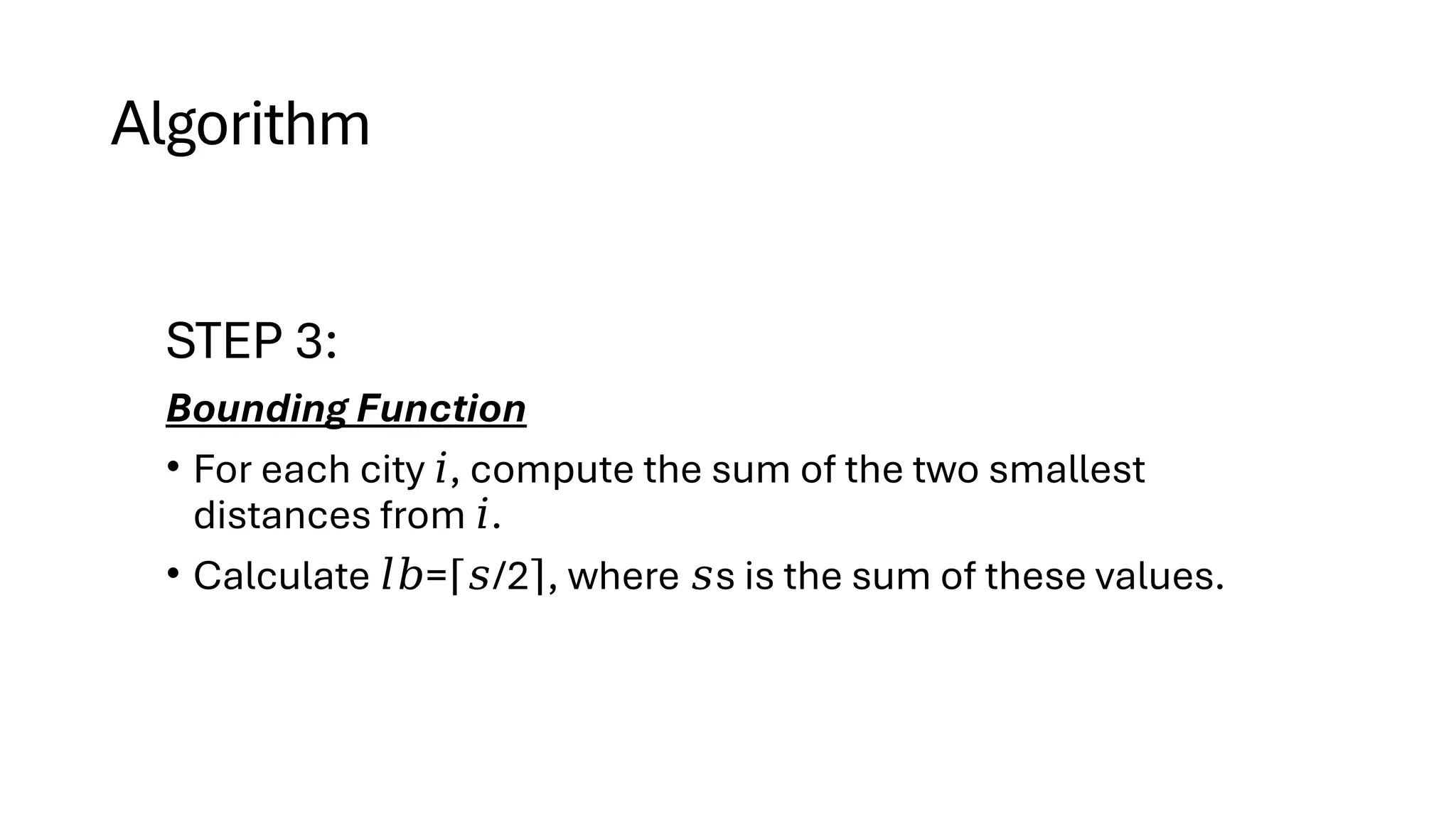
STEP 3:
Bounding Function
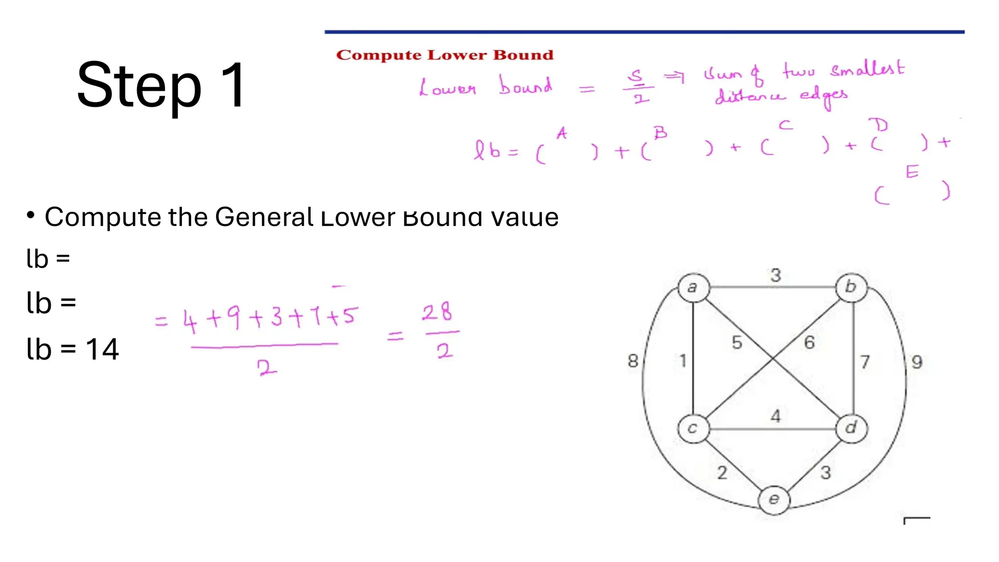
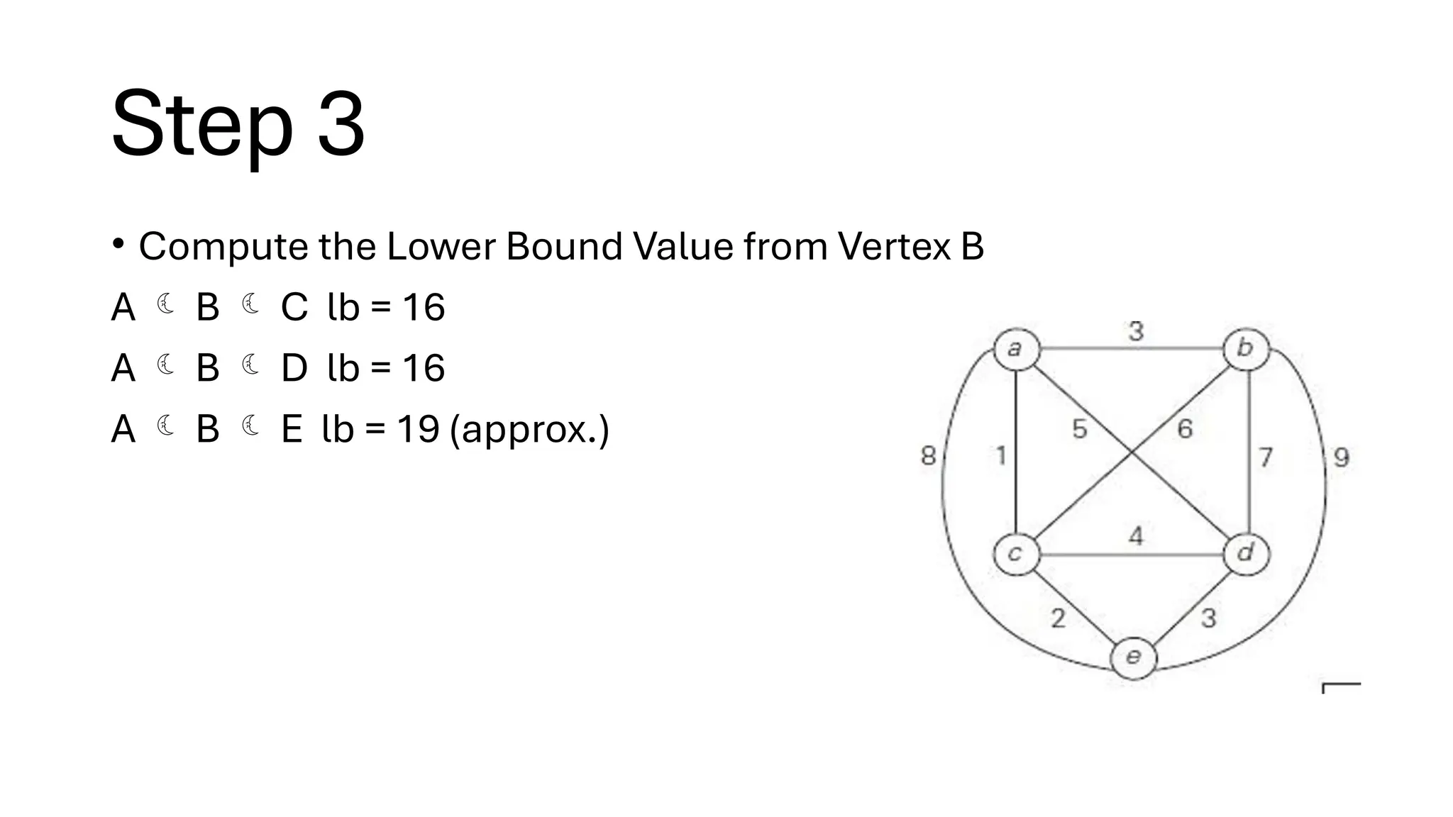
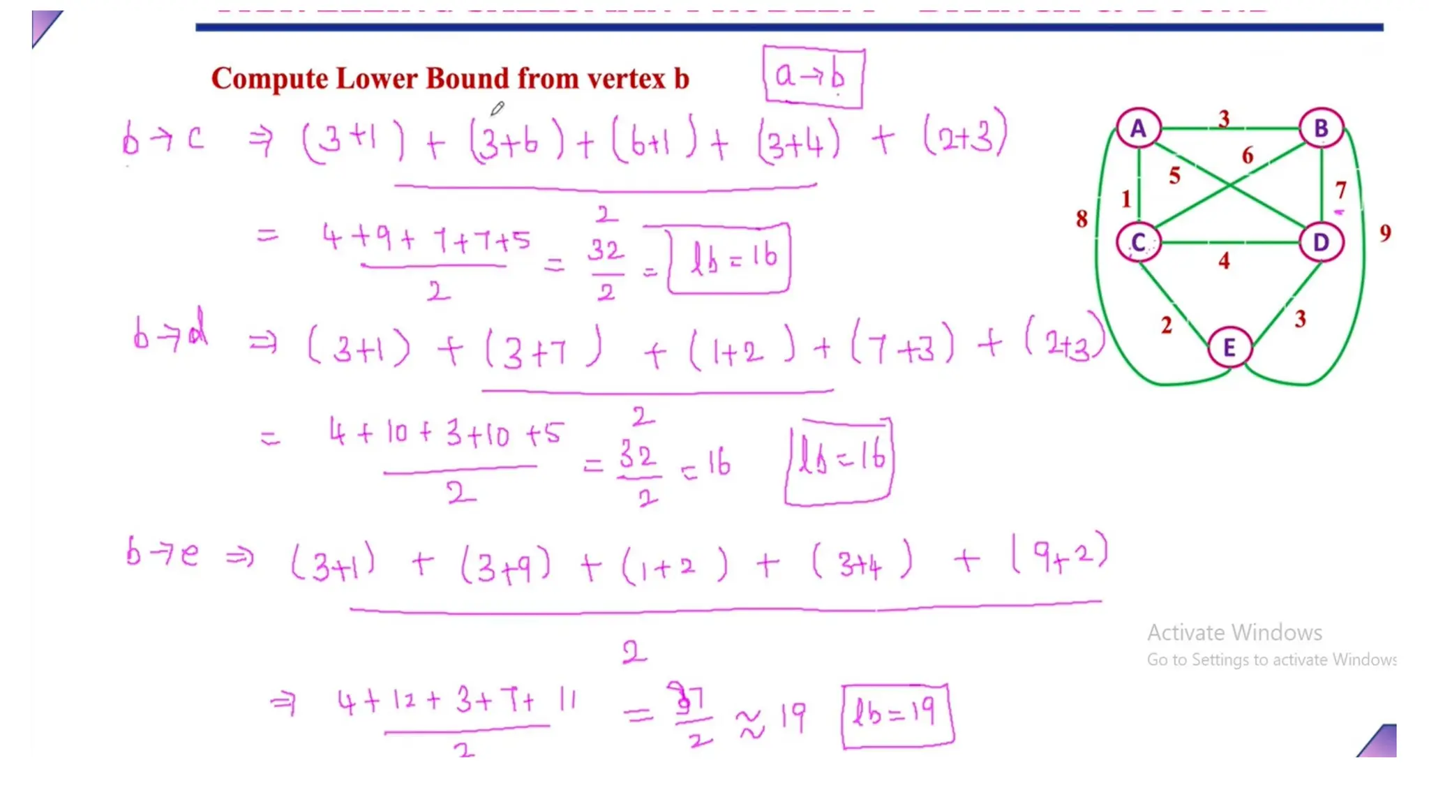
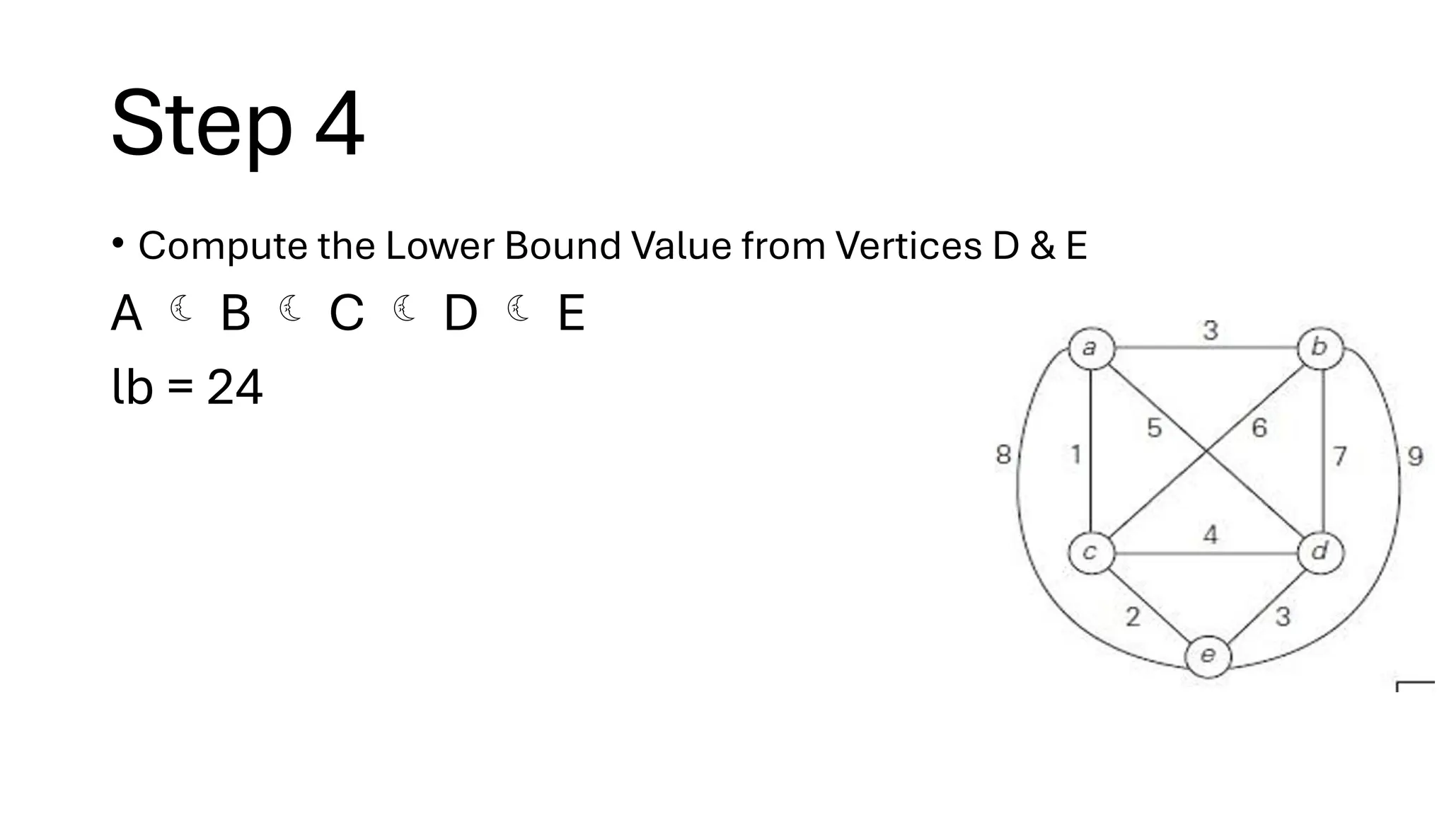
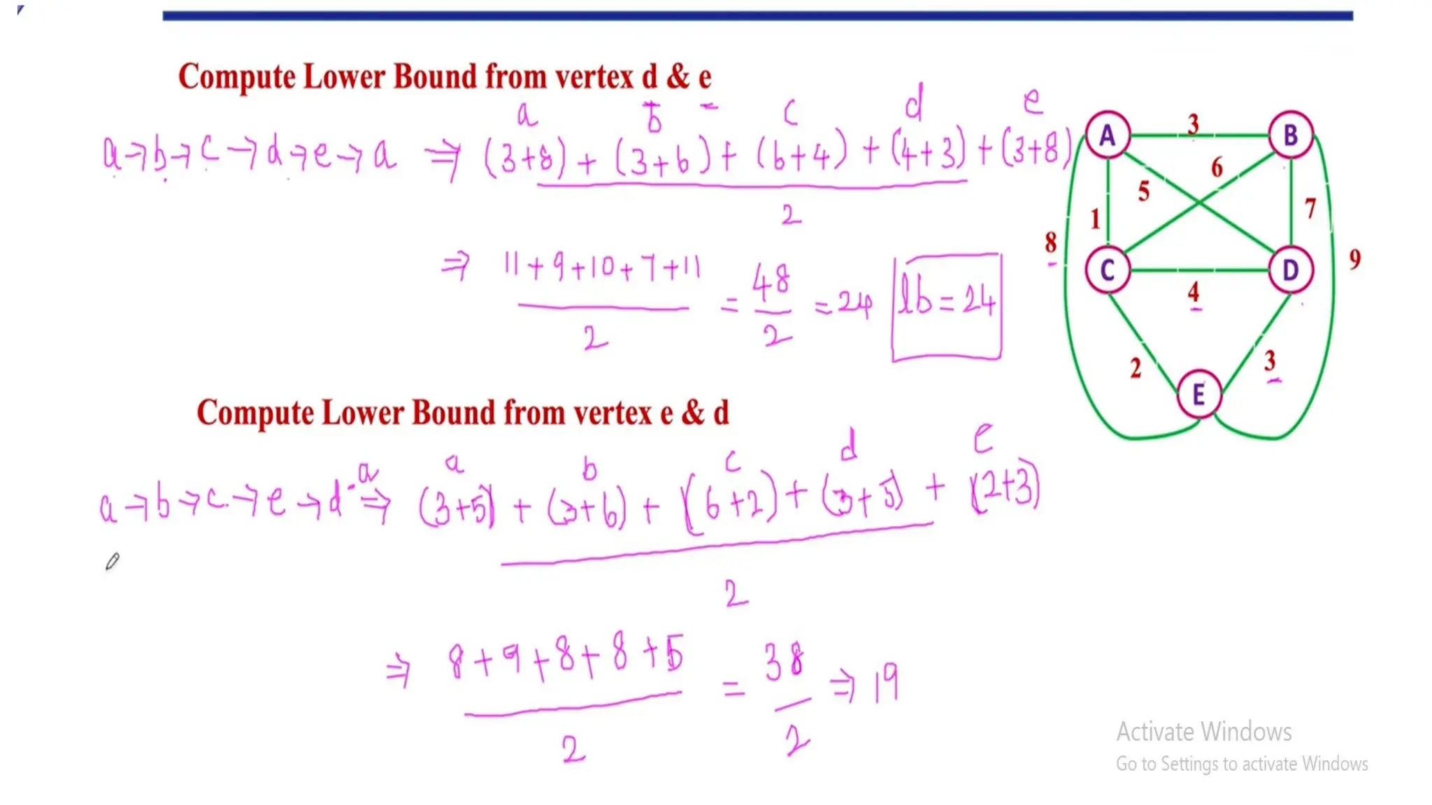
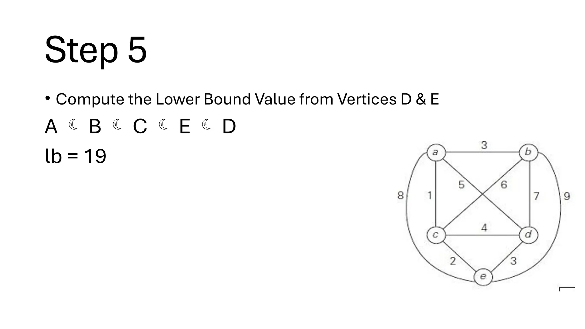
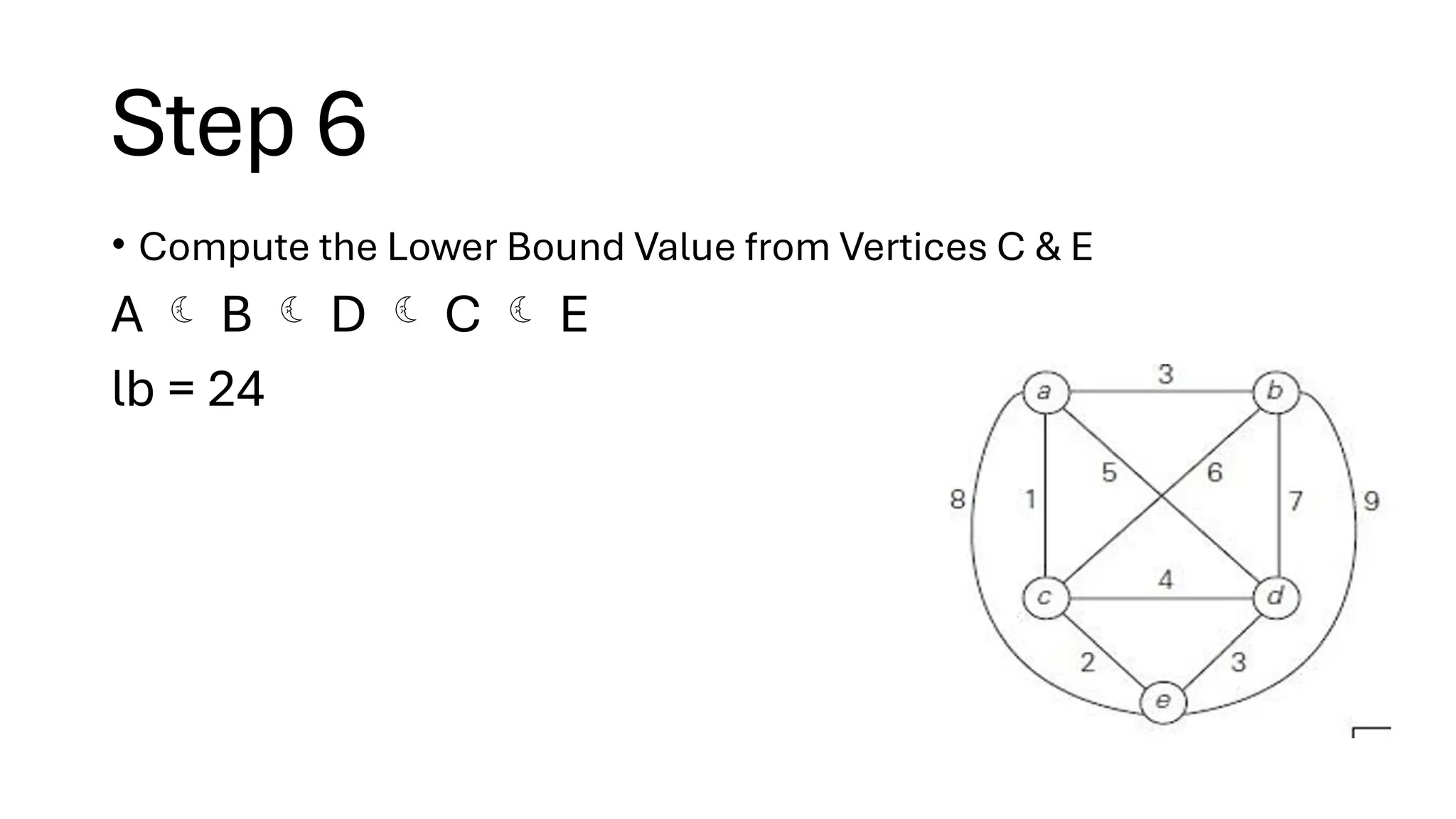
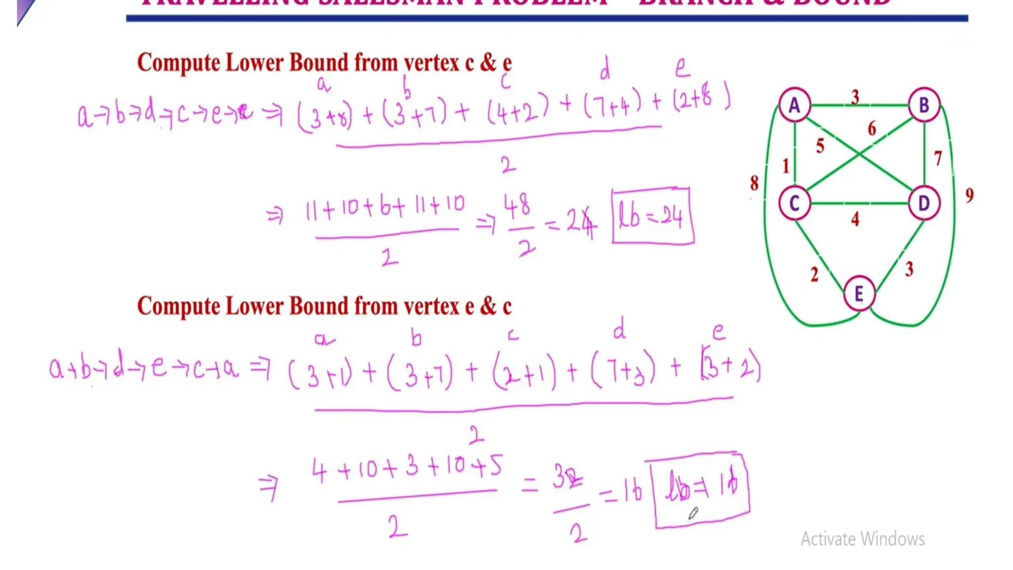
• For each city , compute the sum of the two smallest
𝑖
distances from .
𝑖
• Calculate = /2 , where s is the sum of these values.
𝑙𝑏 ⌈𝑠 ⌉ 𝑠

63. Algorithm
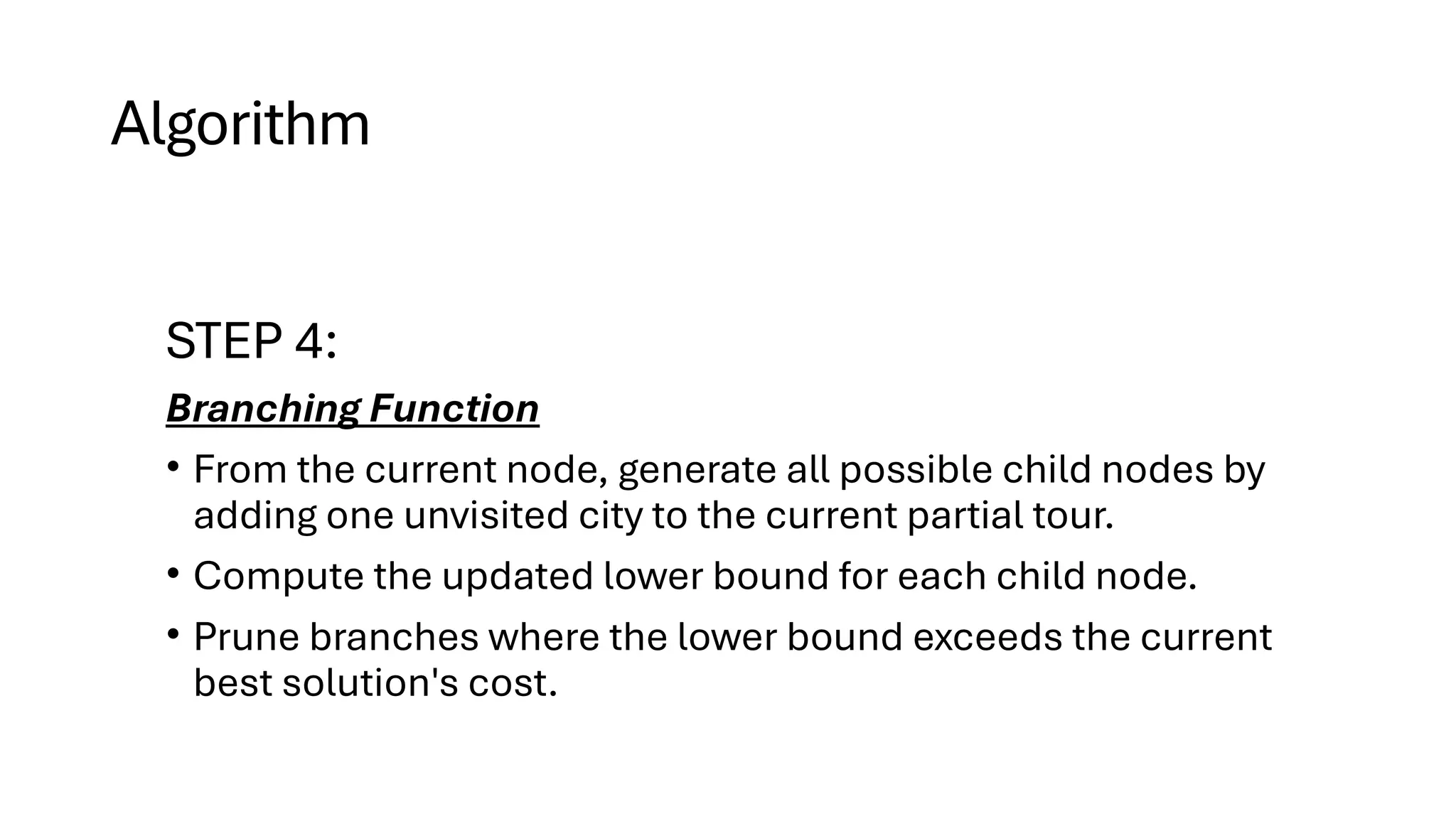
STEP 4:
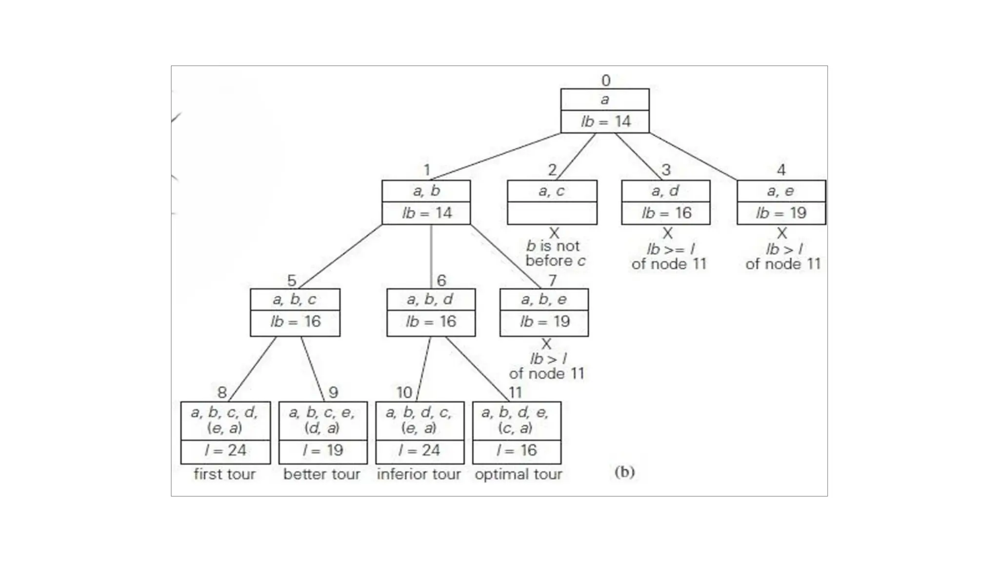
Branching Function
• From the current node, generate all possible child nodes by
adding one unvisited city to the current partial tour.
• Compute the updated lower bound for each child node.
• Prune branches where the lower bound exceeds the current
best solution's cost.

64. Algorithm
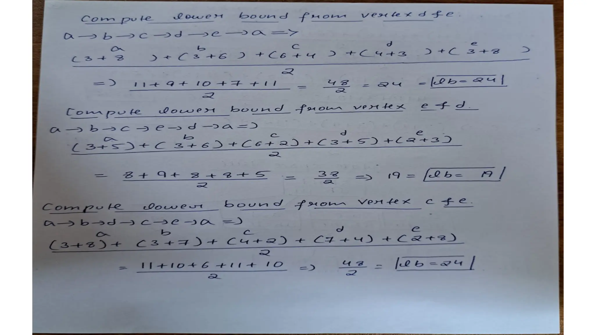
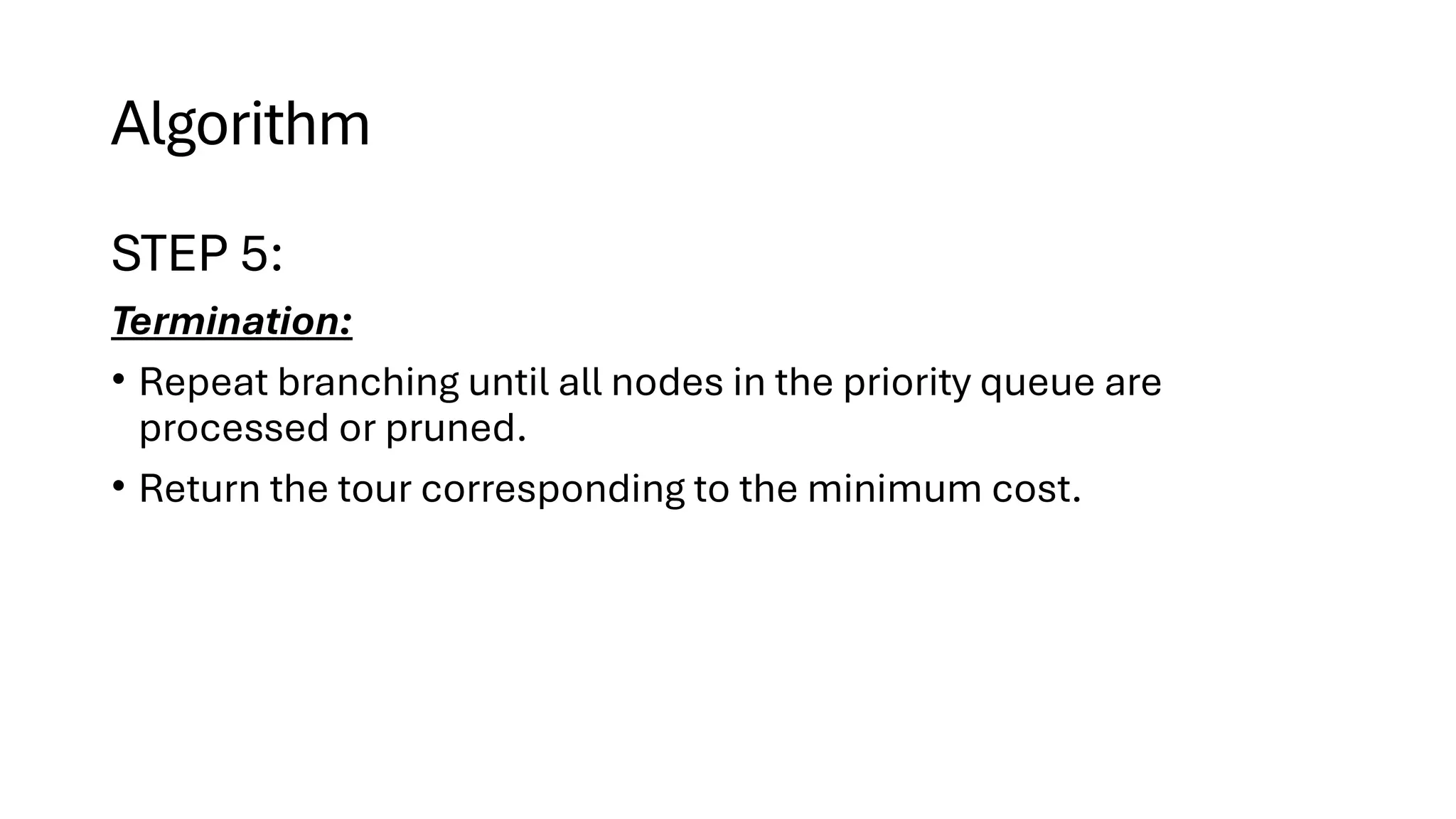
STEP 5:
Termination:
• Repeat branching until all nodes in the priority queue are
processed or pruned.
• Return the tour corresponding to the minimum cost.

65. Pseudocode for Bounding Function
function computeLowerBound(D, n):
s = 0
for each city i from 0 to n-1:
# Find the two smallest distances from city i
smallestDistances = findTwoSmallest(D[i])
s += sum(smallestDistances)
# Return the lower bound as ceil(s / 2)
return ceil(s / 2)

66. Pseudocode for Branching Function
function generateBranches(currentNode,
D, n, bestCost):
branches = [] # To store valid child nodes
for each city nextCity from 0 to n-1:
if nextCity is not in currentNode.path:
# Create new path by adding the next
city
newPath = currentNode.path +
[nextCity]
# Calculate the cost of the new path
newCost = currentNode.cost +
D[currentNode.path[-1]][nextCity]
# Compute the lower bound for the
new path
newBound = computeBound(D, n,
newPath, newCost)
# Only keep branches with bound <
bestCost
if newBound < bestCost:
childNode =
createNode(path=newPath,
cost=newCost, bound=newBound)
branches.append(childNode)
return branches

67. Time Complexity
Technique Time Complexity
Branch & Bound 𝑂( !) (worst case)
𝑛

73. Branch and Bound Algorithm-ASSIGNMENT PROBLEM
The Branch and Bound Algorithm is a method used
in combinatorial optimization problems to
systematically search for the best solution. It works by
dividing the problem into smaller subproblems, or
branches, and then eliminating certain branches based
on bounds on the optimal solution. This process
continues until the best solution is found or all branches
have been explored. Branch and Bound is commonly
used in problems like the traveling salesman and job
scheduling.

74. JAssignment Problem using Branch And Bound
Let there be N workers and N jobs. Any worker can be
assigned to perform any job, incurring some cost that
may vary depending on the work-job assignment. It is
required to perform all jobs by assigning exactly one
worker to each job and exactly one job to each agent in
such a way that the total cost of the assignment is
minimized.

75. Let us explore all approaches for this problem
• Solution 1: Brute Force
• Solution 2: Hungarian Algorithm
• Solution 3: DFS/BFS on state space tree
• Solution 4: Finding Optimal Solution using Branch and
Bound

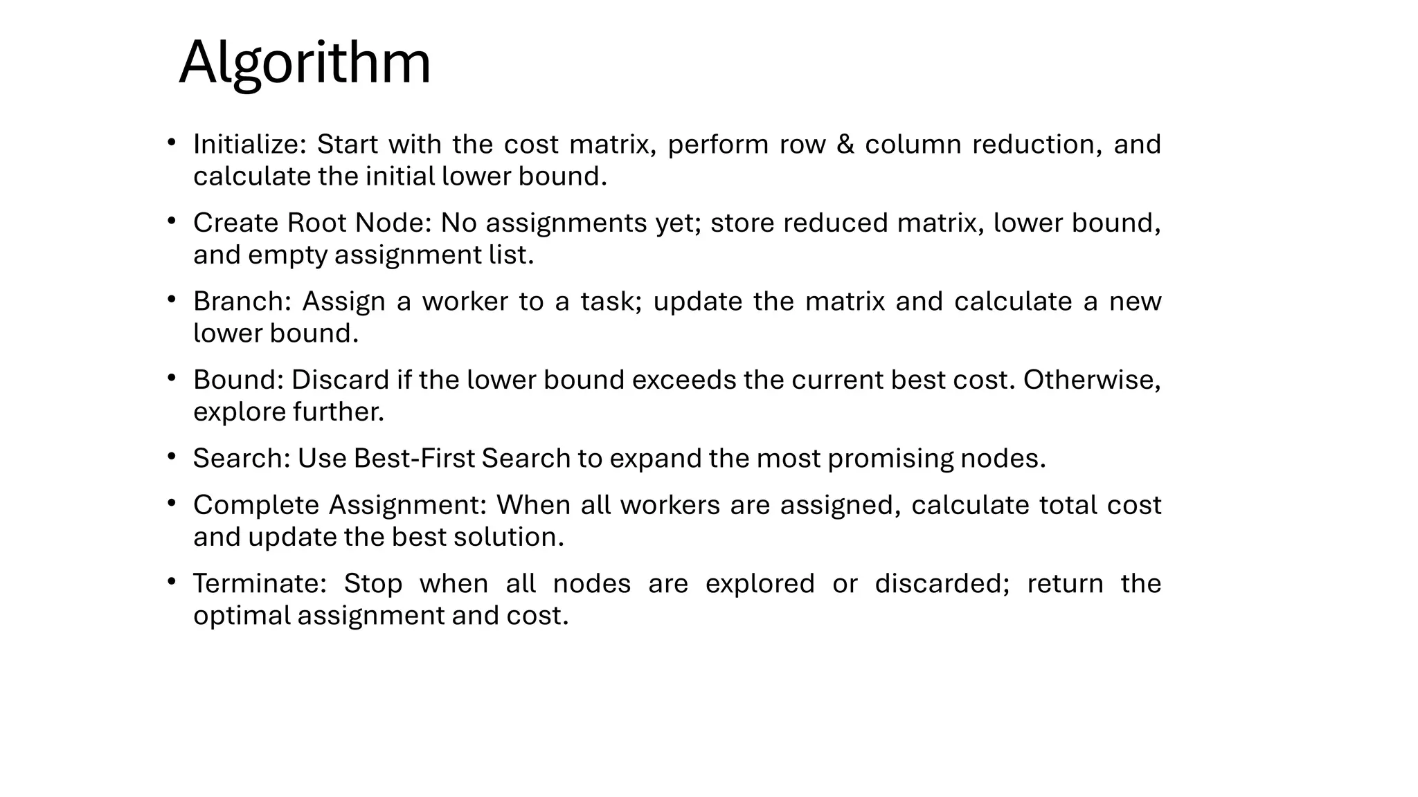
76. Algorithm
• Initialize: Start with the cost matrix, perform row & column reduction, and
calculate the initial lower bound.
• Create Root Node: No assignments yet; store reduced matrix, lower bound,
and empty assignment list.
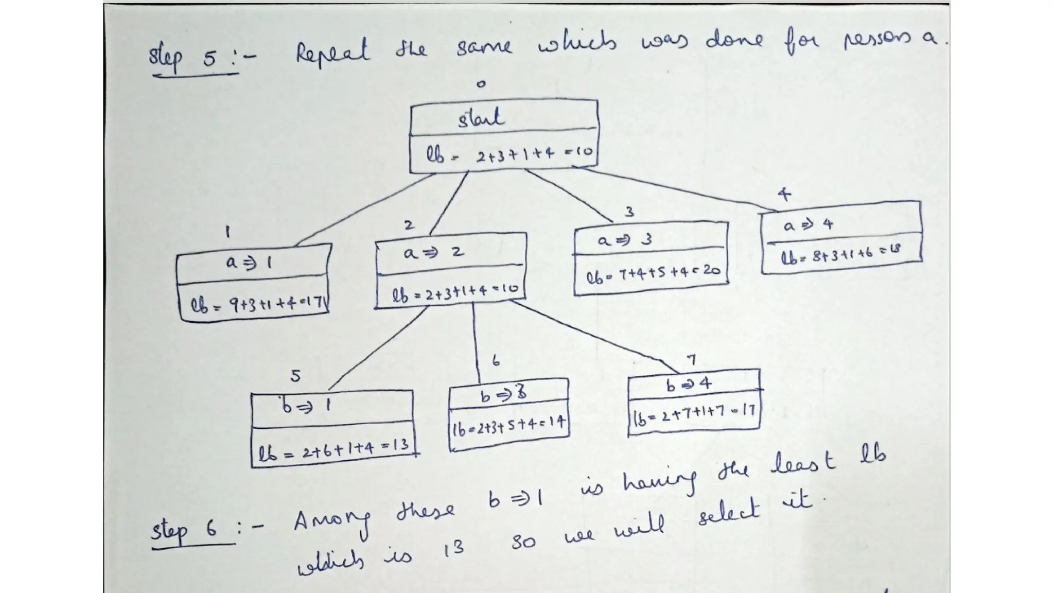
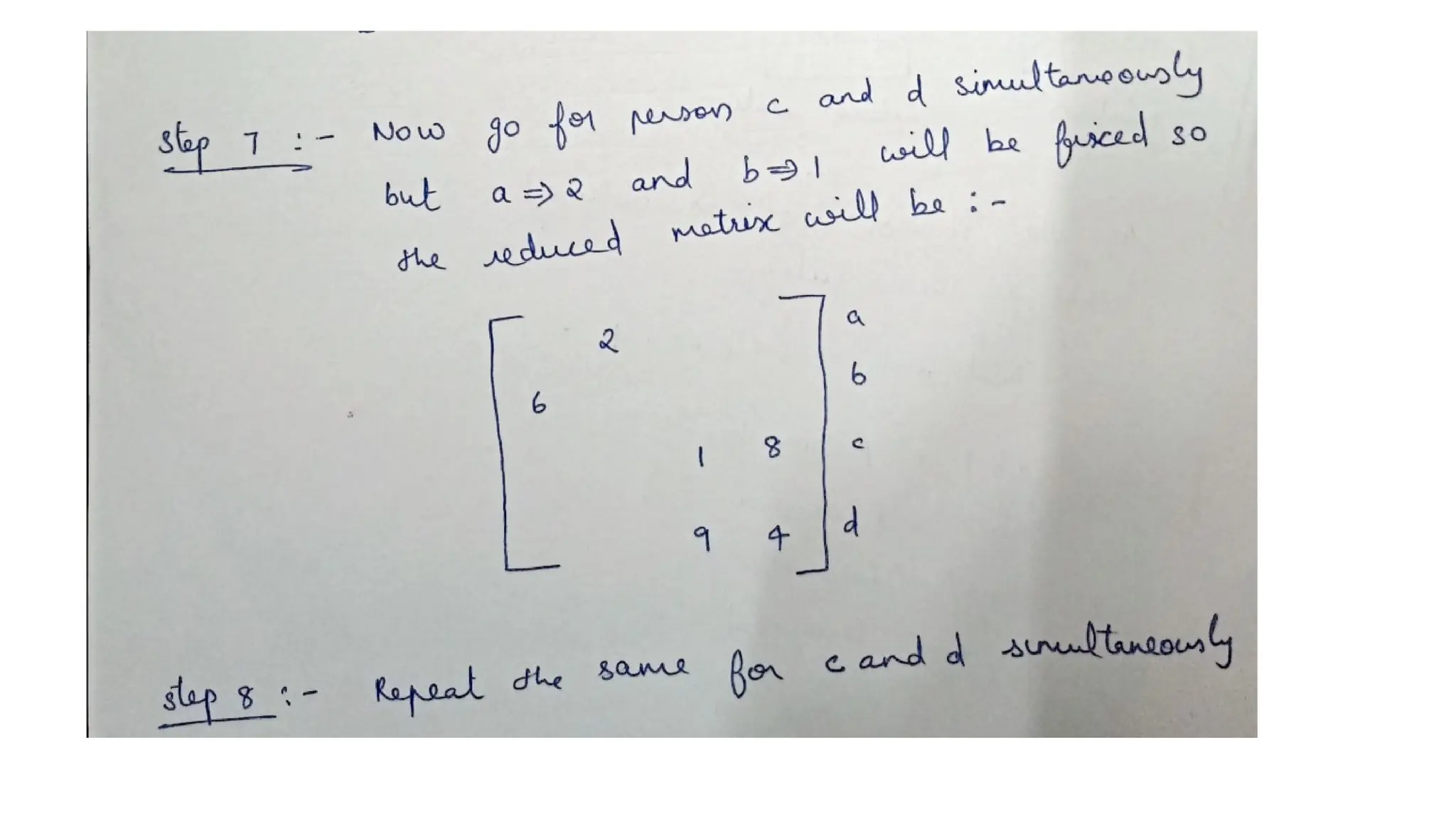
• Branch: Assign a worker to a task; update the matrix and calculate a new
lower bound.
• Bound: Discard if the lower bound exceeds the current best cost. Otherwise,
explore further.
• Search: Use Best-First Search to expand the most promising nodes.
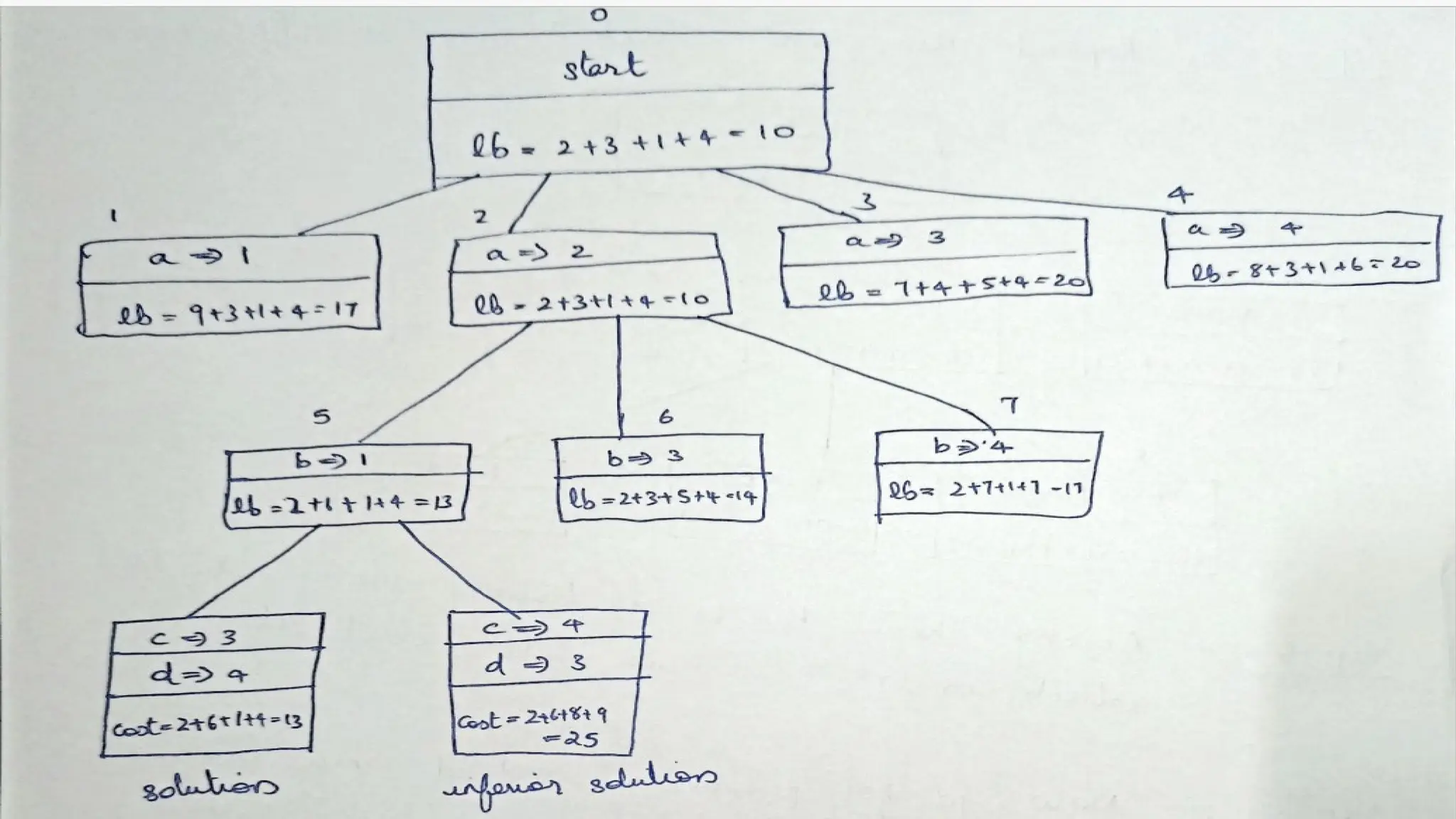
• Complete Assignment: When all workers are assigned, calculate total cost
and update the best solution.
• Terminate: Stop when all nodes are explored or discarded; return the
optimal assignment and cost.

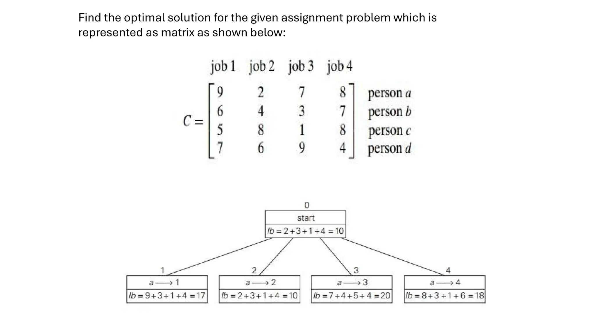
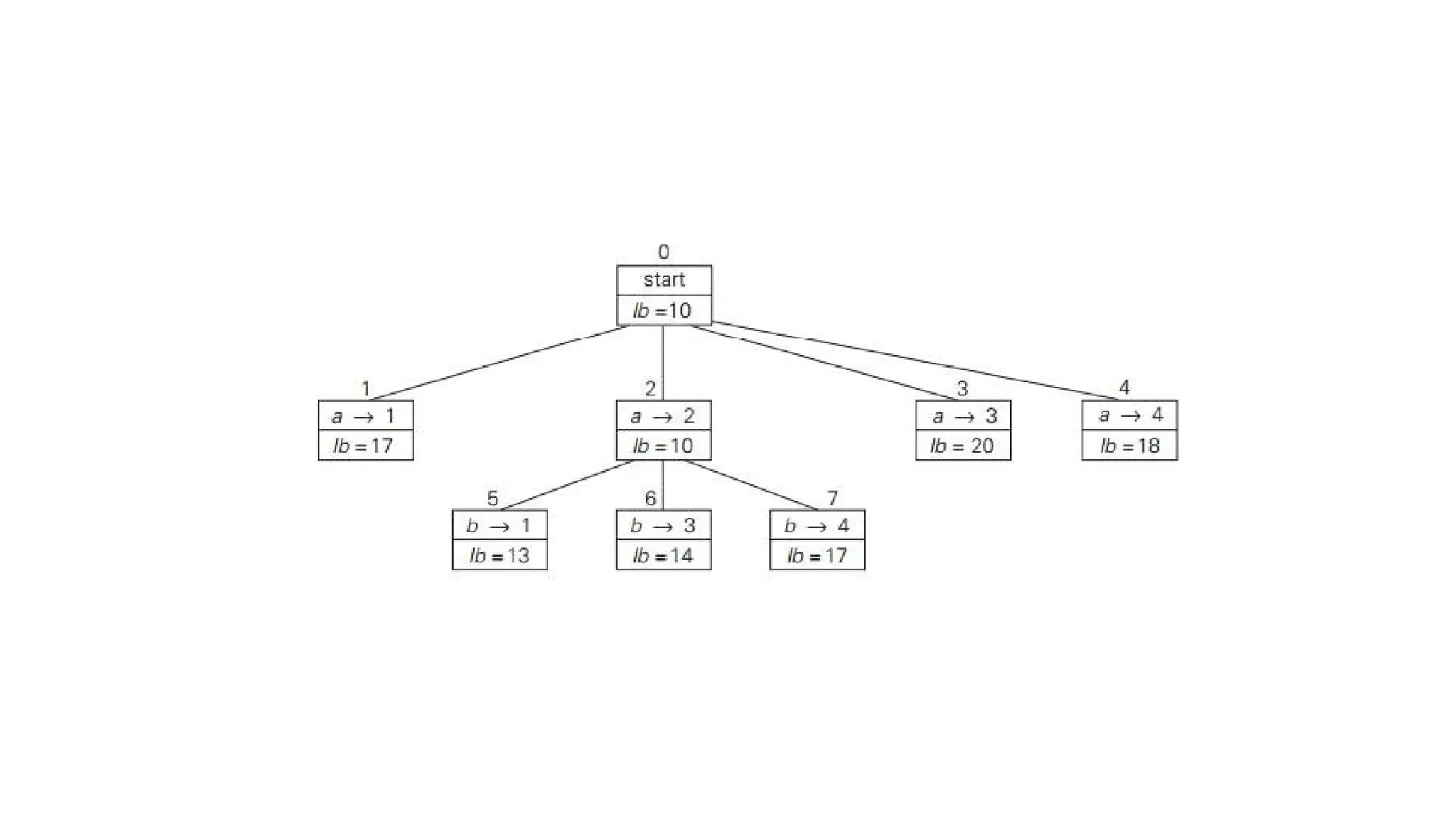
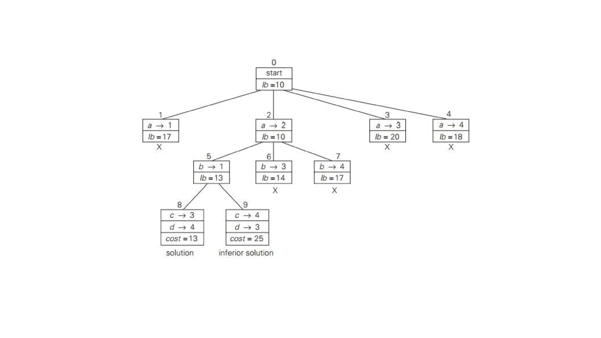
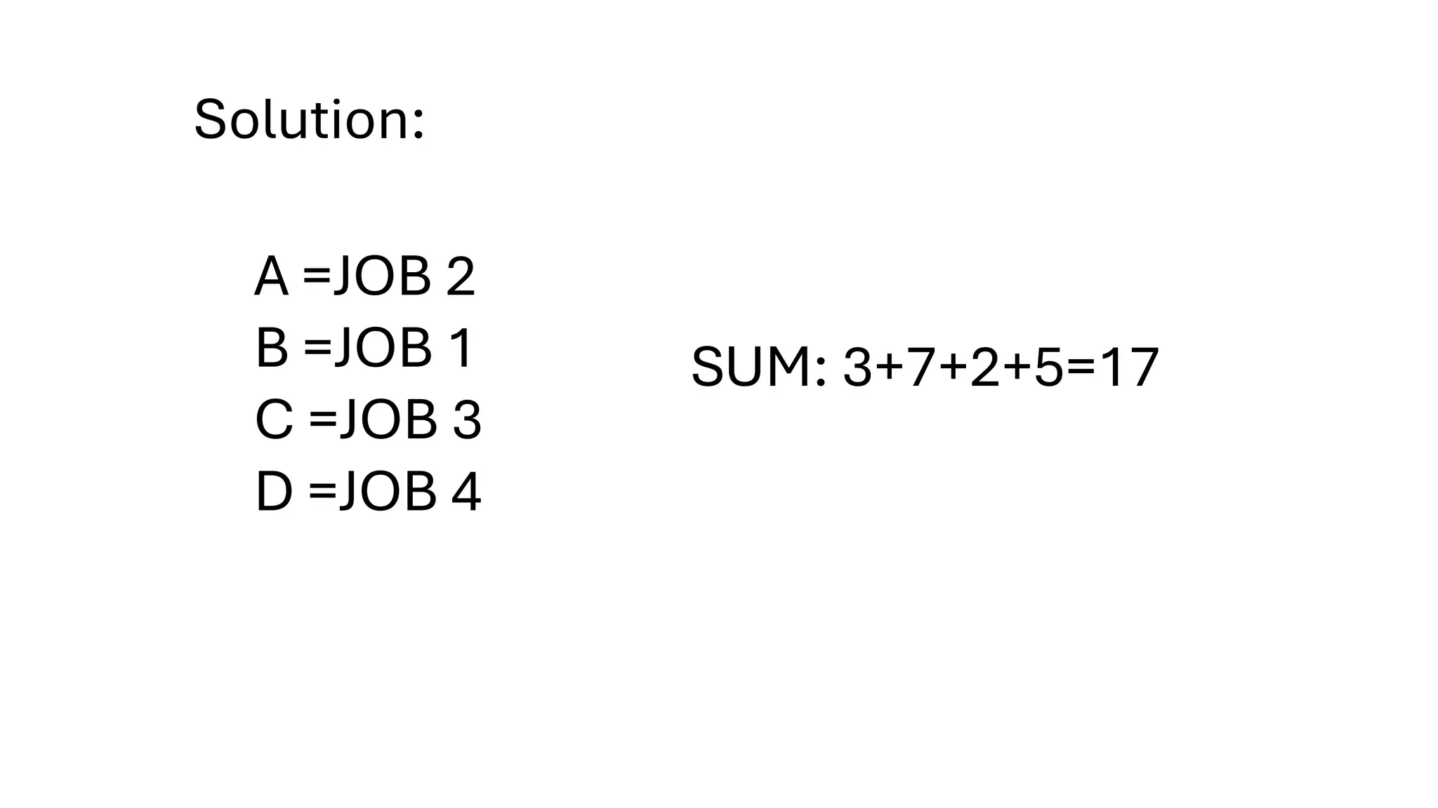
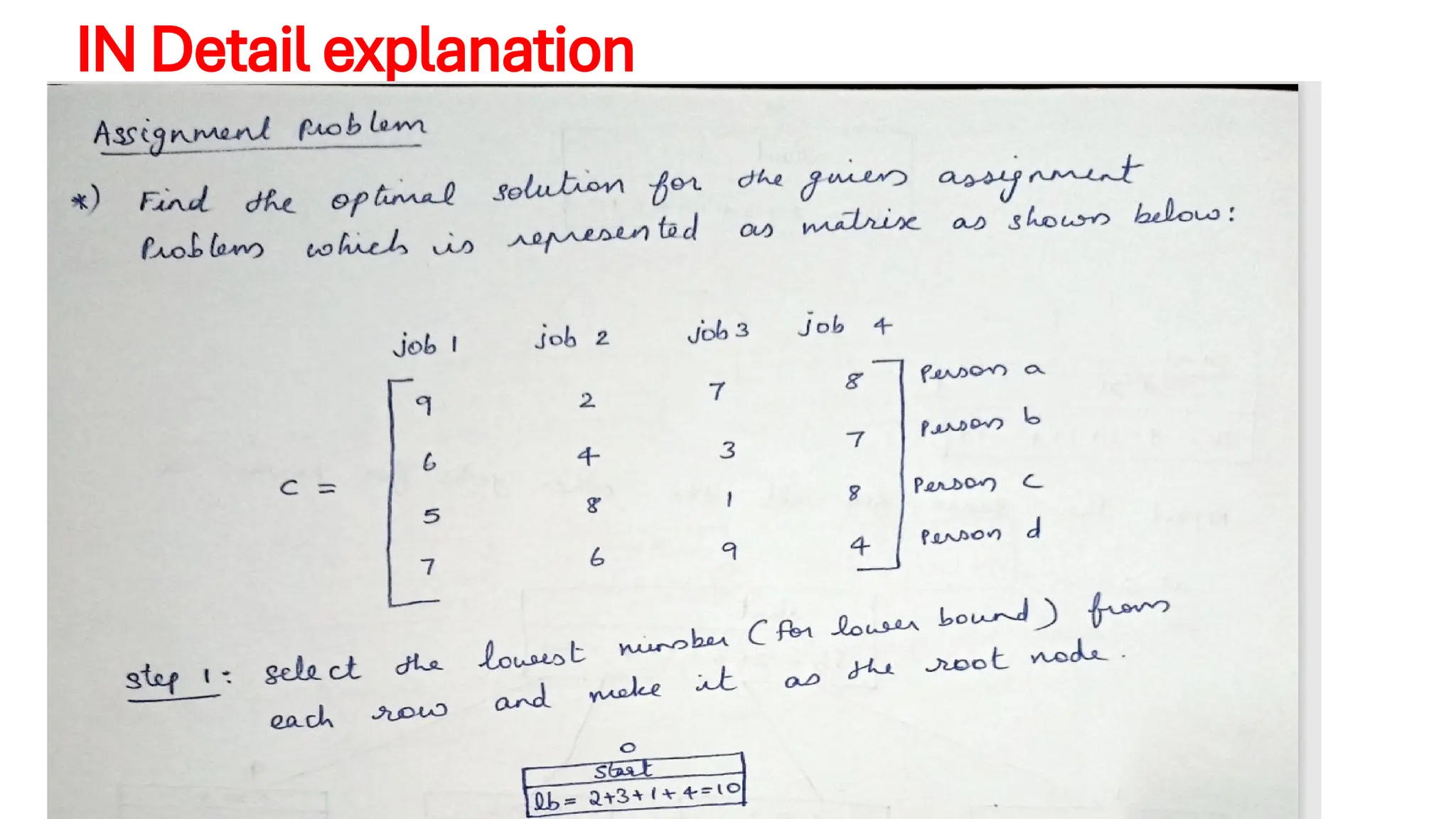
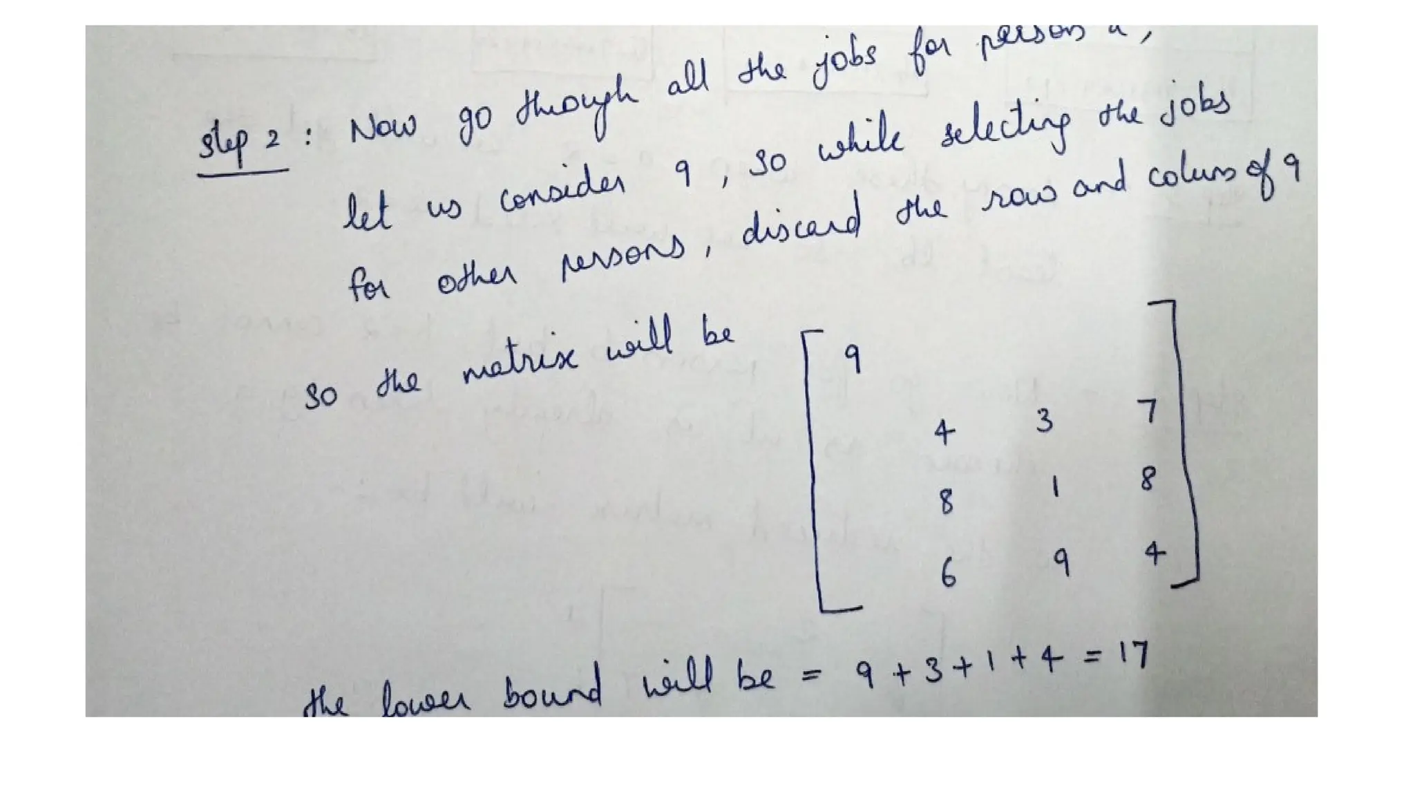
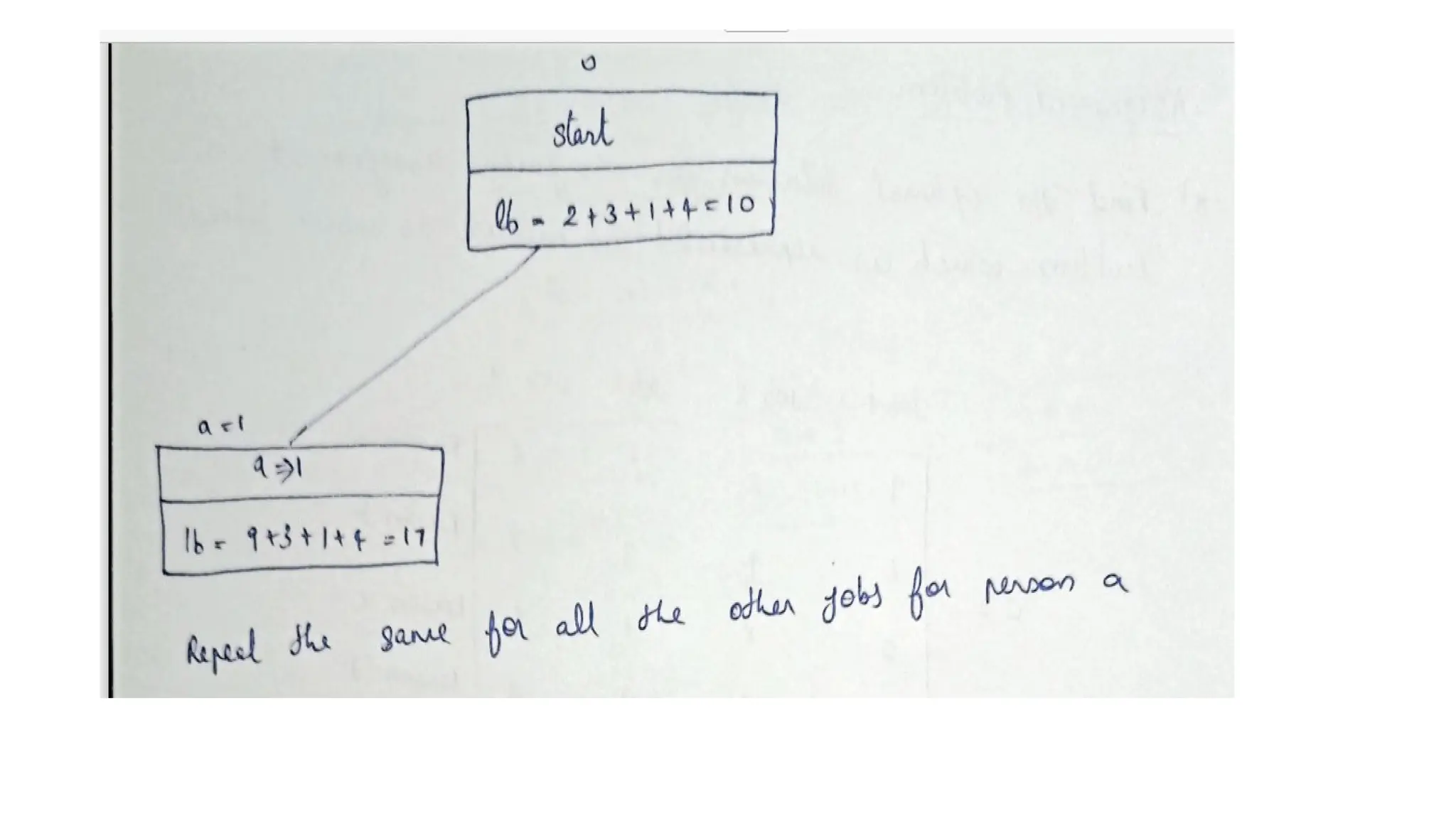
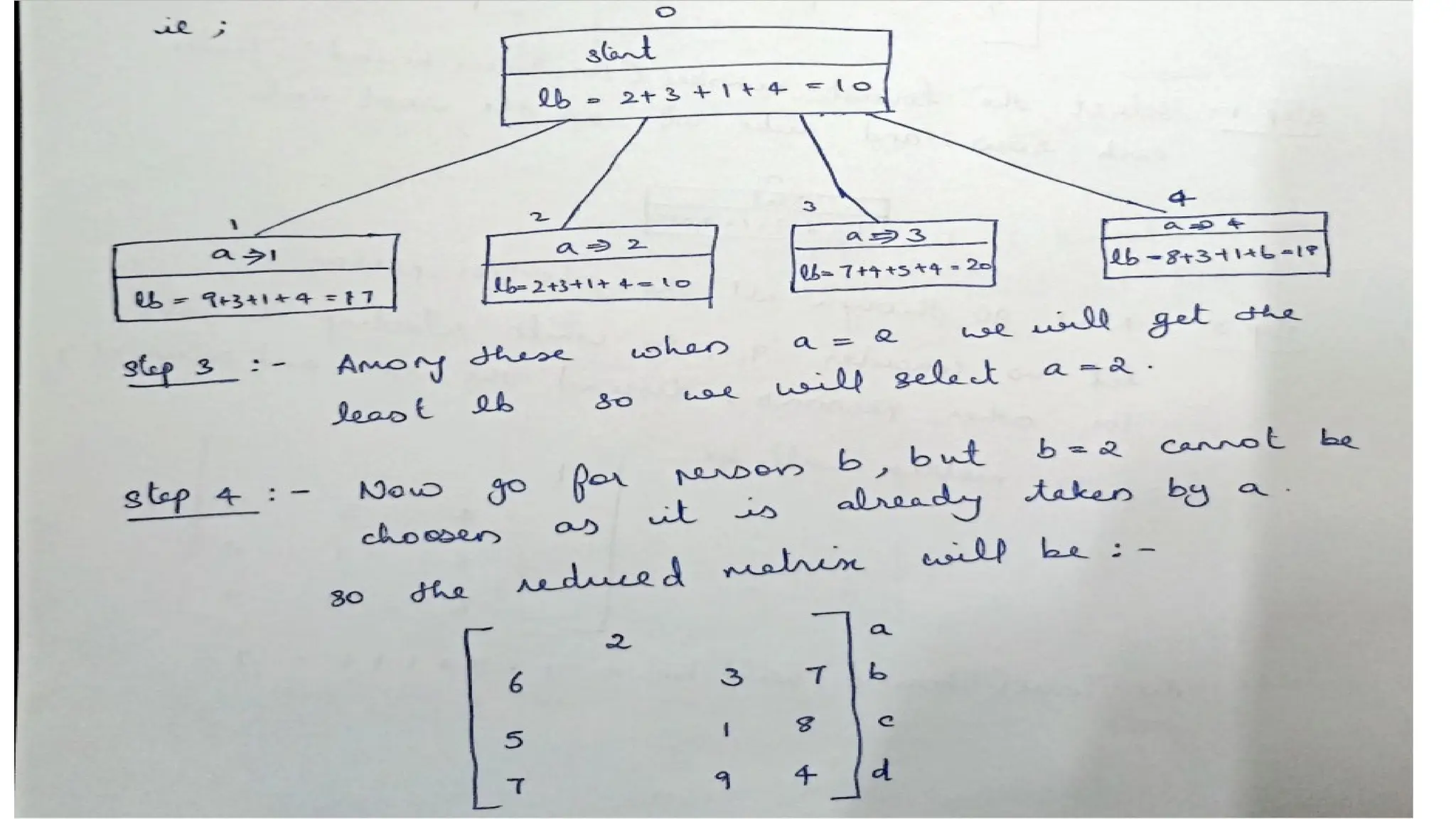
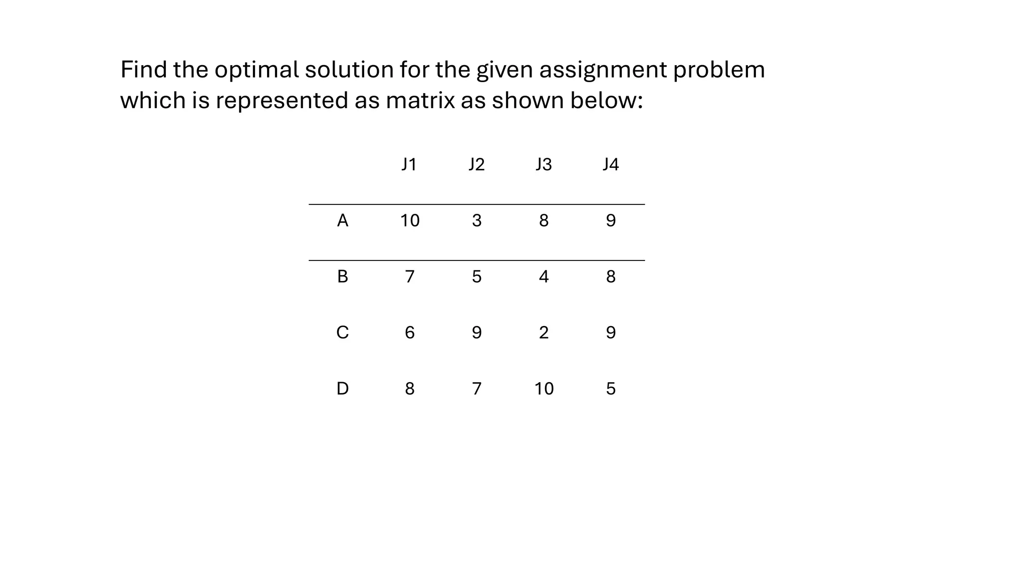
77. Find the optimal solution for the given assignment problem which is
represented as matrix as shown below:

80. IN Detail explanation

87. J1 J2 J3 J4
A 10 3 8 9
B 7 5 4 8
C 6 9 2 9
D 8 7 10 5
Find the optimal solution for the given assignment problem
which is represented as matrix as shown below:

88. Solution:
A =JOB 2
B =JOB 1
C =JOB 3
D =JOB 4
SUM: 3+7+2+5=17