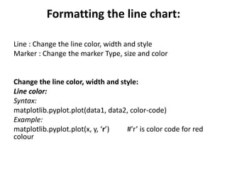
This document discusses how to create line charts, bar charts, pie charts, histograms, and scatter plots using Matplotlib in Python. It covers how to import Matplotlib, customize line styles, colors, markers, legends, titles and labels. It provides code examples for plotting single and multiple lines, formatting plots, saving figures, and using different chart types like pie charts, bar charts and histograms.

1. Plotting using Matplot Lib
Data visualization basically refers to the graphical or visual
representation of information and data using charts, graphs, maps etc.
pyplot is an interface, which exists in matplotlib library.
To draw the lines, charts etc. first of all we have to install matplotlib library in our
computer and import it in the python program.
matplotlib is a package which is used to draw 2-D graphics.
Installing the matplotlib :
Step-1: Download the wheel package of matplotlib. To download go to
the following url:
https://pypi.org/project/matplotlib/#files
Step-2: Now install it using following commands on command prompt:
python –m pip install –U pip
python –m pip install –U matplotlib

2. COMMONLY USED CHART TYPES:
• Line Chart
• Bar Chart
• Pie Chart

3. Line Chart
– A line chart displays information as a series of data points
called “markers”.
– import the matplotlib library and pyplot interface.
– pyplot interface has plot( ) function to draw a line.
– To set the lables for x-axis and y-axis, xlabel( ) and ylabel( )
functions are used.
– Use show( ) function to display the line.

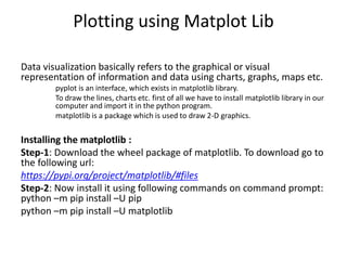
4. Line Graph
import matplotlib.pyplot as mat
x=[1,2,3]
y=[5,7,4]
mat.plot(x,y,label='First')
mat.xlabel('Cost')
mat.ylabel('Speed')
mat.title('Analysis Graph')
mat.legend()
mat.show()

6. Formatting the line chart:
Line : Change the line color, width and style
Marker : Change the marker Type, size and color
Change the line color, width and style:
Line color:
Syntax:
matplotlib.pyplot.plot(data1, data2, color-code)
Example:
matplotlib.pyplot.plot(x, y, ‘r’) #’r’ is color code for red
colour

7. color Code
Red ‘r’
Green ‘g’
Blue ‘b’
Yellow ‘y’
Magenta ‘m’
Black ‘k’
Cyan ‘c’
White ‘w’

8. Line width:
Syntax:
matplotlib.pyplot.plot(data1, data2, linewidth=value)
Example:
matplotlib.pyplot.plot(x, y, ‘c’, linewidth=6)
Line style:
Syntax:
matplotlib.pyplot.plot(data1, data2, linestyle = value)
Example:
matplotlib.pyplot.plot(x, y, ‘:’)

9. Line Style Style Name Lines
- Solid line (default) __________________
___________________
___________________
_______
-- Dashed line --------------------
: Dotted line ……………………
-. Dash-dot line -.-.-.-.-.

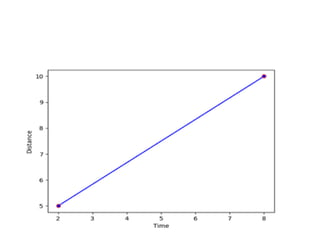
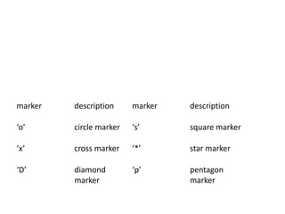
10. Change the marker type, size and
color:
To change marker type, its size and color, you can give following
additional optional arguments in plot( ) function.
marker=marker-type, markersize=value, markeredgecolor=color
Example:
import matplotlib.pyplot as pl x = [2, 8]
y = [5, 10]
pl.plot(x, y, 'b', marker='o', markersize=6, markeredgecolor='red')
pl.xlabel("Time")
pl.ylabel("Distance")
pl.show( )

12. marker description marker description
‘o’ circle marker ‘s’ square marker
‘x’ cross marker ‘*’ star marker
‘D’ diamond
marker
‘p’ pentagon
marker

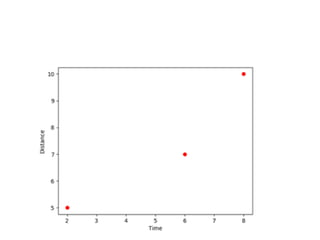
13. • Timeimport matplotlib.pyplot as pl
• x=[2,6,8]
• y=[5,7,10]
• pl.plot(x,y,'ro')
• pl.xlabel(“Time")
• pl.ylabel("Distance")
• pl.show( )

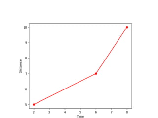
15. import matplotlib.pyplot as pl x=[2,6,8]
y=[5,7,10]
pl.plot(x,y,'ro', linestyle='-')
pl.xlabel("Time")
pl.ylabel("Distance")
pl.show( )

17. import matplotlib.pyplot as plt
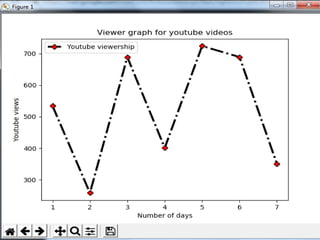
views=[534,258,689,401,724,689,350]
days=range(1,8)
plt.plot(days, views,
label='Youtube viewership', color='k', marker='D',
markerfacecolor='r',ls='-.',lw=3)
plt.xlabel ('Number of days')
plt.ylabel('Youtube views')
plt.legend()
plt.title("Viewer graph for youtube videos")
plt.show()

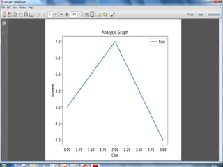
19. Save as pdf
import matplotlib.pyplot as mat
x=[1,2,3]
y=[5,7,4]
mat.plot(x,y,label='First')
mat.xlabel('Cost')
mat.ylabel('Speed')
mat.title('Analysis Graph')
mat.legend()
mat.savefig("d:/acet.pdf",format="pdf")
mat.show()

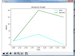
21. Plotting two lines
import matplotlib.pyplot as mat
x1=[1,2,3]
y1=[5,7,4]
x2=[1,2,3]
y2=[5,14,12]
mat.plot(x1,y1,label='First',color='cyan')
mat.plot(x2,y2,label='Second',color='g')
mat.xlabel('Cost')
mat.ylabel('Speed')
mat.title('Analysis Graph')
mat.legend()
mat.show()

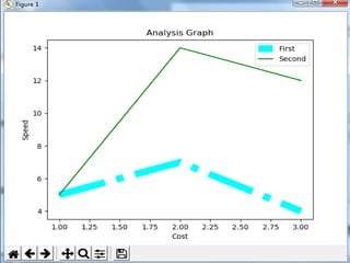
23. Line style and width
import matplotlib.pyplot as mat
x1=[1,2,3]
y1=[5,7,4]
x2=[1,2,3]
y2=[5,14,12]
mat.plot(x1,y1,label='First',color='cyan',ls='-.',linewidth=10)
mat.plot(x2,y2,label='Second',color='g')
mat.xlabel('Cost')
mat.ylabel('Speed')
mat.title('Analysis Graph')
mat.legend()
mat.show()

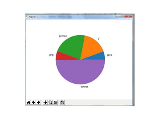
25. Pie Chart
import matplotlib.pyplot as mat
x=[11,33,44,12,99]
y=['java','c','python','php','dotnet']
mat.pie(x,labels=y)
mat.show()

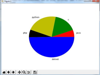
27. import matplotlib.pyplot as mat
x=[11,33,44,12,99]
y=['java','c','python','php','dotnet']
color=['red','green','y','k','b']
mat.pie(x,labels=y,colors=color)
mat.show()

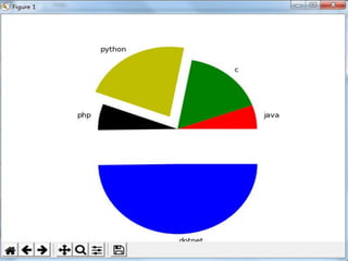
29. import matplotlib.pyplot as mat
x=[11,33,44,12,99]
y=['java','c','python','php','dotnet']
color=['red','green','y','k','b']
ex=[0,0,0.2,0,0.5]
mat.pie(x,labels=y,colors=color,explode=ex)
mat.show()

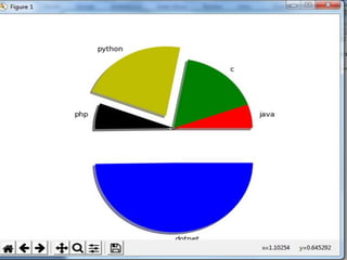
31. import matplotlib.pyplot as mat
x=[11,33,44,12,99]
y=['java','c','python','php','dotnet']
color=['red','green','y','k','b']
ex=[0,0,0.2,0,0.5]
mat.pie(x,labels=y,colors=color,explode=ex,
shadow=True)
mat.show()

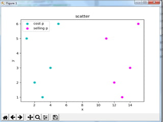
33. import matplotlib.pyplot as mat
x1=[1,2,3,4,5]
x2=[11,12,13,14,15]
y=[5,2,1,3,6]
mat.scatter(x1,y,label=“cost p",color='c')
mat.scatter(x2,y,label=“selling p",color='magenta')
mat.xlabel("x")
mat.ylabel("y")
mat.title("scatter")
mat.legend()
mat.show()

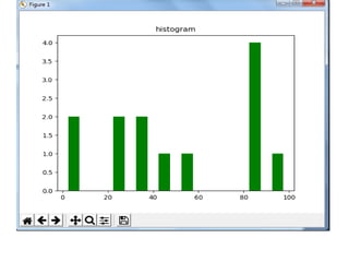
35. Histogram
import matplotlib.pyplot as mat
viewer=[24,22,33,85,41,82,55,88,1,4,99,81,38]
age=[0,10,20,30,40,50,60,70,80,90,100]
mat.hist(viewer,age,color='g',rwidth=0.5)
mat.title("histogram")
mat.show()

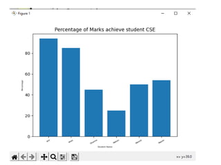
37. import matplotlib.pyplot as plt
import numpy as np
label = ['Anil', 'Vikas', 'Dharma','Mahen', 'Manish', 'Rajesh']
per = [94,85,45,25,50,54]
index = np.arange(len(label))
plt.bar(index, per)
plt.xlabel('Student Name', fontsize=5)
plt.ylabel('Percentage', fontsize=5)
plt.xticks(index, label, fontsize=5,
rotation=30)
plt.title('Percentage of Marks achieve student in ECE')
plt.show()

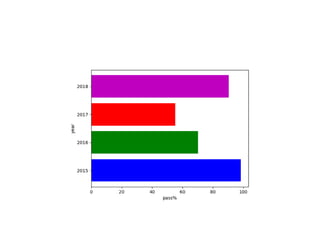
39. import matplotlib.pyplot as pl
year=['2015','2016','2017','2018']
p=[98.50,70.25,55.20,90.5]
c=['b','g','r','m']
pl.barh(year, p, color = c)
pl.xlabel("pass%")
pl.ylabel("year")
pl.show( )

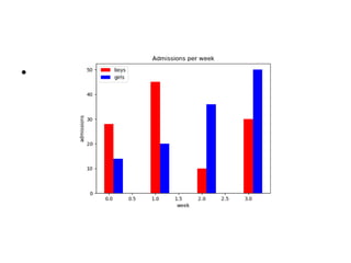
41. import matplotlib.pyplot as pl
import numpy as np
# importing numeric python for arange( )
boy=[28,45,10,30]
girl=[14,20,36,50]
X=np.arange(4) # creates a list of 4 values [0,1,2,3]
pl.bar(X, boy, width=0.2, color='r', label="boys")
pl.bar(X+0.2, girl, width=0.2,color='b',label="girls")
pl.legend(loc="upper left") # color or mark linked to
specific data range plotted at location
pl.title("Admissions per week") # title of the chart
pl.xlabel("week")
pl.ylabel("admissions")
pl.show( )

42. •

43. Location for legend
• matplotlib.pyplot.legend(loc= ‘upper left’)
• OR
• matplotlib.pyplot.legend(loc= 2)

44. location string location code
upper right 1
upper left 2
lower left 3
lower right 4
center 10

45. •Thank You