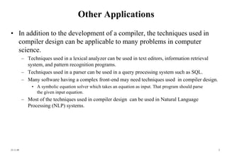
23.11.09 1
COMPILERS
• A compiler is a program takes a program written in a source language
and translates it into an equivalent program in a target language.
source program COMPILER target program
error messages
( Normally a program written in
a high-level programming language)
( Normally the equivalent program in
machine code – relocatable object file)
23.11.09 2
Other Applications
• In addition to the development of a compiler, the techniques used in
compiler design can be applicable to many problems in computer
science.
– Techniques used in a lexical analyzer can be used in text editors, information retrieval
system, and pattern recognition programs.
– Techniques used in a parser can be used in a query processing system such as SQL.
– Many software having a complex front-end may need techniques used in compiler design.
• A symbolic equation solver which takes an equation as input. That program should parse
the given input equation.
– Most of the techniques used in compiler design can be used in Natural Language
Processing (NLP) systems.
23.11.09 3
Major Parts of Compilers
• There are two major parts of a compiler: Analysis and Synthesis
• In analysis phase, an intermediate representation is created from the
given source program.
– Lexical Analyzer, Syntax Analyzer and Semantic Analyzer are the parts of this phase.
• In synthesis phase, the equivalent target program is created from this
intermediate representation.
– Intermediate Code Generator, Code Generator, and Code Optimizer are the parts of this
phase.
23.11.09 4
Phases of A Compiler
Lexical
Analyzer
Semantic
Analyzer
Syntax
Analyzer
Intermediate
Code Generator
Code
Optimizer
Code
Generator
Target
Program
Source
Program
• Each phase transforms the source program from one representation
into another representation.
• They communicate with error handlers.
• They communicate with the symbol table.
23.11.09 5
Lexical Analyzer
• Lexical Analyzer reads the source program character by character and
returns the tokens of the source program.
• A token describes a pattern of characters having same meaning in the
source program. (such as identifiers, operators, keywords, numbers,
delimeters and so on)
Ex: newval := oldval + 12 => tokens: newval identifier
:= assignment operator
oldval identifier
+ add operator
12 a number
• Puts information about identifiers into the symbol table.
• Regular expressions are used to describe tokens (lexical constructs).
• A (Deterministic) Finite State Automaton can be used in the
implementation of a lexical analyzer.
23.11.09 6
Syntax Analyzer
• A Syntax Analyzer creates the syntactic structure (generally a parse
tree) of the given program.
• A syntax analyzer is also called as a parser.
• A parse tree describes a syntactic structure.
assgstmt
identifier := expression
newval expression + expression
identifier number
oldval 12
• In a parse tree, all terminals are at leaves.
• All inner nodes are non-terminals in
a context free grammar.
23.11.09 7
Syntax Analyzer (CFG)
• The syntax of a language is specified by a context free grammar
(CFG).
• The rules in a CFG are mostly recursive.
• A syntax analyzer checks whether a given program satisfies the rules
implied by a CFG or not.
– If it satisfies, the syntax analyzer creates a parse tree for the given program.
• Ex: We use BNF (Backus Naur Form) to specify a CFG
assgstmt -> identifier := expression
expression -> identifier
expression -> number
expression -> expression + expression
23.11.09 8
Syntax Analyzer versus Lexical Analyzer
• Which constructs of a program should be recognized by the lexical
analyzer, and which ones by the syntax analyzer?
– Both of them do similar things; But the lexical analyzer deals with simple non-recursive
constructs of the language.
– The syntax analyzer deals with recursive constructs of the language.
– The lexical analyzer simplifies the job of the syntax analyzer.
– The lexical analyzer recognizes the smallest meaningful units (tokens) in a source program.
– The syntax analyzer works on the smallest meaningful units (tokens) in a source program to
recognize meaningful structures in our programming language.
23.11.09 9
Parsing Techniques
• Depending on how the parse tree is created, there are different parsing
techniques.
• These parsing techniques are categorized into two groups:
– Top-Down Parsing,
– Bottom-Up Parsing
• Top-Down Parsing:
– Construction of the parse tree starts at the root, and proceeds towards the leaves.
– Efficient top-down parsers can be easily constructed by hand.
– Recursive Predictive Parsing, Non-Recursive Predictive Parsing (LL Parsing).
• Bottom-Up Parsing:
– Construction of the parse tree starts at the leaves, and proceeds towards the root.
– Normally efficient bottom-up parsers are created with the help of some software tools.
– Bottom-up parsing is also known as shift-reduce parsing.
– Operator-Precedence Parsing – simple, restrictive, easy to implement
– LR Parsing – much general form of shift-reduce parsing, LR, SLR, LALR
23.11.09 10
Semantic Analyzer
• A semantic analyzer checks the source program for semantic errors and
collects the type information for the code generation.
• Type-checking is an important part of semantic analyzer.
• Normally semantic information cannot be represented by a context-free
language used in syntax analyzers.
• Context-free grammars used in the syntax analysis are integrated with
attributes (semantic rules)
– the result is a syntax-directed translation,
– Attribute grammars
• Ex:
newval := oldval + 12
• The type of the identifier newval must match with type of the expression (oldval+12)
23.11.09 11
Intermediate Code Generation
• A compiler may produce an explicit intermediate codes representing
the source program.
• These intermediate codes are generally machine (architecture
independent). But the level of intermediate codes is close to the level
of machine codes.
• Ex:
newval := oldval * fact + 1
id1 := id2 * id3 + 1
MULT id2,id3,temp1 Intermediates Codes (Quadraples)
ADD temp1,#1,temp2
MOV temp2,,id1
23.11.09 12
Code Optimizer (for Intermediate Code Generator)
• The code optimizer optimizes the code produced by the intermediate
code generator in the terms of time and space.
• Ex:
MULT id2,id3,temp1
ADD temp1,#1,id1
23.11.09 13
Code Generator
• Produces the target language in a specific architecture.
• The target program is normally is a relocatable object file containing
the machine codes.
• Ex:
( assume that we have an architecture with instructions whose at least one of its operands is
a machine register)
MOVE id2,R1
MULT id3,R1
ADD #1,R1
MOVE R1,id1
23.11.09 14
Lexical Analyzer
• Lexical Analyzer reads the source program character by character to
produce tokens.
• Normally a lexical analyzer doesn’t return a list of tokens at one shot,
it returns a token when the parser asks a token from it.
Lexical
Analyzer
Parser
source
program
token
get next token
23.11.09 15
Token
• Token represents a set of strings described by a pattern.
– Identifier represents a set of strings which start with a letter continues with letters and digits
– The actual string (newval) is called as lexeme.
– Tokens: identifier, number, addop, delimeter, …
• Since a token can represent more than one lexeme, additional information should be
held for that specific lexeme. This additional information is called as the attribute of
the token.
• For simplicity, a token may have a single attribute which holds the required
information for that token.
– For identifiers, this attribute a pointer to the symbol table, and the symbol table holds the actual
attributes for that token.
• Some attributes:
– <id,attr> where attr is pointer to the symbol table
– <assgop,_> no attribute is needed (if there is only one assignment operator)
– <num,val> where val is the actual value of the number.
• Token type and its attribute uniquely identifies a lexeme.
• Regular expressions are widely used to specify patterns.
23.11.09 16
Terminology of Languages
• Alphabet : a finite set of symbols (ASCII characters)
• String :
– Finite sequence of symbols on an alphabet
– Sentence and word are also used in terms of string
–  is the empty string
– |s| is the length of string s.
• Language: sets of strings over some fixed alphabet
–  the empty set is a language.
– {} the set containing empty string is a language
– The set of well-formed C programs is a language
– The set of all possible identifiers is a language.
• Operators on Strings:
– Concatenation: xy represents the concatenation of strings x and y. s  = s  s = s
– sn
= s s s .. s ( n times) s0
= 
23.11.09 17
Operations on Languages
• Concatenation:
– L1L2 = { s1s2 | s1  L1 and s2  L2 }
• Union
– L1 L2 = { s | s  L1 or s  L2 }
• Exponentiation:
– L0 = {} L1 = L L2 = LL
• Kleene Closure
– L* =
• Positive Closure
– L+ =


0
i
i
L


1
i
i
L
23.11.09 18
Example
• L1 = {a,b,c,d} L2 = {1,2}
• L1L2 = {a1,a2,b1,b2,c1,c2,d1,d2}
• L1  L2 = {a,b,c,d,1,2}
• L1
3 = all strings with length three (using a,b,c,d}
• L1
* = all strings using letters a,b,c,d and empty string
• L1
+ = doesn’t include the empty string
23.11.09 19
Regular Expressions
• We use regular expressions to describe tokens of a programming
language.
• A regular expression is built up of simpler regular expressions (using
defining rules)
• Each regular expression denotes a language.
• A language denoted by a regular expression is called as a regular set.
23.11.09 20
Regular Expressions (Rules)
Regular expressions over alphabet 
Reg. Expr Language it denotes
 {}
a  {a}
(r1) | (r2) L(r1)  L(r2)
(r1) (r2) L(r1) L(r2)
(r)* (L(r))*
(r) L(r)
• (r)+ = (r)(r)*
• (r)? = (r) | 
23.11.09 21
Regular Expressions (cont.)
• We may remove parentheses by using precedence rules.
– * highest
– concatenation next
– | lowest
• ab*|c means (a(b)*)|(c)
• Ex:
–  = {0,1}
– 0|1 => {0,1}
– (0|1)(0|1) => {00,01,10,11}
– 0* => { ,0,00,000,0000,....}
– (0|1)* => all strings with 0 and 1, including the empty string
23.11.09 22
Regular Definitions
• To write regular expression for some languages can be difficult, because
their regular expressions can be quite complex. In those cases, we may
use regular definitions.
• We can give names to regular expressions, and we can use these names
as symbols to define other regular expressions.
• A regular definition is a sequence of the definitions of the form:
d1  r1 where di is a distinct name and
d2  r2 ri is a regular expression over symbols in
. {d1,d2,...,di-1}
dn  rn
basic symbols previously defined names
23.11.09 23
Regular Definitions (cont.)
• Ex: Identifiers in Pascal
letter  A | B | ... | Z | a | b | ... | z
digit  0 | 1 | ... | 9
id  letter (letter | digit ) *
– If we try to write the regular expression representing identifiers without using regular definitions, that
regular expression will be complex.
(A|...|Z|a|...|z) ( (A|...|Z|a|...|z) | (0|...|9) ) *
• Ex: Unsigned numbers in Pascal
digit  0 | 1 | ... | 9
digits  digit +
opt-fraction  ( . digits ) ?
opt-exponent  ( E (+|-)? digits ) ?
unsigned-num  digits opt-fraction opt-exponent
23.11.09 24
Finite Automata
• A recognizer for a language is a program that takes a string x, and answers “yes” if x
is a sentence of that language, and “no” otherwise.
• We call the recognizer of the tokens as a finite automaton.
• A finite automaton can be: deterministic(DFA) or non-deterministic (NFA)
• This means that we may use a deterministic or non-deterministic automaton as a
lexical analyzer.
• Both deterministic and non-deterministic finite automaton recognize regular sets.
• Which one?
– deterministic – faster recognizer, but it may take more space
– non-deterministic – slower, but it may take less space
– Deterministic automatons are widely used lexical analyzers.
• First, we define regular expressions for tokens; Then we convert them into a DFA to
get a lexical analyzer for our tokens.
– Algorithm1: Regular Expression  NFA  DFA (two steps: first to NFA, then to DFA)
– Algorithm2: Regular Expression  DFA (directly convert a regular expression into a DFA)
23.11.09 25
Non-Deterministic Finite Automaton (NFA)
• A non-deterministic finite automaton (NFA) is a mathematical model
that consists of:
– S - a set of states
–  - a set of input symbols (alphabet)
– move – a transition function move to map state-symbol pairs to sets of states.
– s0 - a start (initial) state
– F – a set of accepting states (final states)
• - transitions are allowed in NFAs. In other words, we can move from
one state to another one without consuming any symbol.
• A NFA accepts a string x, if and only if there is a path from the starting
state to one of accepting states such that edge labels along this path spell
out x.
23.11.09 26
NFA (Example)
1
0 2
a b
start
a
b
0 is the start state s0
{2} is the set of final states F
 = {a,b}
S = {0,1,2}
Transition Function: a b
0 {0,1} {0}
1 _ {2}
2 _ _
Transition graph of the NFA
The language recognized by this NFA is (a|b)* a b
23.11.09 27
Deterministic Finite Automaton (DFA)
• A Deterministic Finite Automaton (DFA) is a special form of a NFA.
• no state has - transition
• for each symbol a and state s, there is at most one labeled edge a leaving s.
i.e. transition function is from pair of state-symbol to state (not set of states)
1
0 2
b
a
a
b
The language recognized by
this DFA is also (a|b) * a b
b a
23.11.09 28
Implementing a DFA
• Le us assume that the end of a string is marked with a special symbol
(say eos). The algorithm for recognition will be as follows: (an efficient
implementation)
s  s0 { start from the initial state }
c  nextchar { get the next character from the input string }
while (c != eos) do { do until the en dof the string }
begin
s  move(s,c) { transition function }
c  nextchar
end
if (s in F) then { if s is an accepting state }
return “yes”
else
return “no”
23.11.09 29
Implementing a NFA
S  -closure({s0}) { set all of states can be accessible from s0 by -transitions }
c  nextchar
while (c != eos) {
begin
s  -closure(move(S,c)) { set of all states can be accessible from a state in S
c  nextchar by a transition on c }
end
if (SF != ) then { if S contains an accepting state }
return “yes”
else
return “no”
• This algorithm is not efficient.
23.11.09 30
Converting A Regular Expression into A NFA
(Thomson’s Construction)
• This is one way to convert a regular expression into a NFA.
• There can be other ways (much efficient) for the conversion.
• Thomson’s Construction is simple and systematic method.
It guarantees that the resulting NFA will have exactly one final state,
and one start state.
• Construction starts from simplest parts (alphabet symbols).
To create a NFA for a complex regular expression, NFAs of its
sub-expressions are combined to create its NFA,
23.11.09 31
• To recognize an empty string 
• To recognize a symbol a in the alphabet 
• If N(r1) and N(r2) are NFAs for regular expressions r1 and r2
• For regular expression r1 | r2
a
f
i
f
i

N(r2)
N(r1)
f
i NFA for r1 | r2
Thomson’s Construction (cont.)
 


23.11.09 32
Thomson’s Construction (cont.)
• For regular expression r1 r2
i f
N(r2)
N(r1)
NFA for r1 r2
Final state of N(r2) become final state of N(r1r2)
• For regular expression r*
N(r)
i f
NFA for r*
 


23.11.09 33
Thomson’s Construction (Example - (a|b) * a )
a:
a
b
b:
(a | b)
a
b




b




a

 
(a|b) *


b




a
 

a
(a|b) * a
23.11.09 34
Converting a NFA into a DFA (subset construction)
put -closure({s0}) as an unmarked state into the set of DFA (DS)
while (there is one unmarked S1 in DS) do
begin
mark S1
for each input symbol a do
begin
S2  -closure(move(S1,a))
if (S2 is not in DS) then
add S2 into DS as an unmarked state
transfunc[S1,a]  S2
end
end
• a state S in DS is an accepting state of DFA if a state in S is an accepting state of NFA
• the start state of DFA is -closure({s0})
set of states to which there is a transition on
a from a state s in S1
-closure({s0}) is the set of all states can be accessible
from s0 by -transition.
23.11.09 35
Converting a NFA into a DFA (Example)
b




a
 

a
0 1
3
4 5
2
7 8
6
S0 = -closure({0}) = {0,1,2,4,7} S0 into DS as an unmarked state
 mark S0
-closure(move(S0,a)) = -closure({3,8}) = {1,2,3,4,6,7,8} = S1 S1 into DS
-closure(move(S0,b)) = -closure({5}) = {1,2,4,5,6,7} = S2 S2 into DS
transfunc[S0,a]  S1 transfunc[S0,b]  S2
 mark S1
-closure(move(S1,a)) = -closure({3,8}) = {1,2,3,4,6,7,8} = S1
-closure(move(S1,b)) = -closure({5}) = {1,2,4,5,6,7} = S2
transfunc[S1,a]  S1 transfunc[S1,b]  S2
 mark S2
-closure(move(S2,a)) = -closure({3,8}) = {1,2,3,4,6,7,8} = S1
-closure(move(S2,b)) = -closure({5}) = {1,2,4,5,6,7} = S2
transfunc[S2,a]  S1 transfunc[S2,b]  S2
23.11.09 36
Converting a NFA into a DFA (Example – cont.)
S0 is the start state of DFA since 0 is a member of S0={0,1,2,4,7}
S1 is an accepting state of DFA since 8 is a member of S1 = {1,2,3,4,6,7,8}
b
a
a
b
b
a
S1
S2
S0
23.11.09 37
Converting Regular Expressions Directly to DFAs
• We may convert a regular expression into a DFA (without creating a
NFA first).
• First we augment the given regular expression by concatenating it with
a special symbol #.
r  (r)# augmented regular expression
• Then, we create a syntax tree for this augmented regular expression.
• In this syntax tree, all alphabet symbols (plus # and the empty string) in
the augmented regular expression will be on the leaves, and all inner
nodes will be the operators in that augmented regular expression.
• Then each alphabet symbol (plus #) will be numbered (position
numbers).
23.11.09 38
Regular Expression  DFA (cont.)
(a|b) * a  (a|b) * a # augmented regular expression

*

|
b
a
#
a
1
4
3
2
Syntax tree of (a|b) * a #
• each symbol is numbered (positions)
• each symbol is at a leave
• inner nodes are operators
23.11.09 39
followpos
Then we define the function followpos for the positions (positions
assigned to leaves).
followpos(i) -- is the set of positions which can follow
the position i in the strings generated by
the augmented regular expression.
For example, ( a | b) * a #
1 2 3 4
followpos(1) = {1,2,3}
followpos(2) = {1,2,3}
followpos(3) = {4}
followpos(4) = {}
followpos is just defined for leaves,
it is not defined for inner nodes.
23.11.09 40
firstpos, lastpos, nullable
• To evaluate followpos, we need three more functions to be defined for
the nodes (not just for leaves) of the syntax tree.
• firstpos(n) -- the set of the positions of the first symbols of strings
generated by the sub-expression rooted by n.
• lastpos(n) -- the set of the positions of the last symbols of strings
generated by the sub-expression rooted by n.
• nullable(n) -- true if the empty string is a member of strings
generated by the sub-expression rooted by n
false otherwise
23.11.09 41
How to evaluate firstpos, lastpos, nullable
n nullable(n) firstpos(n) lastpos(n)
leaf labeled  true  
leaf labeled
with position i
false {i} {i}
|
c1 c2
nullable(c1) or
nullable(c2)
firstpos(c1)  firstpos(c2) lastpos(c1)  lastpos(c2)

c1 c2
nullable(c1) and
nullable(c2)
if (nullable(c1))
firstpos(c1)  firstpos(c2)
else firstpos(c1)
if (nullable(c2))
lastpos(c1)  lastpos(c2)
else lastpos(c2)
*
c1
true firstpos(c1) lastpos(c1)
23.11.09 42
How to evaluate followpos
• Two-rules define the function followpos:
1. If n is concatenation-node with left child c1 and right child c2,
and i is a position in lastpos(c1), then all positions in firstpos(c2) are in
followpos(i).
2. If n is a star-node, and i is a position in lastpos(n), then all positions in
firstpos(n) are in followpos(i).
• If firstpos and lastpos have been computed for each node, followpos
of each position can be computed by making one depth-first traversal
of the syntax tree.
23.11.09 43
Example -- ( a | b) * a #

*

|
b
a
#
a
1
4
3
2
{1}
{1}
{1,2,3}
{3}
{1,2,3}
{1,2}
{1,2}
{2}
{4}
{4}
{4}
{3}
{3}
{1,2}
{1,2}
{2}
green – firstpos
blue – lastpos
Then we can calculate followpos
followpos(1) = {1,2,3}
followpos(2) = {1,2,3}
followpos(3) = {4}
followpos(4) = {}
• After we calculate follow positions, we are ready to create DFA
for the regular expression.
23.11.09 44
Algorithm (RE  DFA)
• Create the syntax tree of (r) #
• Calculate the functions: followpos, firstpos, lastpos, nullable
• Put firstpos(root) into the states of DFA as an unmarked state.
• while (there is an unmarked state S in the states of DFA) do
– mark S
– for each input symbol a do
• let s1,...,sn are positions in S and symbols in those positions are a
• S’  followpos(s1)  ...  followpos(sn)
• move(S,a)  S’
• if (S’ is not empty and not in the states of DFA)
– put S’ into the states of DFA as an unmarked state.
• the start state of DFA is firstpos(root)
• the accepting states of DFA are all states containing the position of #
23.11.09 45
Example -- ( a | b) * a #
followpos(1)={1,2,3} followpos(2)={1,2,3} followpos(3)={4} followpos(4)={}
S1=firstpos(root)={1,2,3}
 mark S1
a: followpos(1)  followpos(3)={1,2,3,4}=S2 move(S1,a)=S2
b: followpos(2)={1,2,3}=S1 move(S1,b)=S1
 mark S2
a: followpos(1)  followpos(3)={1,2,3,4}=S2 move(S2,a)=S2
b: followpos(2)={1,2,3}=S1 move(S2,b)=S1
start state: S1
accepting states: {S2}
1 2 3 4
S1 S2
a
b
b
a
23.11.09 46
Example -- ( a | ) b c* #
1 2 3 4
followpos(1)={2} followpos(2)={3,4} followpos(3)={3,4} followpos(4)={}
S1=firstpos(root)={1,2}
 mark S1
a: followpos(1)={2}=S2 move(S1,a)=S2
b: followpos(2)={3,4}=S3 move(S1,b)=S3
 mark S2
b: followpos(2)={3,4}=S3 move(S2,b)=S3
 mark S3
c: followpos(3)={3,4}=S3 move(S3,c)=S3
start state: S1
accepting states: {S3}
S3
S2
S1
c
a
b
b
23.11.09 47
Minimizing Number of States of a DFA
• partition the set of states into two groups:
– G1 : set of accepting states
– G2 : set of non-accepting states
• For each new group G
– partition G into subgroups such that states s1 and s2 are in the same group iff
for all input symbols a, states s1 and s2 have transitions to states in the same group.
• Start state of the minimized DFA is the group containing
the start state of the original DFA.
• Accepting states of the minimized DFA are the groups containing
the accepting states of the original DFA.
23.11.09 48
Minimizing DFA - Example
b a
a
a
b
b
3
2
1
G1 = {2}
G2 = {1,3}
G2 cannot be partitioned because
move(1,a)=2 move(1,b)=3
move(3,a)=2 move(2,b)=3
So, the minimized DFA (with minimum states)
{1,3}
a
a
b
b
{2}
23.11.09 49
Minimizing DFA – Another Example
b
b
b
a
a
a
a
b 4
3
2
1
Groups: {1,2,3} {4}
a b
1->2 1->3
2->2 2->3
3->4 3->3
{1,2} {3}
no more partitioning
So, the minimized DFA
{1,2}
{4}
{3}
b
a
a
a
b
b
23.11.09 50
Some Other Issues in Lexical Analyzer
• The lexical analyzer has to recognize the longest possible string.
– Ex: identifier newval -- n ne new newv newva newval
• What is the end of a token? Is there any character which marks the end
of a token?
– It is normally not defined.
– If the number of characters in a token is fixed, in that case no problem: + -
– But <  < or <> (in Pascal)
– The end of an identifier : the characters cannot be in an identifier can mark the end of token.
– We may need a lookhead
• In Prolog: p :- X is 1. p :- X is 1.5.
The dot followed by a white space character can mark the end of a number.
But if that is not the case, the dot must be treated as a part of the number.
23.11.09 51
Some Other Issues in Lexical Analyzer (cont.)
• Skipping comments
– Normally we don’t return a comment as a token.
– We skip a comment, and return the next token (which is not a comment) to the parser.
– So, the comments are only processed by the lexical analyzer, and the don’t complicate
the syntax of the language.
• Symbol table interface
– symbol table holds information about tokens (at least lexeme of identifiers)
– how to implement the symbol table, and what kind of operations.
• hash table – open addressing, chaining
• putting into the hash table, finding the position of a token from its lexeme.
• Positions of the tokens in the file (for the error handling).
23.11.09 52
Syntax Analysis
Context Free Grammars
Top-Down Parsing, LL Parsing
Bottom-Up Parsing, LR Parsing
Syntax-Directed Translation
Attribute Definitions
Evaluation of Attribute Definitions
Semantic Analysis, Type Checking
Run-Time Organization
Intermediate Code Generation

Unit1.ppt

  • 1.
    23.11.09 1 COMPILERS • Acompiler is a program takes a program written in a source language and translates it into an equivalent program in a target language. source program COMPILER target program error messages ( Normally a program written in a high-level programming language) ( Normally the equivalent program in machine code – relocatable object file)
  • 2.
    23.11.09 2 Other Applications •In addition to the development of a compiler, the techniques used in compiler design can be applicable to many problems in computer science. – Techniques used in a lexical analyzer can be used in text editors, information retrieval system, and pattern recognition programs. – Techniques used in a parser can be used in a query processing system such as SQL. – Many software having a complex front-end may need techniques used in compiler design. • A symbolic equation solver which takes an equation as input. That program should parse the given input equation. – Most of the techniques used in compiler design can be used in Natural Language Processing (NLP) systems.
  • 3.
    23.11.09 3 Major Partsof Compilers • There are two major parts of a compiler: Analysis and Synthesis • In analysis phase, an intermediate representation is created from the given source program. – Lexical Analyzer, Syntax Analyzer and Semantic Analyzer are the parts of this phase. • In synthesis phase, the equivalent target program is created from this intermediate representation. – Intermediate Code Generator, Code Generator, and Code Optimizer are the parts of this phase.
  • 4.
    23.11.09 4 Phases ofA Compiler Lexical Analyzer Semantic Analyzer Syntax Analyzer Intermediate Code Generator Code Optimizer Code Generator Target Program Source Program • Each phase transforms the source program from one representation into another representation. • They communicate with error handlers. • They communicate with the symbol table.
  • 5.
    23.11.09 5 Lexical Analyzer •Lexical Analyzer reads the source program character by character and returns the tokens of the source program. • A token describes a pattern of characters having same meaning in the source program. (such as identifiers, operators, keywords, numbers, delimeters and so on) Ex: newval := oldval + 12 => tokens: newval identifier := assignment operator oldval identifier + add operator 12 a number • Puts information about identifiers into the symbol table. • Regular expressions are used to describe tokens (lexical constructs). • A (Deterministic) Finite State Automaton can be used in the implementation of a lexical analyzer.
  • 6.
    23.11.09 6 Syntax Analyzer •A Syntax Analyzer creates the syntactic structure (generally a parse tree) of the given program. • A syntax analyzer is also called as a parser. • A parse tree describes a syntactic structure. assgstmt identifier := expression newval expression + expression identifier number oldval 12 • In a parse tree, all terminals are at leaves. • All inner nodes are non-terminals in a context free grammar.
  • 7.
    23.11.09 7 Syntax Analyzer(CFG) • The syntax of a language is specified by a context free grammar (CFG). • The rules in a CFG are mostly recursive. • A syntax analyzer checks whether a given program satisfies the rules implied by a CFG or not. – If it satisfies, the syntax analyzer creates a parse tree for the given program. • Ex: We use BNF (Backus Naur Form) to specify a CFG assgstmt -> identifier := expression expression -> identifier expression -> number expression -> expression + expression
  • 8.
    23.11.09 8 Syntax Analyzerversus Lexical Analyzer • Which constructs of a program should be recognized by the lexical analyzer, and which ones by the syntax analyzer? – Both of them do similar things; But the lexical analyzer deals with simple non-recursive constructs of the language. – The syntax analyzer deals with recursive constructs of the language. – The lexical analyzer simplifies the job of the syntax analyzer. – The lexical analyzer recognizes the smallest meaningful units (tokens) in a source program. – The syntax analyzer works on the smallest meaningful units (tokens) in a source program to recognize meaningful structures in our programming language.
  • 9.
    23.11.09 9 Parsing Techniques •Depending on how the parse tree is created, there are different parsing techniques. • These parsing techniques are categorized into two groups: – Top-Down Parsing, – Bottom-Up Parsing • Top-Down Parsing: – Construction of the parse tree starts at the root, and proceeds towards the leaves. – Efficient top-down parsers can be easily constructed by hand. – Recursive Predictive Parsing, Non-Recursive Predictive Parsing (LL Parsing). • Bottom-Up Parsing: – Construction of the parse tree starts at the leaves, and proceeds towards the root. – Normally efficient bottom-up parsers are created with the help of some software tools. – Bottom-up parsing is also known as shift-reduce parsing. – Operator-Precedence Parsing – simple, restrictive, easy to implement – LR Parsing – much general form of shift-reduce parsing, LR, SLR, LALR
  • 10.
    23.11.09 10 Semantic Analyzer •A semantic analyzer checks the source program for semantic errors and collects the type information for the code generation. • Type-checking is an important part of semantic analyzer. • Normally semantic information cannot be represented by a context-free language used in syntax analyzers. • Context-free grammars used in the syntax analysis are integrated with attributes (semantic rules) – the result is a syntax-directed translation, – Attribute grammars • Ex: newval := oldval + 12 • The type of the identifier newval must match with type of the expression (oldval+12)
  • 11.
    23.11.09 11 Intermediate CodeGeneration • A compiler may produce an explicit intermediate codes representing the source program. • These intermediate codes are generally machine (architecture independent). But the level of intermediate codes is close to the level of machine codes. • Ex: newval := oldval * fact + 1 id1 := id2 * id3 + 1 MULT id2,id3,temp1 Intermediates Codes (Quadraples) ADD temp1,#1,temp2 MOV temp2,,id1
  • 12.
    23.11.09 12 Code Optimizer(for Intermediate Code Generator) • The code optimizer optimizes the code produced by the intermediate code generator in the terms of time and space. • Ex: MULT id2,id3,temp1 ADD temp1,#1,id1
  • 13.
    23.11.09 13 Code Generator •Produces the target language in a specific architecture. • The target program is normally is a relocatable object file containing the machine codes. • Ex: ( assume that we have an architecture with instructions whose at least one of its operands is a machine register) MOVE id2,R1 MULT id3,R1 ADD #1,R1 MOVE R1,id1
  • 14.
    23.11.09 14 Lexical Analyzer •Lexical Analyzer reads the source program character by character to produce tokens. • Normally a lexical analyzer doesn’t return a list of tokens at one shot, it returns a token when the parser asks a token from it. Lexical Analyzer Parser source program token get next token
  • 15.
    23.11.09 15 Token • Tokenrepresents a set of strings described by a pattern. – Identifier represents a set of strings which start with a letter continues with letters and digits – The actual string (newval) is called as lexeme. – Tokens: identifier, number, addop, delimeter, … • Since a token can represent more than one lexeme, additional information should be held for that specific lexeme. This additional information is called as the attribute of the token. • For simplicity, a token may have a single attribute which holds the required information for that token. – For identifiers, this attribute a pointer to the symbol table, and the symbol table holds the actual attributes for that token. • Some attributes: – <id,attr> where attr is pointer to the symbol table – <assgop,_> no attribute is needed (if there is only one assignment operator) – <num,val> where val is the actual value of the number. • Token type and its attribute uniquely identifies a lexeme. • Regular expressions are widely used to specify patterns.
  • 16.
    23.11.09 16 Terminology ofLanguages • Alphabet : a finite set of symbols (ASCII characters) • String : – Finite sequence of symbols on an alphabet – Sentence and word are also used in terms of string –  is the empty string – |s| is the length of string s. • Language: sets of strings over some fixed alphabet –  the empty set is a language. – {} the set containing empty string is a language – The set of well-formed C programs is a language – The set of all possible identifiers is a language. • Operators on Strings: – Concatenation: xy represents the concatenation of strings x and y. s  = s  s = s – sn = s s s .. s ( n times) s0 = 
  • 17.
    23.11.09 17 Operations onLanguages • Concatenation: – L1L2 = { s1s2 | s1  L1 and s2  L2 } • Union – L1 L2 = { s | s  L1 or s  L2 } • Exponentiation: – L0 = {} L1 = L L2 = LL • Kleene Closure – L* = • Positive Closure – L+ =   0 i i L   1 i i L
  • 18.
    23.11.09 18 Example • L1= {a,b,c,d} L2 = {1,2} • L1L2 = {a1,a2,b1,b2,c1,c2,d1,d2} • L1  L2 = {a,b,c,d,1,2} • L1 3 = all strings with length three (using a,b,c,d} • L1 * = all strings using letters a,b,c,d and empty string • L1 + = doesn’t include the empty string
  • 19.
    23.11.09 19 Regular Expressions •We use regular expressions to describe tokens of a programming language. • A regular expression is built up of simpler regular expressions (using defining rules) • Each regular expression denotes a language. • A language denoted by a regular expression is called as a regular set.
  • 20.
    23.11.09 20 Regular Expressions(Rules) Regular expressions over alphabet  Reg. Expr Language it denotes  {} a  {a} (r1) | (r2) L(r1)  L(r2) (r1) (r2) L(r1) L(r2) (r)* (L(r))* (r) L(r) • (r)+ = (r)(r)* • (r)? = (r) | 
  • 21.
    23.11.09 21 Regular Expressions(cont.) • We may remove parentheses by using precedence rules. – * highest – concatenation next – | lowest • ab*|c means (a(b)*)|(c) • Ex: –  = {0,1} – 0|1 => {0,1} – (0|1)(0|1) => {00,01,10,11} – 0* => { ,0,00,000,0000,....} – (0|1)* => all strings with 0 and 1, including the empty string
  • 22.
    23.11.09 22 Regular Definitions •To write regular expression for some languages can be difficult, because their regular expressions can be quite complex. In those cases, we may use regular definitions. • We can give names to regular expressions, and we can use these names as symbols to define other regular expressions. • A regular definition is a sequence of the definitions of the form: d1  r1 where di is a distinct name and d2  r2 ri is a regular expression over symbols in . {d1,d2,...,di-1} dn  rn basic symbols previously defined names
  • 23.
    23.11.09 23 Regular Definitions(cont.) • Ex: Identifiers in Pascal letter  A | B | ... | Z | a | b | ... | z digit  0 | 1 | ... | 9 id  letter (letter | digit ) * – If we try to write the regular expression representing identifiers without using regular definitions, that regular expression will be complex. (A|...|Z|a|...|z) ( (A|...|Z|a|...|z) | (0|...|9) ) * • Ex: Unsigned numbers in Pascal digit  0 | 1 | ... | 9 digits  digit + opt-fraction  ( . digits ) ? opt-exponent  ( E (+|-)? digits ) ? unsigned-num  digits opt-fraction opt-exponent
  • 24.
    23.11.09 24 Finite Automata •A recognizer for a language is a program that takes a string x, and answers “yes” if x is a sentence of that language, and “no” otherwise. • We call the recognizer of the tokens as a finite automaton. • A finite automaton can be: deterministic(DFA) or non-deterministic (NFA) • This means that we may use a deterministic or non-deterministic automaton as a lexical analyzer. • Both deterministic and non-deterministic finite automaton recognize regular sets. • Which one? – deterministic – faster recognizer, but it may take more space – non-deterministic – slower, but it may take less space – Deterministic automatons are widely used lexical analyzers. • First, we define regular expressions for tokens; Then we convert them into a DFA to get a lexical analyzer for our tokens. – Algorithm1: Regular Expression  NFA  DFA (two steps: first to NFA, then to DFA) – Algorithm2: Regular Expression  DFA (directly convert a regular expression into a DFA)
  • 25.
    23.11.09 25 Non-Deterministic FiniteAutomaton (NFA) • A non-deterministic finite automaton (NFA) is a mathematical model that consists of: – S - a set of states –  - a set of input symbols (alphabet) – move – a transition function move to map state-symbol pairs to sets of states. – s0 - a start (initial) state – F – a set of accepting states (final states) • - transitions are allowed in NFAs. In other words, we can move from one state to another one without consuming any symbol. • A NFA accepts a string x, if and only if there is a path from the starting state to one of accepting states such that edge labels along this path spell out x.
  • 26.
    23.11.09 26 NFA (Example) 1 02 a b start a b 0 is the start state s0 {2} is the set of final states F  = {a,b} S = {0,1,2} Transition Function: a b 0 {0,1} {0} 1 _ {2} 2 _ _ Transition graph of the NFA The language recognized by this NFA is (a|b)* a b
  • 27.
    23.11.09 27 Deterministic FiniteAutomaton (DFA) • A Deterministic Finite Automaton (DFA) is a special form of a NFA. • no state has - transition • for each symbol a and state s, there is at most one labeled edge a leaving s. i.e. transition function is from pair of state-symbol to state (not set of states) 1 0 2 b a a b The language recognized by this DFA is also (a|b) * a b b a
  • 28.
    23.11.09 28 Implementing aDFA • Le us assume that the end of a string is marked with a special symbol (say eos). The algorithm for recognition will be as follows: (an efficient implementation) s  s0 { start from the initial state } c  nextchar { get the next character from the input string } while (c != eos) do { do until the en dof the string } begin s  move(s,c) { transition function } c  nextchar end if (s in F) then { if s is an accepting state } return “yes” else return “no”
  • 29.
    23.11.09 29 Implementing aNFA S  -closure({s0}) { set all of states can be accessible from s0 by -transitions } c  nextchar while (c != eos) { begin s  -closure(move(S,c)) { set of all states can be accessible from a state in S c  nextchar by a transition on c } end if (SF != ) then { if S contains an accepting state } return “yes” else return “no” • This algorithm is not efficient.
  • 30.
    23.11.09 30 Converting ARegular Expression into A NFA (Thomson’s Construction) • This is one way to convert a regular expression into a NFA. • There can be other ways (much efficient) for the conversion. • Thomson’s Construction is simple and systematic method. It guarantees that the resulting NFA will have exactly one final state, and one start state. • Construction starts from simplest parts (alphabet symbols). To create a NFA for a complex regular expression, NFAs of its sub-expressions are combined to create its NFA,
  • 31.
    23.11.09 31 • Torecognize an empty string  • To recognize a symbol a in the alphabet  • If N(r1) and N(r2) are NFAs for regular expressions r1 and r2 • For regular expression r1 | r2 a f i f i  N(r2) N(r1) f i NFA for r1 | r2 Thomson’s Construction (cont.)    
  • 32.
    23.11.09 32 Thomson’s Construction(cont.) • For regular expression r1 r2 i f N(r2) N(r1) NFA for r1 r2 Final state of N(r2) become final state of N(r1r2) • For regular expression r* N(r) i f NFA for r*    
  • 33.
    23.11.09 33 Thomson’s Construction(Example - (a|b) * a ) a: a b b: (a | b) a b     b     a    (a|b) *   b     a    a (a|b) * a
  • 34.
    23.11.09 34 Converting aNFA into a DFA (subset construction) put -closure({s0}) as an unmarked state into the set of DFA (DS) while (there is one unmarked S1 in DS) do begin mark S1 for each input symbol a do begin S2  -closure(move(S1,a)) if (S2 is not in DS) then add S2 into DS as an unmarked state transfunc[S1,a]  S2 end end • a state S in DS is an accepting state of DFA if a state in S is an accepting state of NFA • the start state of DFA is -closure({s0}) set of states to which there is a transition on a from a state s in S1 -closure({s0}) is the set of all states can be accessible from s0 by -transition.
  • 35.
    23.11.09 35 Converting aNFA into a DFA (Example) b     a    a 0 1 3 4 5 2 7 8 6 S0 = -closure({0}) = {0,1,2,4,7} S0 into DS as an unmarked state  mark S0 -closure(move(S0,a)) = -closure({3,8}) = {1,2,3,4,6,7,8} = S1 S1 into DS -closure(move(S0,b)) = -closure({5}) = {1,2,4,5,6,7} = S2 S2 into DS transfunc[S0,a]  S1 transfunc[S0,b]  S2  mark S1 -closure(move(S1,a)) = -closure({3,8}) = {1,2,3,4,6,7,8} = S1 -closure(move(S1,b)) = -closure({5}) = {1,2,4,5,6,7} = S2 transfunc[S1,a]  S1 transfunc[S1,b]  S2  mark S2 -closure(move(S2,a)) = -closure({3,8}) = {1,2,3,4,6,7,8} = S1 -closure(move(S2,b)) = -closure({5}) = {1,2,4,5,6,7} = S2 transfunc[S2,a]  S1 transfunc[S2,b]  S2
  • 36.
    23.11.09 36 Converting aNFA into a DFA (Example – cont.) S0 is the start state of DFA since 0 is a member of S0={0,1,2,4,7} S1 is an accepting state of DFA since 8 is a member of S1 = {1,2,3,4,6,7,8} b a a b b a S1 S2 S0
  • 37.
    23.11.09 37 Converting RegularExpressions Directly to DFAs • We may convert a regular expression into a DFA (without creating a NFA first). • First we augment the given regular expression by concatenating it with a special symbol #. r  (r)# augmented regular expression • Then, we create a syntax tree for this augmented regular expression. • In this syntax tree, all alphabet symbols (plus # and the empty string) in the augmented regular expression will be on the leaves, and all inner nodes will be the operators in that augmented regular expression. • Then each alphabet symbol (plus #) will be numbered (position numbers).
  • 38.
    23.11.09 38 Regular Expression DFA (cont.) (a|b) * a  (a|b) * a # augmented regular expression  *  | b a # a 1 4 3 2 Syntax tree of (a|b) * a # • each symbol is numbered (positions) • each symbol is at a leave • inner nodes are operators
  • 39.
    23.11.09 39 followpos Then wedefine the function followpos for the positions (positions assigned to leaves). followpos(i) -- is the set of positions which can follow the position i in the strings generated by the augmented regular expression. For example, ( a | b) * a # 1 2 3 4 followpos(1) = {1,2,3} followpos(2) = {1,2,3} followpos(3) = {4} followpos(4) = {} followpos is just defined for leaves, it is not defined for inner nodes.
  • 40.
    23.11.09 40 firstpos, lastpos,nullable • To evaluate followpos, we need three more functions to be defined for the nodes (not just for leaves) of the syntax tree. • firstpos(n) -- the set of the positions of the first symbols of strings generated by the sub-expression rooted by n. • lastpos(n) -- the set of the positions of the last symbols of strings generated by the sub-expression rooted by n. • nullable(n) -- true if the empty string is a member of strings generated by the sub-expression rooted by n false otherwise
  • 41.
    23.11.09 41 How toevaluate firstpos, lastpos, nullable n nullable(n) firstpos(n) lastpos(n) leaf labeled  true   leaf labeled with position i false {i} {i} | c1 c2 nullable(c1) or nullable(c2) firstpos(c1)  firstpos(c2) lastpos(c1)  lastpos(c2)  c1 c2 nullable(c1) and nullable(c2) if (nullable(c1)) firstpos(c1)  firstpos(c2) else firstpos(c1) if (nullable(c2)) lastpos(c1)  lastpos(c2) else lastpos(c2) * c1 true firstpos(c1) lastpos(c1)
  • 42.
    23.11.09 42 How toevaluate followpos • Two-rules define the function followpos: 1. If n is concatenation-node with left child c1 and right child c2, and i is a position in lastpos(c1), then all positions in firstpos(c2) are in followpos(i). 2. If n is a star-node, and i is a position in lastpos(n), then all positions in firstpos(n) are in followpos(i). • If firstpos and lastpos have been computed for each node, followpos of each position can be computed by making one depth-first traversal of the syntax tree.
  • 43.
    23.11.09 43 Example --( a | b) * a #  *  | b a # a 1 4 3 2 {1} {1} {1,2,3} {3} {1,2,3} {1,2} {1,2} {2} {4} {4} {4} {3} {3} {1,2} {1,2} {2} green – firstpos blue – lastpos Then we can calculate followpos followpos(1) = {1,2,3} followpos(2) = {1,2,3} followpos(3) = {4} followpos(4) = {} • After we calculate follow positions, we are ready to create DFA for the regular expression.
  • 44.
    23.11.09 44 Algorithm (RE DFA) • Create the syntax tree of (r) # • Calculate the functions: followpos, firstpos, lastpos, nullable • Put firstpos(root) into the states of DFA as an unmarked state. • while (there is an unmarked state S in the states of DFA) do – mark S – for each input symbol a do • let s1,...,sn are positions in S and symbols in those positions are a • S’  followpos(s1)  ...  followpos(sn) • move(S,a)  S’ • if (S’ is not empty and not in the states of DFA) – put S’ into the states of DFA as an unmarked state. • the start state of DFA is firstpos(root) • the accepting states of DFA are all states containing the position of #
  • 45.
    23.11.09 45 Example --( a | b) * a # followpos(1)={1,2,3} followpos(2)={1,2,3} followpos(3)={4} followpos(4)={} S1=firstpos(root)={1,2,3}  mark S1 a: followpos(1)  followpos(3)={1,2,3,4}=S2 move(S1,a)=S2 b: followpos(2)={1,2,3}=S1 move(S1,b)=S1  mark S2 a: followpos(1)  followpos(3)={1,2,3,4}=S2 move(S2,a)=S2 b: followpos(2)={1,2,3}=S1 move(S2,b)=S1 start state: S1 accepting states: {S2} 1 2 3 4 S1 S2 a b b a
  • 46.
    23.11.09 46 Example --( a | ) b c* # 1 2 3 4 followpos(1)={2} followpos(2)={3,4} followpos(3)={3,4} followpos(4)={} S1=firstpos(root)={1,2}  mark S1 a: followpos(1)={2}=S2 move(S1,a)=S2 b: followpos(2)={3,4}=S3 move(S1,b)=S3  mark S2 b: followpos(2)={3,4}=S3 move(S2,b)=S3  mark S3 c: followpos(3)={3,4}=S3 move(S3,c)=S3 start state: S1 accepting states: {S3} S3 S2 S1 c a b b
  • 47.
    23.11.09 47 Minimizing Numberof States of a DFA • partition the set of states into two groups: – G1 : set of accepting states – G2 : set of non-accepting states • For each new group G – partition G into subgroups such that states s1 and s2 are in the same group iff for all input symbols a, states s1 and s2 have transitions to states in the same group. • Start state of the minimized DFA is the group containing the start state of the original DFA. • Accepting states of the minimized DFA are the groups containing the accepting states of the original DFA.
  • 48.
    23.11.09 48 Minimizing DFA- Example b a a a b b 3 2 1 G1 = {2} G2 = {1,3} G2 cannot be partitioned because move(1,a)=2 move(1,b)=3 move(3,a)=2 move(2,b)=3 So, the minimized DFA (with minimum states) {1,3} a a b b {2}
  • 49.
    23.11.09 49 Minimizing DFA– Another Example b b b a a a a b 4 3 2 1 Groups: {1,2,3} {4} a b 1->2 1->3 2->2 2->3 3->4 3->3 {1,2} {3} no more partitioning So, the minimized DFA {1,2} {4} {3} b a a a b b
  • 50.
    23.11.09 50 Some OtherIssues in Lexical Analyzer • The lexical analyzer has to recognize the longest possible string. – Ex: identifier newval -- n ne new newv newva newval • What is the end of a token? Is there any character which marks the end of a token? – It is normally not defined. – If the number of characters in a token is fixed, in that case no problem: + - – But <  < or <> (in Pascal) – The end of an identifier : the characters cannot be in an identifier can mark the end of token. – We may need a lookhead • In Prolog: p :- X is 1. p :- X is 1.5. The dot followed by a white space character can mark the end of a number. But if that is not the case, the dot must be treated as a part of the number.
  • 51.
    23.11.09 51 Some OtherIssues in Lexical Analyzer (cont.) • Skipping comments – Normally we don’t return a comment as a token. – We skip a comment, and return the next token (which is not a comment) to the parser. – So, the comments are only processed by the lexical analyzer, and the don’t complicate the syntax of the language. • Symbol table interface – symbol table holds information about tokens (at least lexeme of identifiers) – how to implement the symbol table, and what kind of operations. • hash table – open addressing, chaining • putting into the hash table, finding the position of a token from its lexeme. • Positions of the tokens in the file (for the error handling).
  • 52.
    23.11.09 52 Syntax Analysis ContextFree Grammars Top-Down Parsing, LL Parsing Bottom-Up Parsing, LR Parsing Syntax-Directed Translation Attribute Definitions Evaluation of Attribute Definitions Semantic Analysis, Type Checking Run-Time Organization Intermediate Code Generation

Editor's Notes