Unit-2-search techniques in artificial intelligence

3. UNIT - II
Problem Solving and Search Strategies

4. State Space Search
• Search Problems
terminology:
1. Initial state
2. Actions ‘a’
3. Transition model -
Result (S,a)
4. Goal state test
5. Path cost function

5. State Space Example
The 8-puzzle search
space consists of
8! states (40320) .

6. Features of State Space Search
• Exhaustiveness:
• State space search explores all possible states of a problem to find a solution.
• Completeness:
• If a solution exists, state space search will find it.
• Optimality:
• Searching through a state space results in an optimal solution.
• Uninformed and Informed Search:
• State space search in artificial intelligence can be classified as uninformed if it
provides additional information about the problem.
• In contrast, informed search uses additional information, such as heuristics, to guide
the search process.

7. State Space Representation
• Tree Representation - A tree represents the state space as a hierarchy where
the root node is the initial state, and each child node is a new state resulting
from a possible action. The branches represent transitions between states,
and leaves represent either goal states or states with no further possible
moves. Trees are often used when the problem has no loops or repeated
states.
• Graph Representation - A graph is a more flexible representation than a tree,
as it allows states to be revisited. Graphs are used when states may loop
back or when different paths can lead to the same state. Nodes represent
states, and edges represent the transitions or actions between them.

8. Find a good state space representation:
• 8-puzzle Problem
• Water Jug Problem
• Travelling Salesman Problem
• Tower of Hanoi Problem
• Cryptarithmetic Problem

9. Production Systems
Production system provide the structure for solving the AI problem.
It consist of :
• A set of rules each consisting of a left side determines the
applicability and right side that describes the operation to be
performed.
• One or more knowledge/ database that convert whatever
information is appropriate for the particular task.
• A control strategy that specify the order in which the rules will be
compared to the database and a way of resolving the conflicts that
arise when several rules match at once.
• A rule applier

10. Control Strategies
• Control Strategy deal with how to decide which rule to apply next
during the process of searching for a solution to a problem because
it may happen more than one rule will have its left side match the
current state.
• The first requirement of a good control strategy is that because
motion will never lead to a solution.
• The second requirement of a good control strategy is that it be
semantic. If its not semantic we may explore a particular useless
sequence of operators several times before we finally find a
solution. The requirement that a control strategy be semantic
corresponds to the need for global motion as well as for local
motion.

11. Heuristic Search
• Heuristic is a technique that improves the efficiency of a search process
possibly by sacrificing claims of completeness.
• Heuristic are like tour guides.
• They are good to the extent that they point in generally interesting
directions.
• They are bad to the extent that they miss point of interest to particular
individuals.
• Some of heurists help to guide a search process without sacrificing any
claims to completeness that the process might previously had.
• Using good heuristics, we can get good solution to hard problem.
Heuristic search uses the Heuristic functions for finding the solution of
problem.

12. Problem Characteristics
• In order to choose the most appropriate method for a particular
problem it is necessary to analyze the problem using several key
dimensions:
Is the problem decomposable into one of independent smaller or easier
sub problem?
 Can solution steps be ignored or used.
Is the problem universe predictable
Is the good solution to the problem obvious without comparison to all
possible solution
Is the desired solution a state word or a path to a state.
Is a large amount of knowledge absolutely required to solve the problem
or knowledge important only to constrain the search.

13. Problem Solving Agents
• designed to tackle complex challenges and achieve specific goals in
dynamic environments. These agents work by defining problems,
formulating strategies, and executing solutions, making them indispensable
in areas like robotics, decision-making, and autonomous systems.
• In AI, problems are classified based on their characteristics and how they
affect the problem-solving process. Understanding these types helps in
designing effective problem-solving agents.

14. Types of Problems in AI
1. Ignorable Problems
• These are problems or errors that have minimal or no impact on the
overall performance of the AI system. They are minor and can be safely
ignored without significantly affecting the outcome.
Examples:
• Slight inaccuracies in predictions that do not affect the larger goal (e.g., small
variance in image pixel values during image classification).
• Minor data preprocessing errors that don’t alter the results significantly.
• Handling: These problems often don't require intervention and can be
overlooked in real-time systems without adverse effects.

15. 2. Recoverable Problems
• Recoverable problems are those where the AI system encounters an
issue, but it can recover from the error, either through manual
intervention or built-in mechanisms, such as error-handling functions.
Examples:
• Missing data that can be imputed or filled in by statistical methods.
• Incorrect or biased training data that can be retrained or corrected during the
process.
• System crashes that can be recovered through checkpoints or retraining.
• Handling: These problems require some action—either automated or
manual recovery. Systems can be designed with fault tolerance or
error-correcting mechanisms to handle these.

16. 3. Irrecoverable Problems
• These are critical problems that lead to permanent failure or incorrect
outcomes in AI systems. Once encountered, the system cannot recover,
and these problems can cause significant damage or misperformance.
Examples:
• Complete corruption of the training dataset leading to irreversible bias or poor
performance.
• Security vulnerabilities in AI models that allow for adversarial attacks,
rendering the system untrustworthy.
• Overfitting to the extent that the model cannot generalize to new data.
Handling: These problems often require a complete overhaul or redesign
of the system, including retraining the model, rebuilding the dataset, or
addressing fundamental issues in the AI architecture.

17. Techniques for Problem Solving in AI
1. Search Algorithms
a. Uninformed Search - These algorithms explore the
problem space without prior knowledge about the goal’s location.
Examples: Breadth-First Search (BFS): Explores all nodes at
one level before moving to the next. Depth-First Search (DFS):
Explores as far as possible along a branch before backtracking.
b. Informed Search - These algorithms use heuristics to
guide the search process, making them more efficient.
Examples: A Search.* Combines path cost and heuristic
estimates to find the shortest path.

18. 2. Constraint Satisfaction Problems (CSP)
Problems where the solution must satisfy a set of constraints.
Techniques:
• Backtracking: Systematically exploring possible solutions.
• Constraint Propagation: Narrowing down possibilities by
applying constraints.

19. 3. Optimization Techniques
a. Linear Programming –
Optimizing a linear objective function subject to linear constraints.
Example: Allocating resources to maximize profit in a factory.
b. Metaheuristics -
Approximation methods for solving complex problems.
Examples:
• Genetic Algorithms: Mimic natural evolution to find solutions.
• Simulated Annealing: Gradually refine solutions by exploring
nearby states.

20. 4. Machine Learning
a. Supervised Learning
• Learning from labeled data to make predictions.
• Example: Predicting house prices based on historical data.
b. Reinforcement Learning
• Learning optimal behaviors through rewards and penalties.
• Example: Training a robot to navigate a maze by rewarding
correct moves.

21. Challenges in Problem Solving with AI
1. Complexity: Some problems are inherently complex and require
significant computational resources and time to solve.
2. Data Quality: AI systems are only as good as the data they are
trained on. Poor quality data can lead to inaccurate solutions.
3. Interpretability: Many AI models, especially deep learning, act as
black boxes, making it challenging to understand their decision-
making processes.
4. Ethics and Bias: AI systems can inadvertently reinforce biases
present in the training data, leading to unfair or unethical
outcomes.

22. UN-INFORMED SEARCH
STRATEGIES
do not use specific knowledge or heuristics about the problem
domain

23. Breadth-first Search
• Queue data structure
1. Add the initial state to a queue.
2. While the queue is not empty,
dequeue the first node.
3. If the node is the goal state, return it.
4. If the node is not the goal state, add
all its neighbors to the end of the
queue.
5. Repeat steps 2-4 until the goal state
is found or the queue is empty.
• time complexity of
• space complexity is O()

24. Depth-first Search
• a recursive algorithm implemented
using a stack data structure or
recursion
1. Mark the starting node as visited.
2. Explore all adjacent nodes that have
not been visited.
3. For each unvisited adjacent node,
repeat steps 1 and 2 recursively.
4. Backtrack if all adjacent nodes have
been visited or there are no unvisited
nodes.
• time complexity is O( V + E )
∣ ∣ ∣ ∣
• space complexity is O(h)
DFS ???

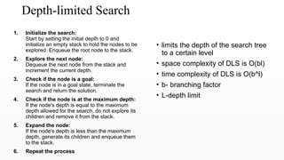
25. Depth-limited Search
1. Initialize the search:
Start by setting the initial depth to 0 and
initialize an empty stack to hold the nodes to be
explored. Enqueue the root node to the stack.
2. Explore the next node:
Dequeue the next node from the stack and
increment the current depth.
3. Check if the node is a goal:
If the node is in a goal state, terminate the
search and return the solution.
4. Check if the node is at the maximum depth:
If the node's depth is equal to the maximum
depth allowed for the search, do not explore its
children and remove it from the stack.
5. Expand the node:
If the node's depth is less than the maximum
depth, generate its children and enqueue them
to the stack.
6. Repeat the process
• limits the depth of the search tree
to a certain level
• space complexity of DLS is O(bl)
• time complexity of DLS is O(b^l)
• b- branching factor
• L-depth limit

26. Bidirectional Search
• to find the shortest path between a source
node and a destination node in a graph
• simultaneously explores the graph from both
the source and destination nodes until they
meet in the middle.
1. Start with the source and destination nodes.
2. Create two search trees:
one from the source node and the other
from the destination node.
3. Expand the search tree from the source
node by generating its child nodes.
4. Expand the search tree from the destination
node by generating child nodes.
5. Check if any node in the search tree
from the source node matches a node
in the search tree from the destination
node.
6. A path between the source and
destination nodes has been found if a
match is found. Return the path.
7. If a match is not found, repeat steps 3-
6 until a match is found or there are no
more nodes to explore.
• Time and space complexity is O(

27. What is shortest path
between A and J?
The branching factor of
this graph is three since
each node has three
neighboring nodes on
average.
Therefore, the distance
between A and J is 5, as
the shortest path is A-B-
C-F-I-J.

28. Key aspects to compare
• Completeness: Guaranteed to find a solution if one exists.
• Optimality: Guaranteed to find the best (e.g., shortest or lowest-
cost) solution.
• Time Complexity: Measures the time taken to find a solution in
terms of the number of nodes visited.
• Space Complexity: Measures the amount of memory required to
store the nodes generated and explored.
• Goal Test: When the algorithm checks if a generated/expanded
node is the goal state.

29. Feature Breadth-First Search (BFS) Depth-First Search (DFS) Depth-Limited Search (DLS) Bidirectional Search
Completen
ess
Yes (if a solution exists)
Yes (if state space is finite, or
if a solution exists and there
are no infinite paths)
Yes (if a solution exists within
the depth limit)
Yes (if BFS is used in both
directions and a solution
exists)
Optimality
Yes (for unweighted
graphs/uniform cost)
No No
Yes (if BFS is used in both
directions and edge costs are
uniform)
Time
Complexity
?
?
(where m is max depth of
state space)
?
(where l is depth limit)
?
Space
Complexity
?
? ? ?
Search
Strategy
Expands shallowest nodes
first
Expands deepest nodes first
Expands deepest nodes first,
up to a limit
Two simultaneous searches
(forward from start, backward
from goal)
Goal Test
When node is generated
(often)
When node is expanded
(often)
When node is expanded
(often)
When a node from one search
meets a node from the other

30. Feature Breadth-First Search (BFS) Depth-First Search (DFS) Depth-Limited Search (DLS) Bidirectional Search
Advantage
s
Finds shortest path in terms of
number of edges; complete.
Low memory requirement
compared to BFS.
Can be more efficient than
DFS if solution is shallow.
Significantly reduces time
complexity in many cases.
Disadvanta
ges
High memory requirement;
can be slow for deep
solutions.
Can get stuck in infinite paths;
not optimal.
Incomplete if solution is
beyond depth limit; finding
good depth limit is hard.
Requires a defined goal state;
can be complex to implement;
requires ability to reverse
operators.
Use Cases
Shortest path problems on
unweighted graphs; finding
direct connections.
When memory is a significant
constraint; when solutions are
expected to be deep.
When there's a known or
estimated depth for the
solution; as a component of
Iterative Deepening DFS.
When both forward and
backward search are feasible
and the branching factor is
high.

31. INFORMED SEARCH
STRATEGIES
use heuristic functions to guide the search
process, leading to more efficient solutions
compared to uninformed search methods

32. Introduction to Search
• - Search in AI = Navigating from start state to goal
• - State space:
• - Nodes = States
• - Edges = Actions
• - Types of search:
• - Uninformed (BFS, DFS)
• - Informed (Heuristic)

33. Uninformed vs Informed Search
• Blind Search : These strategies have
no information about the "goodness" of
a state or how close it is to the goal.
They explore the state space
systematically, without any specific
guidance. Examples include Breadth-
First Search (BFS) and Depth-First
Search (DFS).
• Heuristic Search: Informed search
strategies, unlike their "blind"
counterparts, leverage additional
knowledge about the problem to guide
their search. This knowledge comes
in the form of a heuristic function,
which estimates how "promising" a
state is, or how close it is to the goal.

34. Heuristics in search

35. Key properties of good heuristics:
• Admissibility: A heuristic
h(n) is admissible if, for
every node n, the estimated
cost to reach the goal from n
is never greater than the true
cost to reach the goal from n.
• Consistency (or
Monotonicity): moving from
one state to an adjacent state
should not decrease your
estimated distance to the goal
by more than the actual cost
of that step.
• h(n) > c(n,n′)+h(n′)

36. Greedy Best First Search

37. • Evaluating the cost of each possible path and then expanding the path with the lowest
cost. This process is repeated until the goal is reached.
• The heuristic function takes into account the cost of the current path and the
estimated cost of the remaining paths.
• If the cost of the current path is lower than the estimated cost of the remaining paths,
then the current path is chosen. This process is repeated until the goal is reached.

38. ALGORITHM
• Initialization: Start with the initial state in a "frontier" (priority queue) ordered by the
heuristic value h(n) (estimated cost to goal).
• Expansion:
• Pick the node from the frontier that has the lowest heuristic value h(n). This is the
node the heuristic "thinks" is closest to the goal.
• If this node is the goal, stop.
• Otherwise, generate its successors (neighbors).
• Update Frontier: For each successor, calculate its heuristic value h(n′), and add it to
the frontier.
• Repeat: Continue steps 2 and 3 until the goal is found or the frontier is empty.

39. Advantages & Disadvantages
• Simple and Easy to
Implement
• Fast and Efficient
• Low Memory Requirements
• Flexible
• Efficient with good heuristic
functions
• Inaccurate Results: not always
guaranteed to find the optimal solution
• Local Optima: the path chosen may
not be the best possible path.
• Heuristic Function: a heuristic
function adds complexity to the
algorithm.
• Lack of Completeness: it may not
always find a solution if one exists.
This can happen if the algorithm gets
stuck in a cycle or if the search space
is a too much complex.

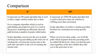
40. A * Algorithm (A-star)
• It combines the best features of Uniform-Cost Search (which is optimal but
uninformed) and Greedy Best-First Search (which is fast but not optimal).
• g(n): The actual cost (or path cost) from the initial state to node n. This is
the cumulative cost of the path found so far to reach n.
• h(n): The estimated cost (heuristic value) from node n to the goal state.

41. ALGORITHM
Step-01:
Define a list OPEN.
Initially, OPEN consists solely of a single node,
the start node S.
Step-02:
If the list is empty, return failure and exit.
Step-03:
Remove node n with the smallest value of f(n)
from OPEN and move it to list CLOSED.
If node n is a goal state, return success and exit.
Step-04:
Expand node n.
Step-05:
If any successor to n is the goal node, return
success and the solution by tracing the path
from goal node to S.
Otherwise, go to Step-06.
Step-06:
For each successor node,
Apply the evaluation function f to the node.
If the node has not been in either list, add it to
OPEN.
Step-07:
Go back to Step-02

42. • The implementation of A* Algorithm involves maintaining two lists- OPEN and CLOSED.
• OPEN contains those nodes that have been evaluated by the heuristic function but have not been
expanded into successors yet.
• CLOSED contains those nodes that have already been visited.
• This systematic approach ensures that A* will always find the optimal path if:
• The heuristic function is admissible (never overestimates)
• A path actually exists between the start and goal nodes
• A* Algorithm maintains a tree of paths originating at the initial state.
• It extends those paths one edge at a time.
• It continues until final state is reached.

43. • Given an initial state of an 8-puzzle problem and final state to be reached-
• Find the most cost-effective path to reach the final state from initial state
using A* Algorithm.
• Consider g(n) = Depth of node and h(n) = Number of misplaced tiles.
SOLUTION

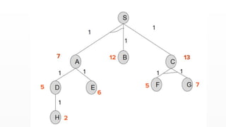
44. Numerical Problem
• Apply A* Search from S to G.
• Trace the path that A* Search would take, showing the
g(n), h(n), and f(n) values for each node as they are put
into the priority queue (frontier).
• What is the total cost of the path found?
h(S)=6 h(D)=2
h(A)=3 h(E)=1
h(B)=5 h(G)=0
h(C)=2

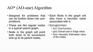
45. AO* (AO-star) Algorithm
• designed for problems that
can be broken down into sub-
problems.
• These are like regular nodes
in a typical search graph.
• Node in the graph will point
both down to its successors
and up to its parent nodes.
• Each Node in the graph will
also have a heuristic value
associated with it.
• f(n)=g(n)+h(n)
• f(n): Cost function.
• g(n): Actual cost or Edge value
• h(n): Heuristic/ Estimated value
of the nodes

46. OR Nodes (Standard Nodes): To solve an
OR node, you need to solve any one of its
successor nodes.
AND Nodes: These nodes represent a
problem that can be decomposed into a set
of sub-problems, all of which must be
solved to solve the parent problem
The algorithm does not explore all the
solution path once it find a solution
The AO* algorithm is not
optimal because it stops as soon as it finds
a solution and does not explore all the
paths.
AO* is complete, meaning it finds a
solution, if there is any, and does not
fall into an infinite loop. Moreover, the AND
feature in this algorithm reduces the
demand for memory.

47. ALGORITHM
1. Initialize the graph to start node
2. Traverse the graph following the current path accumulating nodes that have not
yet been expanded or solved
3. Pick any of these nodes and expand it and if it has no successors call this value
FUTILITY otherwise calculate only f` for each of the successors.
4. If f` is 0 then mark the node as SOLVED
5. Change the value of f` for the newly created node to reflect its successors by
backpropagation.
6. Wherever possible use the most promising routes and if a node is marked as
SOLVED then mark the parent node as SOLVED.
7. If starting node is SOLVED or value greater than FUTILITY, stop, else repeat
from 2.

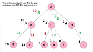
49. Forward Propagation
• First, we begin from node A
and calculate each of the OR
side and AND side paths.
• The OR side path
P(A-B) = G(B) + H(B) = 1 + 5 =
6,
where 1 is the cost of the edge
between A and B,
and 5 is the estimated cost from
B to the goal node.
• The AND side path
• P(A-C-D) = G(C) + H(C) + G(D) +
H(D) = 1 + 3 + 1 + 4 = 9, where
the first 1 is the cost of the edge
between A and C,
• 3 is the estimated cost from C to
the goal node,
• the second 1 is the cost of the
edge between A and D,
• and 4 is the estimated cost from
D to the goal node.

51. Reaching the Last Level and Back Propagation
• In this step we continue on
the P(A-B) from B to its
successor nodes i.e., E and
F, where
• P(B-E) = 1 + 10 = 11 and
• P(B-F) = 1 + 11 = 12.
• Here, P(B-E) has a lower cost
and would be chosen.
• Now, we have reached the bottom
of the graph where no more level
is given to add to our information.
• Therefore, we can do the
backpropagation and correct the
heuristics of upper levels.
• In this side, the updated
• H(B) = P(B-E) = 11, and the
updated
• P(A-B) = G(B) + updated H(B) = 1
+ 11 = 12.

53. Correcting the Path from Start Node
• In this step, we do the
calculations for the AND side
path, i.e.,
P(A-C-D),
• and first explore the paths
attached to node C.
• In this node again we have an
OR side where
• P(C-G) = 1 + 3 = 4, and
• an AND side where
• P(C-H-I) = 1 + 0 + 1 + 0 = 2,
• and as a consequence, the
updated H(C) = 2.
• The updated H(D) = 2, since
• P(D-J) = 1 + 1 = 2.
• By these updated values for
H(C) and H(D), the updated
• P(A-C-D) = 1 + 2 + 1 + 2 = 6.

54. The minimum cost path from A to the goal
node goes from P(A-C-D) by the cost of 6.

57. Comparison

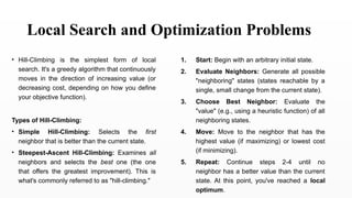
58. Local Search and Optimization Problems
• Hill-Climbing is the simplest form of local
search. It's a greedy algorithm that continuously
moves in the direction of increasing value (or
decreasing cost, depending on how you define
your objective function).
Types of Hill-Climbing:
• Simple Hill-Climbing: Selects the first
neighbor that is better than the current state.
• Steepest-Ascent Hill-Climbing: Examines all
neighbors and selects the best one (the one
that offers the greatest improvement). This is
what's commonly referred to as "hill-climbing."
1. Start: Begin with an arbitrary initial state.
2. Evaluate Neighbors: Generate all possible
"neighboring" states (states reachable by a
single, small change from the current state).
3. Choose Best Neighbor: Evaluate the
"value" (e.g., using a heuristic function) of all
neighboring states.
4. Move: Move to the neighbor that has the
highest value (if maximizing) or lowest cost
(if minimizing).
5. Repeat: Continue steps 2-4 until no
neighbor has a better value than the current
state. At this point, you've reached a local
optimum.

59. Problems with Hill-Climbing
• Local Maxima (or Minima):
If the landscape has multiple
peaks, hill-climbing can get
stuck on a peak that is not the
highest (the global optimum). It
stops when it can't find a better
neighbor, even if a much better
solution exists far away.
• Ridges: A sequence of local
maxima that create a "ridge" might
prevent movement to a higher
peak if the path involves moving
"downhill" temporarily.
• Plateaus: A flat area where all
neighbours have the same value
as the current state, making it
impossible to decide which way to
move.

60. Local-Beam Search
• Local Beam Search is an extension of hill-
climbing that attempts to mitigate the problem
of local maxima by exploring multiple paths in
parallel. Instead of keeping track of just one
current state, it keeps track of k states at any
given time.
• While better than single hill-climbing, it can
still get stuck in areas of the search space if
all k states converge on the same local
optimum.
• The initial random selection of k states is
crucial.
1. Start: Begin with k randomly generated
initial states.
2. Generate Successors: For each of the
k current states, generate all its
successors.
3. Select Best k: From the entire pool of
generated successors (from all k current
states), select the best k unique states
to form the next set of current states.
4. Repeat: Continue steps 2-3 until a goal
state is found or no further improvement
is possible among the k states.

61. Constraint Satisfaction Problems (CSPs)
• Standard search problem -
• state is a "black box“ – any data
structure that supports successor
function, heuristic function, and
goal test
• CSP:
• state is defined by variables Xi
with values from domain Di
• goal test is a set of constraints
specifying allowable combinations
of values for subsets of variables
• Unary constraints involve a
single variable,
• e.g., SA ≠ green
• Binary constraints involve
pairs of variables,
• e.g., SA ≠ WA
• Higher-order constraints
involve 3 or more variables,
• e.g., SA ≠ WA ≠ NT

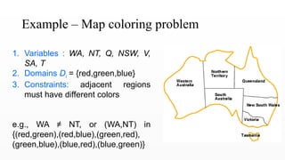
62. Example – Map coloring problem
1. Variables : WA, NT, Q, NSW, V,
SA, T
2. Domains Di = {red,green,blue}
3. Constraints: adjacent regions
must have different colors
e.g., WA ≠ NT, or (WA,NT) in
{(red,green),(red,blue),(green,red),
(green,blue),(blue,red),(blue,green)}

63. Constraint Graph
• Binary CSP: each constraint relates two variables
• Constraint graph: nodes are variables, arcs are constraints

64. Example – Cryptarithmetic Problem
• Each letter or symbol in a mathematical puzzle is uniquely assigned a digit from
0 to 9.
• The goal is to find the correct digit for each letter so that the arithmetic operation
holds true.
Rules:
1. Each letter corresponds to a unique digit, meaning no two letters share the same
number.
2. Digits used range from 0 to 9, covering all possible single-digit numbers.
3. Only one carry-over is allowed during the addition process, which adds a layer of
complexity to the puzzle.
4. The problem can be approached and solved from both the left and right sides, allowing
flexibility in strategy.

65. Solve this-
• S E N D + M O R E = MONEY
• Variables: Letters S, E, N, D,
M, O, R, Y represent digits
• Domains:
• S and M: digits 1–9
• Other letters: digits 0–9
• Constraint 1: Each letter
corresponds to a unique digit
• Constraint 2: Letters S and M
cannot be zero (leading
digits)
• Constraint: All letters must
have different digits

66. Real Life CSPs-
• Timetable Scheduling – which class is to be conducted where?
• Assignment Problems – who teaches what?
• Transportation Scheduling
• Factory Scheduling

67. Standard search formulation (incremental)
• States are defined by the values assigned so far.
• Initial state: the empty assignment, { }
• Successor function: assign a value to an unassigned variable that does not conflict with
current assignment.
• Fail if no legal assignments (not fixable!)
• Goal test: the current assignment is complete
Note:
1. This is the same for all CSPs!
2. Every solution appears at depth n with n variables use depth-first search
⇒
3. Path is irrelevant, so can also use complete-state formulation
4. However, with domain of size d, branching factor b = (n − ℓ)d at depth ℓ, hence n! leaves!

68. Backtracking Search
• Order of variables in variable assignments is irrelevant i.e.,
(WA = r, NT = g) same as (NT = g, WA = r)
• Only need to consider assignments to a single variable at each node⇒ b = d
and there are leaves.
• Depth-first search for CSPs with single-variable assignments is called
backtracking search
• Backtracking search is the basic uninformed algorithm for CSPs
• Can solve n-queens for n ≈ 25

69. Cryptarithmetic Solving by Backtracking
• First, identify all the unique characters from the given
arithmetic expression.
• Next, try assigning digits to the letters. If duplicity is
found backtrack and unassign. This way all possible
combinations of digits for each letter will be generated.
• Now, replace the letters with digits and check if the
expression is true.

70. Map Coloring Solution

72. Completeness & Optimality
• Completeness: Backtracking search is complete. If a solution
exists, it will eventually find it (assuming finite domains and no
infinite loops).
• Optimality: Standard backtracking search finds a solution. If
you want an optimal solution for an optimization problem (COP),
you might need to modify it to find all solutions and pick the
best, or use branch-and-bound techniques.

73. GAME PLAYING
ALGORITHMS
ADVERSARIAL SEARCHES

74. Adversarial Search
• deals with situations where there are multiple agents, and their
goals are in conflict.
• This is the domain of Game Theory within AI.
• Key Concepts to use –
1. Adversarial Search: The process of choosing the best move
for a player in a game where the opponent also plays
optimally to maximize their own utility (and thus minimize
yours).

75. 2. Games in AI Context: In AI, "games" are formalized
situations with:
• Players: Two or more agents.
• States: Configurations of the game
board/environment.
• Moves/Actions: Actions players can take to
transition between states.
• Terminal States: States where the game ends
(win, lose, draw).
• Payoff/Utility Function: A numerical value
assigned to each terminal state, indicating the
desirability of that state for a particular player.
• A positive value for a win, a negative for a loss,
zero for a draw.
3. Zero-Sum Games: A common type of game in
adversarial search. In a zero-sum game, the sum
of the payoffs for all players at the end of the
game is always zero. This means one player's
gain is exactly another player's loss.
4. Game Trees: Adversarial search problems are
often represented using game trees.
• Nodes: Represent game states.
• Edges: Represent moves by a player.
• Levels: Alternate between players (e.g.,
your turn, opponent's turn, your turn, etc.).
• Root Node: The current state of the game.
• Leaf Nodes (Terminal States): Represent
the end of the game, with associated utility
values.

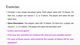
76. Exercise-
• Consider a very simple two-player game. Each player starts with 10 tokens. On
their turn, a player can remove 1, 2, or 3 tokens. The player who takes the last
token wins.
• Game Description: Two players, start with 10 tokens. On their turn, a player can
remove 1, 2, or 3 tokens. The player who takes the last token wins.
• Is this a zero-sum game?
• If it's your turn and there are 4 tokens left, what are your possible moves?
• For each of those moves, what would be the number of tokens left for your
opponent?

77. MinMax Algorithm
• Recursive algorithm used in game theory, artificial intelligence,
and decision theory for two-player, zero-sum games.
• It chooses the next move by assuming that the opponent will
also play optimally to maximize their own score, which in a
zero-sum game means minimizing your score.
• explores the entire game tree from the current state down to a
certain depth (or until terminal states are reached), evaluating
the utility of each terminal state.
• It then propagates these utility values back up the tree, making
optimal choices at each step.

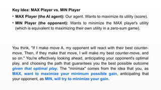
78. Key Idea: MAX Player vs. MIN Player
• MAX Player (the AI agent): Our agent. Wants to maximize its utility (score).
• MIN Player (the opponent): Wants to minimize the MAX player's utility
(which is equivalent to maximizing their own utility in a zero-sum game).
You think, "If I make move A, my opponent will react with their best counter-
move. Then, if they make that move, I will make my best counter-move, and
so on." You're effectively looking ahead, anticipating your opponent's optimal
play, and choosing the path that guarantees you the best possible outcome
given that optimal play. The "minimax" comes from the idea that you, as
MAX, want to maximize your minimum possible gain, anticipating that
your opponent, as MIN, will try to minimize your gain.

79. Algorithm
1. Generate the Game Tree: From the current state, generate all possible future game
states up to a certain depth, or until all terminal states are reached within that depth.
2. Evaluate Terminal Nodes: Assign a utility value (score) to each terminal node from the
perspective of the MAX player.
1. Win for MAX: High positive value (e.g., +10)
2. Loss for MAX: High negative value (e.g., -10)
3. Draw: Zero or a neutral value (e.g., 0)
3. Propagate Values Up the Tree (Recursively):
1. At MAX nodes (It's MAX's turn): The value of a MAX node is the maximum of the utility values of
its children nodes. MAX chooses the move that leads to the state with the highest utility.
2. At MIN nodes (It's MIN's turn): The value of a MIN node is the minimum of the utility values of its
children nodes. MIN chooses the move that leads to the state with the lowest utility (from MAX's
perspective).
4. Determine Optimal Move: The best move for the MAX player from the initial state is the
one that leads to the child node whose value was propagated back up as the maximum.

80. Properties of Minimax
• Completeness: Yes, if the game tree is finite.
• Optimality: Yes, it finds the optimal move assuming the opponent
plays optimally.
• Time Complexity: O(bm), where b is the branching factor
(average number of legal moves from a state) and m is the
maximum depth of the tree.
• This is exponential and becomes prohibitive for games with large
search spaces (like chess).
• Space Complexity: O(bm) for depth-first implementation, O(bm)
for breadth-first.

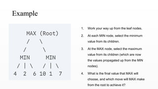
81. Example
1. Work your way up from the leaf nodes.
2. At each MIN node, select the minimum
value from its children.
3. At the MAX node, select the maximum
value from its children (which are now
the values propagated up from the MIN
nodes).
4. What is the final value that MAX will
choose, and which move will MAX make
from the root to achieve it?

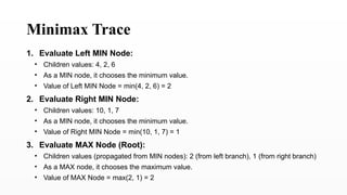
82. Minimax Trace
1. Evaluate Left MIN Node:
• Children values: 4, 2, 6
• As a MIN node, it chooses the minimum value.
• Value of Left MIN Node = min(4, 2, 6) = 2
2. Evaluate Right MIN Node:
• Children values: 10, 1, 7
• As a MIN node, it chooses the minimum value.
• Value of Right MIN Node = min(10, 1, 7) = 1
3. Evaluate MAX Node (Root):
• Children values (propagated from MIN nodes): 2 (from left branch), 1 (from right branch)
• As a MAX node, it chooses the maximum value.
• Value of MAX Node = max(2, 1) = 2

84. Properties & Limitations-
• Deterministic: The outcomes are
predictable, with no randomness
involved.
• Perfect Information: The algorithm
assumes that all players have complete
knowledge of the game.
• Zero-sum: Gains for one player
correspond to losses for the other,
making it ideal for competitive games
like chess​
.
• Depth-first Search: Mini-Max uses a
depth-first search method, exploring the
deepest game states first.
• Computational Complexity: Mini-Max
explores every possible move down to
terminal nodes, which can be
computationally expensive. The number of
evaluations grows exponentially as the game
tree deepens.
• No Probabilistic Handling: Mini-Max is not
suitable for games involving chance
elements, such as dice rolls, since it doesn’t
handle probabilistic events well​
.
• Exponential Time Complexity: The time
complexity of Mini-Max is O(b^d), where ‘b’
is the branching factor and ‘d’ is the depth of
the game tree. This makes it impractical for
games with very large search spaces.

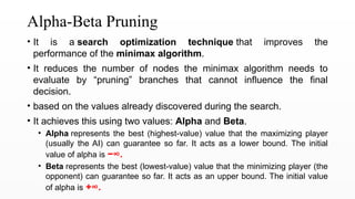
85. Alpha-Beta Pruning
• It is a search optimization technique that improves the
performance of the minimax algorithm.
• It reduces the number of nodes the minimax algorithm needs to
evaluate by “pruning” branches that cannot influence the final
decision.
• based on the values already discovered during the search.
• It achieves this using two values: Alpha and Beta.
• Alpha represents the best (highest-value) value that the maximizing player
(usually the AI) can guarantee so far. It acts as a lower bound. The initial
value of alpha is −∞.
• Beta represents the best (lowest-value) value that the minimizing player (the
opponent) can guarantee so far. It acts as an upper bound. The initial value
of alpha is +∞.

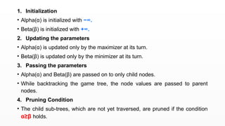
86. 1. Initialization
• Alpha(α) is initialized with −∞.
• Beta(β) is initialized with +∞.
2. Updating the parameters
• Alpha(α) is updated only by the maximizer at its turn.
• Beta(β) is updated only by the minimizer at its turn.
3. Passing the parameters
• Alpha(α) and Beta(β) are passed on to only child nodes.
• While backtracking the game tree, the node values are passed to parent
nodes.
4. Pruning Condition
• The child sub-trees, which are not yet traversed, are pruned if the condition
α≥β holds.

87. Example

88. With
Pruning

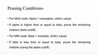
89. Pruning Conditions-
• For MAX node: Alpha = max(alpha, child’s value)
• If alpha is higher than or equal to beta, prune the remaining
children (beta cutoff).
• For MIN node: Beta = min(beta, child’s value)
• If beta is less than or equal to beta, prune the remaining
children (using the alpha cutoff).

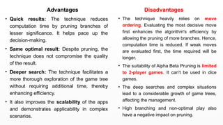
90. Advantages
• Quick results: The technique reduces
computation time by pruning branches of
lesser significance. It helps pace up the
decision-making.
• Same optimal result: Despite pruning, the
technique does not compromise the quality
of the result.
• Deeper search: The technique facilitates a
more thorough exploration of the game tree
without requiring additional time, thereby
enhancing efficiency.
• It also improves the scalability of the apps
and demonstrates applicability in complex
scenarios.
Disadvantages
• The technique heavily relies on move
ordering. Evaluating the most decisive move
first enhances the algorithm's efficiency by
allowing the pruning of more branches. Hence,
computation time is reduced. If weak moves
are evaluated first, the time required will be
longer.
• The suitability of Alpha Beta Pruning is limited
to 2-player games. It can't be used in dice
games.
• The deep searches and complex situations
lead to a considerable growth of game trees,
affecting the management.
• High branching and non-optimal play also
have a negative impact on pruning.

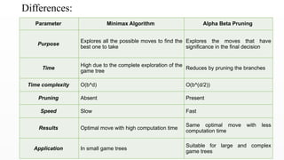
91. Differences:
Parameter Minimax Algorithm Alpha Beta Pruning
Purpose
Explores all the possible moves to find the
best one to take
Explores the moves that have
significance in the final decision
Time
High due to the complete exploration of the
game tree
Reduces by pruning the branches
Time complexity O(b^d) O(b^(d/2))
Pruning Absent Present
Speed Slow Fast
Results Optimal move with high computation time
Same optimal move with less
computation time
Application In small game trees
Suitable for large and complex
game trees