Hshishshsisnshajsjshshs

1. Numpy basics arrays and vectorized computation
UNIT-03

2. INTRODUCTION
• NumPy, short for Numerical Python, has long been a cornerstone of numerical computing in Python.
• NumPy is a basic package for scientific computing with Python and especially for data analysis.
NumPy contains, among other things:
• A fast and efficient multidimensional array object ndarray.
• Functions for performing element-wise computations with arrays or mathematical operations between arrays
• Tools for reading and writing array-based datasets to disk
• Linear algebra operations, Fourier transform, and random number generation
• A mature C API to enable Python extensions and native C or C++ code to access NumPy’s data structures and
computational facilities.
• one of its primary uses in data analysis is as a container for data to be passed between algorithms and
libraries.

3. INTRODUCTION
• One of the reasons NumPy is so important for numerical computations in Python is because it is designed for
efficiency on large arrays of data. There are a number of reasons for this:
1. NumPy internally stores data in a contiguous block of memory, independent of other built-in Python objects.
NumPy’s library of algorithms written in the C language can operate on this memory without any type
checking or other overhead. NumPy arrays also use much less memory than built-in Python sequences.
2. NumPy operations perform complex computations on entire arrays without the need for Python for loops.

5. The NumPy ndarray:
A multidimensional array object
• One of the key features of NumPy is its N-dimensional array object, or ndarray, which is a fast, flexible container for large datasets in
Python. Arrays enable you to perform mathematical operations on whole blocks of data using similar syntax to the equivalent
operations between scalar elements.
• To give you a flavor of how NumPy enables batch computations with similar syntax to scalar values on built-in Python objects, I first
import NumPy and generate a small array of random data:
• In [12]: import numpy as np
• # Generate some random data
• In [13]: data = np.random.randn(2, 3)
• In [14]: data
• Out[14]:
• array([[-0.2047, 0.4789, -0.5194],
• [-0.5557, 1.9658, 1.3934]])

6. In [16]: data + data
Out[16]:array([[-0.4094, 0.9579, -1.0389], [-1.1115, 3.9316, 2.7868]])
In the first example, all of the elements have been multiplied by 10. In the second, the
corresponding values in each “cell” in the array have been added to each other.

7. First import NumPy and generate a small array of random data:
In [12]: import numpy as np
# Generate some random data
In [13]: data = np.random.randn(2, 3)
In [14]: data
Out[14]:
array([[-0.2047, 0.4789, -0.5194],
[-0.5557, 1.9658, 1.3934]])
I then write mathematical operations
with data:
In [15]: data * 10
Out[15]:
array([[ -2.0471, 4.7894, -5.1944],
[ -5.5573, 19.6578, 13.9341]])
In [16]: data + data
Out[16]:
array([[-0.4094, 0.9579, -1.0389],
[-1.1115, 3.9316, 2.7868]])
An ndarray is a generic multidimensional
container for homogeneous data; that is,
all
of the elements must be the same type.
Every array has a shape, a tuple indicating
the size of each dimension, and a dtype,
an object describing the data type of the
array:
In [17]: data.shape
Out[17]: (2, 3)
In [18]: data.dtype
Out[18]: dtype('float64')

8. The NumPy ndarray:
A multidimensional array object
• An ndarray is a generic multidimensional container for homogeneous data; that is, all of the
elements must be the same type.
• Every array has a shape, a tuple indicating the size of each dimension, and a dtype, an object
describing the data type of the array:
• >>> a = np.array([1, 2, 3])
• >>> a
• array([1, 2, 3])
• >>> type(a)
• <type 'numpy.ndarray'>

9. • In order to know the associated dtype to the just created ndarray, you have to use the dtype attribute.
• The data type is stored in a special dtype metadata object
• >>> a.dtype
• dtype('int32')
• >>> a.ndim
• 1
• >>> a.size
• 3
The NumPy ndarray:
A multidimensional array object

10. Creating ndarrays
• To define a new ndarray, the easiest way is to use the array() function, passing a Python list containing the elements to be included in it
as an argument.
• Example:
• In [19]: data1 = [6, 7.5, 8, 0, 1]
• In [20]: arr1 = np.array(data1)
• In [21]: arr1
• Out[21]: array([ 6. , 7.5, 8. , 0. , 1. ])
• But the use of arrays can be easily extended to the case with several dimensions. For example, if you define a two-dimensional array 2x2:
• >>> b = np.array([[1.3, 2.4],[0.3, 4.1]])
• >>> b.dtype
• dtype('float64')
• >>> b.ndim
• 2
• >>> b.size
• 4
• >>> b.shape
• (2L, 2L)
• This array has rank 2, since it has two axis, each of length 2.

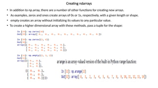
11. • In addition to np.array, there are a number of other functions for creating new arrays.
• As examples, zeros and ones create arrays of 0s or 1s, respectively, with a given length or shape.
• empty creates an array without initializing its values to any particular value.
• To create a higher dimensional array with these methods, pass a tuple for the shape:
Creating ndarrays

12. • In [25]: np.empty((2, 3, 2))
• Out[25]:
• array([[[ 4.94065646e-324, 4.94065646e-324],
• [ 3.87491056e-297, 2.46845796e-130],
• [ 4.94065646e-324, 4.94065646e-324]],
• [[ 1.90723115e+083, 5.73293533e-053],
• [ -2.33568637e+124, -6.70608105e-012],
• [ 4.42786966e+160, 1.27100354e+025]]])

14. Data Types for ndarrays
• The data type or dtype is a special object containing the information (or metadata, data about data) the ndarray needs to
interpret a chunk of memory as a particular type of data:
• In [33]: arr1 = np.array([1, 2, 3], dtype=np.float64)
• In [34]: arr2 = np.array([1, 2, 3], dtype=np.int32)
• In [35]: arr1.dtype
• Out[35]: dtype('float64')
• Additionally NumPy provides types of its own. numpy.int32, numpy.int16, and numpy.float64 are some examples.
• dtypes are a source of NumPy’s flexibility for interacting with data coming from other systems.
• The numerical dtypes are named the same way: a type name, like float or int, followed by a number indicating the number of
bits per element.
• A standard doubleprecision floating-point value (what’s used under the hood in Python’s float object) takes up 8 bytes or 64
bits. Thus, this type is known in NumPy as float64.

15. • The type of the array can also be explicitly specified at creation time:
• >>>c = np.array([[1, 2], [3, 4]], dtype=complex)
• >>>c
• >>>array([[1.+0.j, 2.+0.j],
• [3.+0.j, 4.+0.j]])
Data Types for ndarrays

17. • You can explicitly convert or cast an array from one dtype to another using ndarray’s astype
method:
• In [37]: arr = np.array([1, 2, 3, 4, 5])
• In [38]: arr.dtype
• Out[38]: dtype('int64')
• In [39]: float_arr = arr.astype(np.float64)
• In [40]: float_arr.dtype
• Out[40]: dtype('float64')
Data Types for ndarrays

18. • In this example, integers were cast to floating point. If I cast some floating-point numbers
to be of integer dtype, the decimal part will be truncated:
• In [41]: arr = np.array([3.7, -1.2, -2.6, 0.5, 12.9, 10.1])
• In [42]: arr
• Out[42]: array([ 3.7, -1.2, -2.6, 0.5, 12.9, 10.1])
• In [43]: arr.astype(np.int32)
• Out[43]: array([ 3, -1, -2, 0, 12, 10], dtype=int32)
Data Types for ndarrays

19. • If you have an array of strings representing numbers, you can use astype to
convert them to numeric form:
• In [44]: numeric_strings = np.array(['1.25', '-9.6', '42'], dtype=np.string_)
• In [45]: numeric_strings.astype(float)
• Out[45]: array([ 1.25, -9.6 , 42. ])
Data Types for ndarrays

20. Printing Arrays
• When you print an array, NumPy displays it in a similar way to nested lists, but with the
following layout:
• the last axis is printed from left to right,
• the second-to-last is printed from top to bottom,
• the rest are also printed from top to bottom, with each slice separated from the next by
an empty line.
• One-dimensional arrays are then printed as rows, bidimensionals as matrices and
tridimensionals as lists of matrices.

21. • >>>a = np.arange(6) # 1d array
• >>>print(a)
• [0 1 2 3 4 5]
• >>>b = np.arange(12).reshape(4, 3) # 2d array
• >>>print(b)
• [[ 0 1 2]
• [ 3 4 5]
• [ 6 7 8]
• [ 9 10 11]]
• >>>c = np.arange(24).reshape(2, 3, 4) # 3d array
• >>>print(c)
• [[[ 0 1 2 3]
• [ 4 5 6 7]
• [ 8 9 10 11]]
• [[12 13 14 15]
• [16 17 18 19]
• [20 21 22 23]]]

22. Arithmetic with NumPy Arrays
• Arrays are important because they enable you to express batch operations on data without writing any for loops. NumPy users
call this vectorization. Any arithmetic operations between equal-size arrays applies the operation element-wise:
• >>>a = np.array([20, 30, 40, 50])
• >>>b = np.arange(4)
• >>>b
• >>>array([0, 1, 2, 3])
• >>>c = a - b
• >>>c
• >>>array([20, 29, 38, 47])
• >>>b**2
• >>>array([0, 1, 4, 9])
• >>>10 * np.sin(a)
• >>>array([ 9.12945251, -9.88031624, 7.4511316 , -2.62374854])
• >>>a < 35
• array([ True, True, False, False])

23. • In [51]: arr = np.array([[1., 2., 3.], [4., 5., 6.]])
• In [52]: arr
• Out[52]:array([[ 1., 2., 3.],
• [ 4., 5., 6.]])
• In [53]: arr * arr
• Out[53]:array([[ 1., 4., 9.],
• [ 16., 25., 36.]])
• In [54]: arr - arr
• Out[54]: array([[ 0., 0., 0.],
• [ 0., 0., 0.]])
Arithmetic with NumPy Arrays

24. • Comparisons between arrays of the same size yield boolean arrays:
• In [57]: arr2 = np.array([[0., 4., 1.], [7., 2., 12.]])
• In [58]: arr2
• Out[58]:
• array([[ 0., 4., 1.],
• [ 7., 2., 12.]])
• In [59]: arr2 > arr
• Out[59]:
• array([[False, True, False],
• [ True, False, True]], dtype=bool)
• Operations between differently sized arrays is called broadcasting.
Arithmetic with NumPy Arrays

25. Basic Indexing and Slicing
• NumPy array indexing is a rich topic, as there are many ways you may want to select a subset of your data
or individual elements. One-dimensional arrays are simple:
• In [60]: arr = np.arange(10)
• In [61]: arr
• Out[61]: array([0, 1, 2, 3, 4, 5, 6, 7, 8, 9])
• In [62]: arr[5]
• Out[62]: 5
• In [63]: arr[5:8]
• Out[63]: array([5, 6, 7])
• In [64]: arr[5:8] = 12
• In [65]: arr
• Out[65]: array([ 0, 1, 2, 3, 4, 12, 12, 12, 8, 9])

26. Fancy Indexing
• Fancy indexing is a term adopted by NumPy to
describe indexing using integer arrays.
• Suppose we had an 8 × 4 array:
• In [117]: arr = np.empty((8, 4))
• In [118]: for i in range(8):
• .....: arr[i] = i
• In [119]: arr
• Out[119]:
• array([[ 0., 0., 0., 0.],
• [ 1., 1., 1., 1.],
• [ 2., 2., 2., 2.],
• [ 3., 3., 3., 3.],
• [ 4., 4., 4., 4.],
• [ 5., 5., 5., 5.],
• [ 6., 6., 6., 6.],
• [ 7., 7., 7., 7.]])
• To select out a subset of the rows in a particular order,
you can simply pass a list or
• ndarray of integers specifying the desired order:
• In [120]: arr[[4, 3, 0, 6]]
• Out[120]:
• array([[ 4., 4., 4., 4.],
• [ 3., 3., 3., 3.],
• [ 0., 0., 0., 0.],
• [ 6., 6., 6., 6.]])
• Using negative indices selects rows from the end:
• In [121]: arr[[-3, -5, -7]]
• Out[121]:
• array([[ 5., 5., 5., 5.],
• [ 3., 3., 3., 3.],
• [ 1., 1., 1., 1.]])

27. • Passing multiple index arrays does something slightly different; it selects a one dimensional array of elements
corresponding to each tuple of indices:
• In [122]: arr = np.arange(32).reshape((8, 4))
• In [123]: arr
• Out[123]:
• array([[ 0, 1, 2, 3],
• [ 4, 5, 6, 7],
• [ 8, 9, 10, 11],
• [12, 13, 14, 15],
• [16, 17, 18, 19],
• [20, 21, 22, 23],
• [24, 25, 26, 27],
• [28, 29, 30, 31]])
• In [124]: arr[[1, 5, 7, 2], [0, 3, 1, 2]]
• Out[124]: array([ 4, 23, 29, 10])
• Here the elements (1, 0), (5, 3), (7, 1), and (2, 2) were selected. Regardless of how many dimensions the array has
(here, only 2), the result of fancy indexing is always one-dimensional.
Fancy Indexing
Here the red color
elements represents
the position ,0,3,1,2
location elements will
be fetched from 1,5,7,2
rows

28. • The behavior of fancy indexing in this case is a bit different from what some users might have expected
(myself included), which is the rectangular region formed by selecting a subset of the matrix’s rows and
columns. Here is one way to get that:
• In [125]: arr[[1, 5, 7, 2]][:, [0, 3, 1, 2]]
• Out[125]:
• array([[ 4, 7, 5, 6],
• [20, 23, 21, 22],
• [28, 31, 29, 30],
• [ 8, 11, 9, 10]])
• Keep in mind that fancy indexing, unlike slicing, always copies the data into a new array.
Fancy Indexing
Red color numbers indicates the
position which means the new
elements will be arranged in this
format

29. Transposing Arrays and Swapping Axes
• Transposing is a special form of reshaping that similarly returns a view on the underlying data without copying
anything.
• Arrays have the transpose method and also the special T attribute:
• In [126]: arr = np.arange(15).reshape((3, 5))
• In [127]: arr
• Out[127]:
• array([[ 0, 1, 2, 3, 4],
• [ 5, 6, 7, 8, 9],
• [10, 11, 12, 13, 14]])
• In [128]: arr.T
• Out[128]:
• array([[ 0, 5, 10],
• [ 1, 6, 11],
• [ 2, 7, 12],
• [ 3, 8, 13],
• [ 4, 9, 14]])

30. • Simple transposing with .T is a special case of swapping axes.
• ndarray has the method swapaxes, which takes a pair of axis numbers and switches the indicated axes to rearrange the data:
• In [135]: arr
• Out[135]:
• array([[[ 0, 1, 2, 3],
• [ 4, 5, 6, 7]],
• [[ 8, 9, 10, 11],
• [12, 13, 14, 15]]])
• In [136]: arr.swapaxes(1, 2)
• Out[136]:
• array([[[ 0, 4],
• [ 1, 5],
• [ 2, 6],
• [ 3, 7]],
• [[ 8, 12],
• [ 9, 13],
• [10, 14],
• [11, 15]]])
Transposing Arrays and Swapping Axes
swapaxes similarly returns a view on the data without making a copy..

31. Universal Functions: Fast Element-Wise Array
Functions
• A universal function, or ufunc, is a function that performs element-wise operations on data in ndarrays.
• You can think of them as fast vectorized wrappers for simple functions that take one or more scalar values
and produce one or more scalar results.
• Many ufuncs are simple element-wise transformations, like sqrt or exp:
• In [137]: arr = np.arange(10)
• In [138]: arr
• Out[138]: array([0, 1, 2, 3, 4, 5, 6, 7, 8, 9])
• In [139]: np.sqrt(arr)
• Out[139]:
• array([ 0. , 1. , 1.4142, 1.7321, 2. , 2.2361, 2.4495,
• 2.6458, 2.8284, 3. ])
• In [140]: np.exp(arr)
• Out[140]:
• array([ 1. , 2.7183, 7.3891, 20.0855, 54.5982,
• 148.4132, 403.4288, 1096.6332, 2980.958 , 8103.0839])
These are referred to as unary ufuncs.

32. • Others, such as add or maximum, take two arrays (thus, binary ufuncs) and return a single array as the result:
• In [141]: x = np.random.randn(8)
• In [142]: y = np.random.randn(8)
• In [143]: x
• Out[143]:
• array([-0.0119, 1.0048, 1.3272, -0.9193, -1.5491, 0.0222, 0.7584,
• -0.6605])
• In [144]: y
• Out[144]:
• array([ 0.8626, -0.01 , 0.05 , 0.6702, 0.853 , -0.9559, -0.0235,
• -2.3042])
• In [145]: np.maximum(x, y)
• Out[145]:
• array([ 0.8626, 1.0048, 1.3272, 0.6702, 0.853 , 0.0222, 0.7584,
• -0.6605])
Universal Functions: Fast Element-Wise Array
Functions

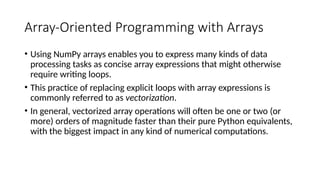
35. Array-Oriented Programming with Arrays
• Using NumPy arrays enables you to express many kinds of data
processing tasks as concise array expressions that might otherwise
require writing loops.
• This practice of replacing explicit loops with array expressions is
commonly referred to as vectorization.
• In general, vectorized array operations will often be one or two (or
more) orders of magnitude faster than their pure Python equivalents,
with the biggest impact in any kind of numerical computations.

36. • As a simple example, suppose we wished to evaluate the function
sqrt(x^2 + y^2) across a regular grid of values.
• The np.meshgrid function takes two 1D arrays and produces two 2D
matrices corresponding to all pairs of (x, y) in the two arrays:
In [155]: points = np.arange(-5, 5, 0.01) # 1000 equally
spaced points
In [156]: xs, ys = np.meshgrid(points, points)
In [157]: ys
Out[157]:
array([[-5. , -5. , -5. , ..., -5. , -5. , -5. ],
[-4.99, -4.99, -4.99, ..., -4.99, -4.99, -4.99],
[-4.98, -4.98, -4.98, ..., -4.98, -4.98, -4.98],
...,
[ 4.97, 4.97, 4.97, ..., 4.97, 4.97, 4.97],
[ 4.98, 4.98, 4.98, ..., 4.98, 4.98, 4.98],
[ 4.99, 4.99, 4.99, ..., 4.99, 4.99, 4.99]])

37. • Now, evaluating the function is a matter of writing the same
expression you would write with two points:
In [158]: z = np.sqrt(xs ** 2 + ys ** 2)
In [159]: z
Out[159]:
array([[ 7.0711, 7.064 , 7.0569, ..., 7.0499, 7.0569,
7.064 ],
[ 7.064 , 7.0569, 7.0499, ..., 7.0428, 7.0499, 7.0569],
[ 7.0569, 7.0499, 7.0428, ..., 7.0357, 7.0428, 7.0499],
...,
[ 7.0499, 7.0428, 7.0357, ..., 7.0286, 7.0357, 7.0428],
[ 7.0569, 7.0499, 7.0428, ..., 7.0357, 7.0428, 7.0499],
[ 7.064 , 7.0569, 7.0499, ..., 7.0428, 7.0499, 7.0569]])

38. • In [160]: import matplotlib.pyplot as plt
• In [161]: plt.imshow(z, cmap=plt.cm.gray);
plt.colorbar()
• Out[161]: <matplotlib.colorbar.Colorbar at
0x7f715e3fa630>
• In [162]: plt.title("Image plot of $sqrt{x^2 +
y^2}$ for a grid of values")
• Out[162]: <matplotlib.text.Text at
0x7f715d2de748>
See Figure 4-3. Here I used the matplotlib
function imshow to create an image plot
from a two-dimensional array of function
values.

39. Expressing Conditional Logic as Array
Operations
• The numpy.where function is a vectorized version of the ternary
expression x if condition else y. Suppose we had a boolean array and
two arrays of values:
In [165]: xarr = np.array([1.1, 1.2, 1.3, 1.4, 1.5])
In [166]: yarr = np.array([2.1, 2.2, 2.3, 2.4, 2.5])
In [167]: cond = np.array([True, False, True, True,
False])

40. Suppose we wanted to take a value from xarr whenever the corresponding value in
cond is True, and otherwise take the value from yarr. A list comprehension doing
this might look like:
In [168]: result = [(x if c else y)
.....: for x, y, c in zip(xarr, yarr, cond)]
In [169]: result
Out[169]: [1.1000000000000001, 2.2000000000000002, 1.3, 1.3999999999999999, 2.5]
This has multiple problems. First, it will not be very fast for large arrays (because all
the work is being done in interpreted Python code). Second, it will not work with
multidimensional arrays. With np.where you can write this very concisely:
In [170]: result = np.where(cond, xarr, yarr)
In [171]: result
Out[171]: array([ 1.1, 2.2, 1.3, 1.4, 2.5])

41. • The second and third
arguments to np.where don’t
need to be arrays; one or
both of them can be scalars.
• A typical use of where in data
analysis is to produce a new
array of values based on
another array.
• Suppose you had a matrix of
randomly generate data and
you wanted to replace all
positive values with 2 and all
negative values with –2. This
is very easy to do with
np.where:
In [172]: arr = np.random.randn(4, 4)
In [173]: arr
Out[173]:
array([[-0.5031, -0.6223, -0.9212, -
0.7262],
[ 0.2229, 0.0513, -1.1577, 0.8167],
[ 0.4336, 1.0107, 1.8249, -0.9975],
[ 0.8506, -0.1316, 0.9124, 0.1882]])
In [174]: arr > 0
Out[174]:
array([[False, False, False, False],
[ True, True, False, True],
[ True, True, True, False],
[ True, False, True, True]], dtype=bool)
In [175]: np.where(arr > 0, 2, -2)
Out[175]:
array([[-2, -2, -2, -2],
[ 2, 2, -2, 2],

42. [ 2, 2, 2, -2],
[ 2, -2, 2, 2]])
You can combine scalars and arrays when using np.where. For example, I
can replace
all positive values in arr with the constant 2 like so:
In [176]: np.where(arr > 0, 2, arr) # set only positive values to 2
Out[176]:
array([[-0.5031, -0.6223, -0.9212, -0.7262],
[ 2. , 2. , -1.1577, 2. ],
[ 2. , 2. , 2. , -0.9975],
[ 2. , -0.1316, 2. , 2. ]])
The arrays passed to np.where can be more than just equal-sized arrays or
scalars.

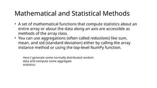
43. Mathematical and Statistical Methods
• A set of mathematical functions that compute statistics about an
entire array or about the data along an axis are accessible as
methods of the array class.
• You can use aggregations (often called reductions) like sum,
mean, and std (standard deviation) either by calling the array
instance method or using the top-level NumPy function.
Here I generate some normally distributed random
data and compute some aggregate
statistics:

44. In [177]: arr = np.random.randn(5, 4)
In [178]: arr
Out[178]:
array([[ 2.1695, -0.1149, 2.0037, 0.0296],
[ 0.7953, 0.1181, -0.7485, 0.585 ],
[ 0.1527, -1.5657, -0.5625, -0.0327],
[-0.929 , -0.4826, -0.0363, 1.0954],
[ 0.9809, -0.5895, 1.5817, -0.5287]])
In [179]: arr.mean()
Out[179]: 0.19607051119998253
In [180]: np.mean(arr)
Out[180]: 0.19607051119998253
In [181]: arr.sum()
Out[181]: 3.9214102239996507
Functions like mean and sum take an optional axis
argument that computes the statistic
over the given axis, resulting in an array with one
fewer dimension
In [182]: arr.mean(axis=1)
Out[182]: array([ 1.022 , 0.1875, -0.502 , -
0.0881, 0.3611])
In [183]: arr.sum(axis=0)
Out[183]: array([ 3.1693, -2.6345, 2.2381,
1.1486])

45. Here, arr.mean(1) means “compute mean across the columns” where
arr.sum(0)
means “compute sum down the rows.”
Other methods like cumsum and cumprod do not aggregate, instead
producing an array
of the intermediate results:
In [184]: arr = np.array([0, 1, 2, 3, 4, 5, 6, 7])
In [185]: arr.cumsum()
Out[185]: array([ 0, 1, 3, 6, 10, 15, 21, 28])
In multidimensional arrays, accumulation functions like cumsum return an
array of
the same size, but with the partial aggregates computed along the indicated
axis
according to each lower dimensional slice:
In [186]: arr = np.array([[0, 1, 2], [3, 4, 5], [6, 7, 8]])
In [187]: arr
Out[187]:
array([[0, 1, 2],
[3, 4, 5],
In [188]: arr.cumsum(axis=0)
Out[188]:
array([[ 0, 1, 2],
[ 3, 5, 7],
[ 9, 12, 15]])
In [189]: arr.cumprod(axis=1)
Out[189]:
array([[ 0, 0, 0],
[ 3, 12, 60],
[ 6, 42, 336]])

46. Table 4-5. Basic array statistical methods

47. Methods for Boolean Arrays
Boolean values are coerced to 1 (True) and 0 (False) in the preceding methods.
Thus,
sum is often used as a means of counting True values in a boolean array:
In [190]: arr = np.random.randn(100)
In [191]: (arr > 0).sum() # Number of positive values
Out[191]: 42
There are two additional methods, any and all, useful especially for boolean arrays.
any tests whether one or more values in an array is True, while all checks if every
value is True:
In [192]: bools = np.array([False, False, True, False])
In [193]: bools.any()
Out[193]: True
In [194]: bools.all()
Out[194]: False
These methods also work with non-boolean arrays, where non-zero elements
evaluate
to True.

48. Sorting
Like Python’s built-in list type, NumPy arrays can be sorted in-place with the sort
method:
In [195]: arr = np.random.randn(6)
In [196]: arr
Out[196]: array([ 0.6095, -0.4938, 1.24 , -0.1357, 1.43 , -0.8469])
In [197]: arr.sort()
In [198]: arr
Out[198]: array([-0.8469, -0.4938, -0.1357, 0.6095, 1.24 , 1.43 ])
You can sort each one-dimensional section of values in a multidimensional array
inplace
along an axis by passing the axis number to sort:
In [199]: arr = np.random.randn(5, 3)
In [200]: arr
Out[200]:
array([[ 0.6033, 1.2636, -0.2555],
[-0.4457, 0.4684, -0.9616],
[-1.8245, 0.6254, 1.0229],
[ 1.1074, 0.0909, -0.3501],
[ 0.218 , -0.8948, -1.7415]])

49. In [201]: arr.sort(1)
In [202]: arr
Out[202]:
array([[-0.2555, 0.6033, 1.2636],
[-0.9616, -0.4457, 0.4684],
[-1.8245, 0.6254, 1.0229],
[-0.3501, 0.0909, 1.1074],
[-1.7415, -0.8948, 0.218 ]])
The top-level method np.sort returns a sorted copy of an array instead
of modifying
the array in-place. A quick-and-dirty way to compute the quantiles of
an array is to
sort it and select the value at a particular rank:
In [203]: large_arr = np.random.randn(1000)
In [204]: large_arr.sort()
In [205]: large_arr[int(0.05 * len(large_arr))] # 5% quantile
Out[205]: -1.5311513550102103