Unit 001Stats (1).pdf

Unit 01.
“Introduction to Statistics”

Contents:
• Definition & History of Statistics
• Scope in different areas
• Population & Sample
• Methods of Sampling and
• Data Condensation & Graphical Methods

Definition & History of Statistics
➢ The subject of Statistics, as it seems, is not a new
discipline but it is as old as the human society
itself.
➢Its origin can be traced to the old days when it
was regarded as the ‘science of State-craft’ and
was the by-product of administrative activity of
the Sate.
➢ The word ‘Statistics’ seems to have been derived
from the Latin word ‘status’ or the Italian word
‘statista’ or the German word ‘statistik’ each of
which means a ‘political state’.

Acharya Vishnugupta Chanakya (Kautilya)
➢In India, an efficient system of collecting official and
administrative statistics existed even more than
2,000 years ago, in particular, during the reign of
Chandra Gupta Maurya (324-300 B.C.).
➢ From Kautilya’s ‘Arthshastra’ it is known that even
before 300 B.C. a very good system of collecting
‘Vital Statistics’ and registration of births and
deaths was in vogue.

King Akbar Raja Todarmal
➢During Akbar’s reign (1556-1605 A.D.), Raja
Todarmal, the then land and revenue minister,
maintained good records of land and agricultural
statistics.
➢In “Aina-e-Akbari” written by Abul Fazl
(in 1596-97), one of the nine gems of Akbar, we
find the detailed accounts of the administrative &
statistical surveys conducted during Akbar’s reign.

Adolf Hitler
➢In Germany, the systematic collection of official
statistics originated towards the end of 18th century
when, in order to have an idea of the relative
strength of different German States, information
regarding population and output – industrial &
agricultural – was collected.

➢In England, statistics were the outcome of
Napoleonic wars. The wars necessitated the
systematic collection of numerical data to enable
the government to assess the revenues and
expenditures with greater precision and then to
levy new taxes in order to meet the cost of war.

Captain John Grant
➢Seventeenth century saw the origin of the ‘Vital
Statistics’. Captain John Grant of London (1620-1674),
known as the ‘father’ of Vital Statistics, was the first
man to study the statistics of births and deaths.
➢ To name the few the following are the giants who
contributed towards modern statistics (what we have
today) which is based on probability concept.

Casper Newman Sir William Petty James Dodson (1623-1687) Dr. Price
Contributed towards concept of Insurance.

Pascal(1623-1662) P. Fermat(1601-1665) James Bernoulli (1654-1705)
De-Moivre (1667-1754) Laplace (1749-1827) Gauss(1777-1855)
Theory of Probability, Principle of Least squares & Normal
Law of Errors.

Sir R. A. Fisher Francis Galton Karl Pearson
W. S. Gosset Pascal(1623-1662) James Bernoulli (1654-1705)
Mathematicians & Statisticians from 18th, 19th & 20th centuries contributed
towards Modern theory of Probability, Regression Analysis, Correlation
Analysis, Probability & exact sampling distributions, theory of estimation,
testing of hypothesis etc.

P. V. Sukhatme R. C. Bose Panse
C.R. Rao Parthasarthy

Definition of Statistics
By some giants
A) Statistics as numerical data:

Webster
“Statistics are the classified facts representing the
conditions of the people in a state… specially those
facts which can be stated in number or in tables of
numbers or in any tabular or classified arrangement.”

Bowley
➢ “Statistics are numerical statement of facts in any department
of enquiry placed in relation to each other.”
➢
Yule Kendall
“By statistics wel mean quantitative data affected to a
marked extent by multiplicity of causes.”

A. M. Tuttle
➢“Statistics are measurements, enumerations or
estimates of natural phenomenon, usually
systematically arranged, analyzed and presented as to
exhibit important inter-relationships among them.” --
➢ “Statistics may be defined as the aggregate of facts to a
marked extent by multiplicity of causes, numerically
expressed, enumerated or estimated according to a
reasonable standard of accuracy, collected in a
systematic manner, for a predetermined purpose and
placed in relation to each other.” -- Prof. Horace Secrist.

B) Statistics as Statistical Methods
➢ Statistics may be called as science of counting.
➢ Statistics may be rightly called the science of
averages. -- Bowley A. L.
➢ Statistics is the science of estimates and
probabilities. -- Boddington.
➢ “Statistics is the science and art of handling
aggregate of facts – observing, enumeration,
recording classifying and otherwise systematically
treating them.” -- Harlow.

Scope of Statistics
in
➢Economics
➢Management Sciences
and
➢Industry

Scope of Statistics in Economics:
➢ Statistical data and technique of statistical analysis
have proved immensely useful in solving a variety of
economic problems, such as wages, prices,
consumption, production, distribution of income
and wealth etc.
➢ Statistical tool like Index numbers, Time series
Analysis, Demand Analysis and Forecasting
Techniques are extensively used for efficient
planning and economic development of a country.

➢ Empirical studies based on sound statistical analysis
have led to the formulation of many economic lows.
For example:
i. ‘Engel’s Law of Consumption’, (1895) was based on
detailed and systematic studies of family budgets
of a number of families.
ii. ‘Pereto’s Law of Income Distribution’ is based on
the empirical study of the income data of different
countries of the world at different times.
iii. Empirical studies based on the observation of the
actual behavior of the buyers in the market led
‘Revealed Preference Analysis’ of Prof. Samuelson.

➢The extensive use of Mathematics & Statistics in the
study of economics have led to the development of
new disciplines called Economic Statistics and
Econometrics.
➢ These days, advance statistical techniques are
used to fit the economic models for obtaining
optimum results subject to a number of constraints
on the resources like capital, labor, production
capacity etc.

Scope of Statistics in Management Sciences
➢ Statistical tools & techniques are widely used
in decision making. For efficient working of different
work areas viz. marketing, sales, production,
logistics, inventory, etc.
➢ Index numbers, Time series Analysis,
Forecasting, SQC, etc statistical tools are important
regarding decision making.
➢ Correlation and Regression Analysis are such
techniques which are vital regarding decision
making.

Scope of Statistics in Management Sciences
➢ Along with these Linear Programming,
Transportation Problems, Sequencing, PERT & CPM,
Assignment Problems, Inventory control are few
optimization techniques to find the optimum
solution.

Scope of Statistics in Industry:
➢In Industry, Statistics is extensively used in ‘Quality
Control’. The main objective in any production
process is to control the quality of the
manufactured product so that it conforms to
specifications. This is called ‘process control’ and is
achieved through the powerful technique of control
charts and inspection plans.

Scope of Statistics in Industry:
Dr. W. A. Shewhart
The discovery of the control charts was made by a young
physicist Dr. W. A. Shewhart of the Bell Telephone
Laboratories (U.S.A.) in 1924 and is based on setting ‘3σ’
(3-sigma) control limits which has its basis on the theory
of probability & normal distribution.

Now a days ‘6σ’ control limits are widely used where
chance of error is almost negligible.
Inspection plans are based on special kind of sampling
techniques which are very important aspect of
statistical theory.

Population
Population in general means number of living persons
in a particular geographical area on a particular time.
It is the usual meaning and is used as population of a
country.

With reference to statistics, meaning of population is
broader sense. Here it means ‘Each and every’, or ‘all’.
The meaning is ‘each and every unit’ which covers
under a given problem is called ‘statistical population’.

Definition:
➢The group of individuals under study is called
‘population’ or ‘universe’.
➢An aggregate of objects or individuals under
study is called “Population or Universe”.
➢Population may contain finite or infinite
elements. Accordingly, it is called as ‘finite or
infinite population’.
➢e.g. Total number of people living in a country,
Total number of students in a college, Total
number of buses with PMT, etc.

Sample
➢“Any part of population or fraction of
population under study is known as
sample”.
➢A finite subset of statistical individuals in a
population is called ‘sample’ and the
number of individuals in a sample is called
the ‘sample size’.

➢In a production process say out of 100
items manufactured & 10 are chosen at
random for testing of quality. Then it is
known as sample.
➢While purchasing food grains, we
inspect only a handful of grains and
draw conclusion about the quality of
the whole lot. In this case, handful of
grains is a sample and the whole lot is a
population.

➢ When data is collected from each and every unit of
population, it is called census enumeration or census
method.
➢ In census, the results are more accurate and reliable.
➢ It requires more manpower.
➢ It incurs huge cost and is time consuming too.
➢ To avoid this different sampling methods are used.

➢The method by which sample is chosen out of
population is called ‘sampling method’.
➢ There are many sampling methods depending on
types of population, purpose of sampling etc.
➢Following are types of sampling methods:

Types of sampling methods
➢The techniques or methods of selecting a sample is
of fundamental importance in the theory of
sampling and usually depends upon the nature of
data and type of enquiry.
➢Sampling Methods may be broadly classified under
the following heads:

❑Subjective or judgment sampling
❑Probability sampling
And
❑Mixed sampling

Mixed sampling
➢If the samples are selected partly according to some
laws of chance and partly according to a fixed
sampling rule, they are termed as ‘mixed samples’
and the technique of selecting such samples is
known as ‘mixed sampling’.

Types of mixed sampling techniques
➢Simple Random Sampling (SRS)
➢Stratified Random Sampling
➢Systematic Sampling
➢Multistage Sampling
➢Area Sampling
➢Simple Cluster Sampling
➢Multistage Cluster Sampling
➢Quota Sampling, etc.
➢Quasi Random Sampling

Simple Random Sampling (SRS)
➢It is the technique of drawing a sample in such a
way that the population has an equal and
independent chance of being included in the
sample.
➢In this method, an equal probability of selection is
assigned to each unit of the population at the first
draw.
➢It also implies an equal probability of selecting any
unit from the available units at subsequent draws.

➢Simple random sampling can be subdivided into
two techniques, namely
a. Simple Random Sampling Without
Replacement (SRSWOR) and
b. Simple Random Sampling With
Replacement (SRSWR)

Simple Random Sampling With
Replacement (SRSWR)
➢ In SRSWR, first sample is selected at random from the
universe, recorded, studied and then replaced back in the
population.
➢ Then, similarly, second element is selected at random. This
process is continued till a sample of required size is selected.
➢ In this sampling technique population size remains the same
in each draw.
➢ The main drawback here is that, the same element may get
selected more than once in the sample.

Simple Random Sampling Without
Replacement (SRSWOR)
➢Here in SRSWOR, first elements is selected at
random but not replaced back in the population.
This method of selecting sample is called as ‘simple
random sampling without replacement’.
➢Here population size decreases at each draw.
➢The problem of getting the same sample more than
once is solved in SRSWOR.

Selection of a Simple Random Sample
➢Random sample refers to that method of sample
selection in which every item has an equal
chance of being selected. But random sample
does not depend upon the method of selection
only, but also on the size and nature of the
population.
➢Some procedure which is simple and good for
small population is not so for the large
population.

➢Generally, the method of selection should be
independent of the properties of sampled
population.
➢Proper care has to be taken to ensure that
selected sample is random.

➢Random sample can be obtained by any of the
following methods.
a. By Lottery system
b. ‘Mechanical Randomization’ or ‘Random
Numbers’ method.

a) Lottery System
➢The simplest method of selecting a random sample
is the lottery system.
➢Let us assume that we need to select ‘r’ candidates
out of ‘n’. This consists in identifying each and every
member or unit of the population with a distinct
number, recorded on a slip or a card say, 1 to n.
➢These slips should be as homogeneous as possible
in shape, size, colour, etc., to avoid the human bias.
➢These slips are then put in a bag and thoroughly
shuffled and then ‘r’ slips are drawn one by one.
➢The ‘r’ candidates corresponding to numbers on the
slips drawn, will constitute a random sample.

‘Mechanical Randomization’ or ‘Random
Number’s Method
➢The lottery method described above is quite time
consuming and cumbersome to use if the
population is sufficiently large.
➢The most practical and inexpensive method of
selecting a random sample consists in the use of
‘Random Number Tables’, which have been so
constructed that each of the digits 0, 1, 2, ..., 9
appear with approximately the same frequency and
independently of each other.

❑Method of drawing random sample:
1. Identify the ‘N’ units in the population with the
numbers from 1 to N.
2. Select at random, any page of the ‘random number
tables’ and pick up the numbers in any row or
column or diagonal at random.
3. The population units corresponding to the
numbers selected in step 2 constitute the random
sample.

Merits
1. Since the sample units are selected at random
giving each unit an equal chance of being selected,
the element of subjectivity or personal bias is
completely eliminated.
2. As such a simple random sample is more
representative of the population as compared to
the judgment or purposive sampling.
3. Theory of random sampling is highly developed so
that it enables us to obtain the most reliable and
maximum information at the least cost, and results
in saving time, money and labor.

Limitations
1. Selection of a simple random sample requires an
up-to-date frame, i.e. a completely catalogued
population from which samples are to be drawn.
Frequently, it is virtually impossible to identify the
units in the population before the sample is drawn
and this restricts the use of SRS technique.
2. Administrative Inconvenience. A simple random
sample may result in the selection of the sampling
units which are widely spread geographically and
in such a case cost of collecting the data may be
much in terms of time and money.

3. At times a simple random sample might give most
non-random looking results. For example, if we
draw a random sample of size 13 from a pack of
cards, we may get all the cards of the same suit.
However, the probability of such an outcome is
extremely small.
4. For a given precision, SRS usually requires larger
sample size as compared to Stratified random
sampling.
5. If the sample is not sufficiently large, then it may
not be representative of the population and thus
may not reflect the true characteristics of the
population.

➢ Stratification means division into layers.
➢Auxiliary information (Past data or some other
information) related to the character under study
may be used to divide the population into various
groups such that,
i. Units within each group are as homogenous as
possible and
ii. The group means are as widely different as
possible.

➢Thus, a population consisting of ‘N’ sampling units
is divided into ‘k’ relatively homogenous mutually
disjoint (non-overlapping) subgroups, termed as
‘strata’, of sizes N1, N2, . . . Nk, such that N = ∑ Ni.
➢ If a simple random sample is of size ‘ni’, (I = 1, 2, . . .
, k) is drawn from each of the stratum respectively
such that n = ∑ ni, the sample is termed as
‘Stratified Random Sample’ of size n and the
technique of drawing such a sample is called
‘Stratified Random Sampling’.

➢In stratified random sampling the two points, viz.,
1. proper classification of the population into
various strata, and
2. a suitable sample size from each stratum,
are equally important. If the stratification is faulty, it
cannot be compensated by taking large sample.
➢The criterion which enables us to classify various
sampling units into different strata is termed as
‘stratifying factor’ (s.f.).
➢Some of the commonly used stratifying factors are,
age, sex, educational or income level, geographical
area, economic status and so on.

➢ A s.f. is called effective if it divides the given
population into different strata which are
homogenous (or nearly so) within themselves and
the units in different strata are as unlike as possible.
Such an organization gives estimates with greater
precision.
➢In many fields of highly skewed distributions,
stratification is an exceedingly valuable tool.

Advantages of Stratified Random Sampling
➢More Representative. Stratified sampling ensures
any desired representation in the sample of the
various strata in the population.
It over-rules the possibility of any essential group of
population being completely excluded in the
sample.
Stratified sampling thus provides a more
representative cross section of the population and
is frequently regarded as the most efficient system
of sampling.

➢Greater Accuracy. Stratified sampling provides
estimates with increased precision. Moreover,
stratified sampling enables us to obtain the result of
known precision for each of the stratum.
➢Administrative Convenience. As compared with
SRS, the stratified samples would be more
concentrated geographically. Accordingly, the time
and money involved in collecting the data and
interviewing the individuals may be considerably
reduced and the supervision of the field work could
be allotted with greater ease and convenience.

➢Sometimes the sampling problems may differ
markedly in different parts of the population, e.g. a
population under study consisting of
i) literates and illiterates or ii) people living in
institutes, hostels, hospitals, etc., and those living in
ordinary homes.
In such cases, we can deal with the problem
through stratified sampling by regarding the
different parts of the population as stratum and
tackling the problems of the survey within each
stratum independently.

Systematic Sampling
➢Systematic sampling is a commonly employed
technique if the complete and up-to-date list of
sampling units is available.
➢This consists in selecting only the first unit at
random, the rest being automatically selected
according to some predetermined pattern involving
regular spacing of units.

➢ Let us suppose that ‘N’ sampling units are serially
numbered from 1 to N in some order and a sample
size of ‘n’ is to be drawn such that
N = n*k
➔ k = N/n
where, ‘k’ usually called the ‘sampling interval’, is
an integer.

➢Systematic sampling consists in drawing a random
number, say, i ≤ k and selecting the unit
corresponding to this number and every kth unit
subsequently. Thus the systematic sample of size ‘n’
will consists of units
i, i+k, i+2k, . . . , i+(n-1)k
➢The random number ‘i’ is called the ‘random start’
and its value determines, as a matter of fact, the
whole sample.

Merits
➢Systematic sampling is operationally more
convenient than SRS or stratified random sampling.
➢Time and work involved is also relatively much less.
➢Systematic sampling may be more efficient than SRS
provided the frame (the list from which sample
units are drawn) is arranged wholly at random. The
most common approach to randomness is provided
by alphabetical lists such as names in telephone
directory, although even these may have certain
non-random characteristics.

Demerits
➢The main disadvantage of systematic sampling is
that systematic samples are not in general random
samples, since the requirement in merit three is
rarely fulfilled.
➢If ‘N’ is not a multiple of ‘n’, then
i) the actual sample size is different from that
required, and
ii) sample mean is not an unbiased estimate of
population mean.

Important Terms
➢Raw data,
➢Attributes,
➢Variables,
➢Classification,
➢Frequency distribution,
➢Cumulative frequency distribution.

➢Raw data: The data collected in any statistical
investigation is known as ‘raw data’.
➢Attributes: A qualitative characteristic like religion,
sex, blood group, nationality,
defectiveness of an item produced,
beauty, etc. are termed as ‘attributes’.
➢Constant: The characteristics which does not
change its value or nature is known as
‘constant’.

➢Variable: A quantitative characteristic (which
changes its value & can be measured) like
profit, population of a country, weight of a
person, etc, is known as ‘variable’.
A quantitative variable ca be divided into two types,
namely i) discrete variable & ii) continuous variable.

➢Discrete variable: The variable which can take only
particular values is called as ‘discrete variable’.
e.g. Number of defectives in a lot, size of readymade
garments, number of members in a family, etc.
which take integer values.
➢Continuous variable: The variable which can take
all possible values in a given specified range is
called as ‘continuous variable’.
e.g. Age, income, weight of a person, temperature at
a certain place, electricity consumption in a
manufacturing unit, etc.

Classification
➢The data collected from various sources is not
arranged systematically and it is unprocessed data.
We can not draw any conclusions and can not
interpret the data. Classification of data is required
for drawing conclusions.

➢‘Classification’ is arrangement of data in groups
according to similarities or common characteristics.
➢‘Classification’ is the process of arranging data into
sequences and groups according to their common
characteristics or separating them into different but
related parts.
➢The entire process of making homogenous and non-
overlapping groups of observations according to
similarities is called as ‘classification’.

Objectives
1) It condenses the data.
2) It omits unnecessary details.
3) It eases the process of data tabulation.
4) It facilitates the comparison with other data.

Basis of Classification
Basis generally depend on the nature and purpose
of the data. To name the few:
➢Geographical classification
➢Chronological classification
➢Qualitative classification
➢Quantitative classification

➢Geographical classification:
This type depends upon geographical regions. In
such cases, classification may be done by countries,
states, districts, Talukas, rural-urban, etc.
➢Chronological classification:
When statistical data is classified according to the
time of its occurrence it is known as ‘chronological
classification’. For example: data regarding monthly
sales, daily rainfall, yearly production, etc.

➢Qualitative classification:
When the data is classified according to some
qualitative phenomenon like beauty, honesty, sex,
grades in exam, etc. the classification is qualitative
classification. In this type the data is classified
according to the presence or absence of the
attributes in the given units.
➢Quantitative classification:
If the data is classified on the basis of phenomenon
which is capable of quantitative measurement like
age, height, weight, production, income, prices,
etc., it is termed as quantitative classification. This
classification is also called as classification by
variables.

• Data is a collection of facts, figures, objects, symbols, and events gathered from different
sources. Organizations collect data to make better decisions. Without data, it would be
difficult for organizations to make appropriate decisions, and so data is collected at various points
in time from different audiences.
• For instance, before launching a new product, an organization needs to collect data on
product demand, customer preferences, competitors, etc. In case data is not collected beforehand,
the organization’s newly launched product may lead to failure for many reasons, such as less
demand and inability to meet customer needs.
• Although data is a valuable asset for every organization, it does not serve any purpose until
analyzed or processed to get the desired results.
• You can categorize data collection methods into primary methods of data collection and
secondary methods of data collection.

Primary Data Collection Methods
• Primary data is collected from the first-hand experience and is not used in the past. The data
gathered by primary data collection methods are specific to the research’s motive and highly accurate.
• Primary data collection methods can be divided into two categories: quantitative
methods and qualitative methods.
• Quantitative Methods: Sample Questionnaire
• Quantitative techniques for market research and demand forecasting usually make use of statistical
tools. In these techniques, demand is forecast based on historical data. These methods of primary data
collection are generally used to make long-term forecasts. Statistical methods are highly reliable as the
element of subjectivity is minimum in these methods.
• A questionnaire is a printed set of questions, either open-ended or closed-ended. The respondents
are required to answer based on their knowledge and experience with the issue concerned. The
questionnaire is a part of the survey, whereas the questionnaire’s end-goal may or may not be a survey.
• Qualitative Methods:
• Qualitative methods are especially useful in situations when historical data is not available. Or
there is no need of numbers or mathematical calculations. Qualitative research is closely associated
with words, sounds, feeling, emotions, colors, and other elements that are non-quantifiable. These
techniques are based on experience, judgment, intuition, conjecture, emotion, etc.
• Quantitative methods do not provide the motive behind participants’ responses, often don’t reach
underrepresented populations, and span long periods to collect the data. Hence, it is best to combine
quantitative methods with qualitative methods.

• Surveys
• Surveys are used to collect data from the target audience and gather insights into their preferences, opinions, choices, and
feedback related to their products and services. Most survey software often a wide range of question types to select.
• You can also use a ready-made survey template to save on time and effort. Online surveys can be customized as per the business’s
brand by changing the theme, logo, etc. They can be distributed through several distribution channels such as email, website, offline
app, QR code, social media, etc. Depending on the type and source of your audience, you can select the channel.
• Once the data is collected, survey software can generate various reports and run analytics algorithms to discover hidden insights.
A survey dashboard can give you the statistics related to response rate, completion rate, filters based on demographics, export and
sharing options, etc. You can maximize the effort spent on online data collection by integrating survey builder with third-
• Polls
• Polls comprise of one single or multiple-choice question. When it is required to have a quick pulse of the audience’s sentiments,
you can go for polls. Because they are short in length, it is easier to get responses from the people.
• Similar to surveys, online polls, too, can be embedded into various platforms. Once the respondents answer the question, they can
also be shown how they stand compared to others’ responses.
• Interviews
• In this method, the interviewer asks questions either face-to-face or through telephone to the respondents. In face-to-face
interviews, the interviewer asks a series of questions to the interviewee in person and notes down responses. In case it is not feasible to
meet the person, the interviewer can go for a telephonic interview. This form of data collection is suitable when there are only a few
respondents. It is too time-consuming and tedious to repeat the same process if there are many participants.
• Delphi Technique
• In this method, market experts are provided with the estimates and assumptions of forecasts made by other experts in the industry.
Experts may reconsider and revise their estimates and assumptions based on the information provided by other experts. The consensus
of all experts on demand forecasts constitutes the final demand forecast.

• Focus Groups
• In a focus group, a small group of people, around 8-10 members, discuss the common areas of the
problem. Each individual provides his insights on the issue concerned. A moderator regulates the
discussion among the group members. At the end of the discussion, the group reaches a consensus.
• Secondary Data Collection Methods
• Secondary data is the data that has been used in the past. The researcher can obtain data from
the sources, both internal and external, to the organization.
• Internal sources of secondary data:
• Organization’s health and safety records
• Mission and vision statements
• Financial Statements
• Magazines
• Sales Report
• CRM Software
• Executive summaries
• External sources of secondary data:
• Government reports
• Press releases
• Business journals
• Libraries
• Internet
• The secondary data collection methods, too, can involve both quantitative and qualitative
techniques. Secondary data is easily available and hence, less time-consuming and expensive as
compared to the primary data. However, with the secondary data collection methods, the authenticity of
the data gathered cannot be verified.

Frequency distribution
➢A frequency distribution means the data classified
on the basis of quantitative variable. Frequency
distribution can be classified in two parts as
individual series and frequency series.
➢Frequency distribution can be classified as ‘discrete
frequency distribution’ and ‘continuous frequency
distribution’.
➢Individual series is the series in which items are
listed singly. This series may be unorganized or
organized.

➢When observations, discrete or continuous, are
available on a single characteristic of a large
number of individuals, often it becomes necessary
to condense the data as far as possible without
loosing any information of interest.
➢ Let us consider the marks in Mathematics
obtained by 250 students of MITSOM College
selected at random from among those appearing in
an examination.

32 47 41 51 41 30 39 18 48 53
54 32 31 46 15 37 32 56 42 48
38 26 50 40 38 42 35 22 62 51
44 21 45 31 37 41 44 18 37 47
68 41 30 52 52 60 42 38 38 34
41 53 48 21 28 49 42 36 41 29
30 33 37 35 29 37 38 40 32 49
43 32 24 38 38 22 41 50 17 46
46 50 26 15 23 42 25 52 38 46
41 38 40 37 40 48 45 30 28 31
40 33 42 36 51 42 56 44 35 38
31 51 45 41 50 53 50 32 45 48
40 43 40 34 34 44 38 58 49 28
40 45 19 24 34 47 37 33 37 36
36 32 61 30 44 43 50 31 38 45
46 40 32 34 44 54 35 39 31 48
48 50 43 55 43 39 41 48 53 34
32 31 42 34 34 32 33 24 43 39
40 50 27 47 34 44 34 33 47 42
17 42 57 35 38 17 33 46 36 23
48 50 31 58 33 44 26 29 31 37
47 55 57 37 41 54 42 45 47 43
37 52 47 46 44 50 44 38 42 19
52 45 23 41 47 33 42 24 48 39
48 44 60 38 38 44 38 43 40 48

➢This representation of data does not furnish any
useful information and is rather confusing to mind.
A better way may be to express the figures in an
ascending or descending order of magnitude,
commonly termed as array. But this does not
reduce the bulk of the data.
➢A much better representation is use of tally mark.

Marks
No. of Students - Tally
Marks
Total
frequency
Marks
N. of Students - Tally
Marks
Total
frequency
15 || 2 40 |||| |||| | 11
17 ||| 3 41 |||| |||| 10
18 || 2 42 |||| |||| ||| 13
19 || 2 43 |||| ||| 8
21 || 2 44 |||| |||| || 12
22 || 2 45 |||| || 7
23 ||| 3 46 |||| || 7
24 |||| 4 47 |||| ||| 8
25 | 1 48 |||| |||| || 12
26 ||| 3 49 ||| 3
27 | 1 50 |||| |||| 10
28 ||| 3 51 |||| 4
29 || 2 52 |||| 5
30 |||| 5 53 |||| 4
31 |||| |||| 10 54 ||| 3
32 |||| |||| 10 55 || 2
33 |||| ||| 8 56 || 2
34 |||| |||| | 11 57 || 2
35 |||| 5 58 || 2
36 |||| 5 60 ||| 3
37 |||| |||| || 12 61 | 1
38 |||| |||| |||| || 17 62 | 1
39 |||| | 6 68 | 1

➢A bar (|) called tally mark is put against the number
when it occurs. Having occurred four times, the fifth
occurrence is represented by putting a cross tally (|)
on the first four tallies. This technique facilitates the
counting of the tally marks at the end.
➢The representation of the data as above is known as
frequency distribution. Marks are called the variable
(x) and ‘the number of students’ against the marks
is known as the ‘frequency’ (f) of the variable.
➢The word frequency is derived from ‘how frequently’
a variable occurs.

➢This representation, though better than an ‘array’,
does not condense the data much and it is quite
cumbersome to go through this huge mass of data.
➢Frequency distribution is a series where we count
how many times a particular value or a particular
group is repeated – called ‘frequency’.

➢If the identity of the individuals about whom a
particular information is taken is not relevant, nor
the order in which the observations arise, then the
first real step of condensation is to divide the
observed range of variable into a suitable number
of class-intervals and to record the number of
observations in each class.
➢For example, in the above case, the data may be
expressed as:

Marks No. of students
(x) (f)
15-19 9
20-24 11
25-29 10
30-34 44
35-39 45
40-44 54
45-49 37
50-54 26
55-59 8
60-64 5
65-69 1
Total 250

➢Such a table showing the distribution of the
frequencies in the different classes is called a
‘frequency table’ and the manner in which the class
frequencies are distributed over the class intervals
is called the ‘grouped frequency distribution’ of the
variable.
➢‘Class’: It is a group of numbers in which items are
placed.
➢‘Class limit’: For each group or class we consider
two numbers. These two numbers are called ‘class
limits’. The lowest number is the lower limit of the
class and the highest number is called the upper
limit.

➢Class mark or Mid–value: It is the mid-point of the
class interval.
= (Upper limit + Lower limit)/2
= (Upper boundary + Lower boundary)/2
➢When classes are 100-200, 200-300, 300-400,…etc,
we observe that 200 is upper class limit for 100-200
class and lower limit for 200-300 class. Such classes
are said to be continuous.

➢If class limits are as seen in the previous table, viz.
15-19, 20-24, 25-29, ....etc, we observe that 19 is
upper class limit of 15-19 class and 20 is the lower
class limit of next class. Here, class limits are not
continuous, also called as ‘inclusive classes’. Here,
the lower and upper limit of the class interval is
included. If they are not continuous, then we have
to make them continuous.
➢In this example we make class limits continuous by
subtracting and adding ‘0.5’ respectively to the
lower and upper limit of each class.

➢So, the resultant continuous classes are: 14.5-19.5,
19.5-24.5, 24.5-29.5, …etc. These are called as
‘exclusive classes’. Here, the upper limit of the class
interval is excluded and included in the next class
interval.
➢‘Width’ or ‘Magnitude’ of class interval:
When class limits are continuous, then the
difference between upper class limit and lower class
limit is called as ‘width’ or ‘magnitude’ or ‘span’ of
the classes.
➢In the above example, 19.5-24.5, 24.5-29.5,…etc,
width is 5 as the difference between 19.5 and 24.5
is 5.

In spite of great importance of classification in
statistics, no hard and fast rules can be laid down
for it. The following points may be kept in mind for
classification:
➢These classes should be clearly defined and should
not lead to any ambiguity.
➢These classes should be mutually exclusive and non
overlapping.
➢The classes should be of equal width.
➢Indeterminate classes, e.g., the open-end classes
like less than ‘a’ or greater than ‘b’ should be
avoided as far as possible since they create difficulty
in analysis and interpretation.

➢The number of classes should be neither be too
large nor too small. It should preferably lie between
5 and 15. However, the number of classes may be
more than 15 depending upon the total frequency
and the details required, But it is desirable that it is
not less than 5 since in that case classification will
not reveal the essential characteristics of the
population.
➢The following formula due to Struges may be used
to determine an approximate number ‘k’ of classes.
k = 1 + 3.322 log10N
Where, ‘N’ is the total frequency.

➢Cumulative frequency:
These are cumulative totals of frequencies.
These are of two types.
1. When cumulative frequencies are based on
upper limits of classes, it is called ‘below or less
than type cumulative frequencies’.
2. When cumulative frequencies are based on lower
limits of classes, it is called ‘above or more than
type cumulative frequencies’.
For example:

Marks Frequency
Less than type
cumulative
frequency
More than type
cumulative
frequency
0-10 1 1
4+4+8+12+7+1
=36
10-20 7 1+7=8 4+4+8+12+7=35
20-30 12 1+7+12=20 4+4+8+12=28
30-40 8 1+7+12+8=28 4+4+8=16
40-50 4
1+7+12+8+4
=32
4+4=8
50-60 4
1+7+12+8+4
+4=36
4

Ex. 1 Daily earnings of 50 doctors in a city are as
follows. Classify the data taking classes as 40-44,
45-49, 50-54,… etc. and obtain cumulative
frequency column.
68, 60, 55, 50, 40, 44, 42, 50, 50, 55,
55, 60, 60, 70, 70, 56, 50, 44, 70, 63,
52, 56, 45, 64, 70, 72, 65, 58, 53, 45,
54, 45, 58, 65, 75, 75, 65, 59, 55, 46,
60, 55, 48, 65, 76, 48, 55, 66, 60, 80.

Daily
earning
Tally marks No. of
Doctors
C.F.
40-44 |||| 4 4
45-49 |||| | 6 10
50-54 |||| ||| 8 18
55-59 |||| |||| 10 28
60-64 |||| |||| 9 37
65-69 |||| | 6 43
70-74 |||| 5 48
75-79 | 1 49
80-84 | 1 50
Total 50

Exercise
Ex.1. The data given below gives number of portable
torches sold by Vijay on 25 working days. Prepare a
frequency distribution of number of torches sold.
1, 4, 1, 1, 2, 2, 1, 2, 0, 1, 1, 3, 0,
1, 5, 4, 1, 2, 3, 1, 1, 1, 4, 1, 2.
Ex.2. Among a group of students 10% scored marks
below 20, 20% scored marks between 20 and 40,
35% scored marks between 40 and 60, 20% scored
marks between 60 and 80 and remaining 30
students scored marks between 80 and 100.
Using this information prepare a frequency
distribution. Prepare less than type and more than
type cumulative frequencies.

Ex.3. From the following observations prepare a
frequency distribution table in ascending order
starting with 5-10(Using Exclusive method). Prepare
less than type as well as more than type cumulative
frequencies.
12, 36, 40, 30, 28, 20, 19, 19, 27, 15,
26, 20, 19, 7, 26, 37, 5, 20, 11, 17,
37, 10, 10, 16, 45, 33, 21, 30, 20, 5

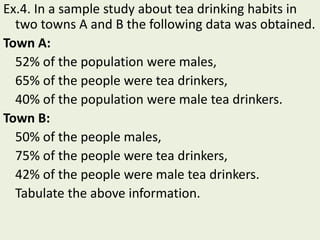
Ex.4. In a sample study about tea drinking habits in
two towns A and B the following data was obtained.
Town A:
52% of the population were males,
65% of the people were tea drinkers,
40% of the population were male tea drinkers.
Town B:
50% of the people males,
75% of the people were tea drinkers,
42% of the people were male tea drinkers.
Tabulate the above information.

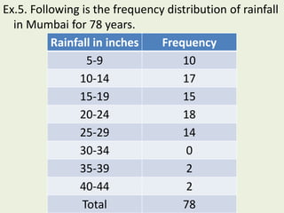
Ex.5. Following is the frequency distribution of rainfall
in Mumbai for 78 years.
Rainfall in inches Frequency
5-9 10
10-14 17
15-19 15
20-24 18
25-29 14
30-34 0
35-39 2
40-44 2
Total 78

1. Obtain class boundaries of 3rd class
2. Find class mark of 1st class
3. Find class width of any class
4. Number of years having less than 25 inches
rainfall
5. Number of years having more than 29 inches
rainfall.

Ex.6.From the following distribution of age of Life
Insurance Policy holders prepare a frequency
distribution and also cumulative frequency
distribution on more than basis.
Age (Yrs.) No. of Policy Holders
Less than 15 9
Less than 25 25
Less than 35 63
Less than 45 86
Less than 55 100

Graphical Representation of Data

• Histogram
• Frequency Polygon
• Multiple Bar Diagram
• Subdivided Bar Diagram

Unit 001Stats (1).pdf

Recommended

Recommended

More Related Content

Similar to Unit 001Stats (1).pdf

Similar to Unit 001Stats (1).pdf (20)

Recently uploaded

Recently uploaded (20)

Unit 001Stats (1).pdf