Travel route scheduling based on user’s preferences using simulated annealing

International Journal of Electrical and Computer Engineering (IJECE)
Vol. 9, No. 2, April 2019, pp. 1275∼1287
ISSN: 2088-8708, DOI: 10.11591/ijpeds.v9i2.pp1275-1287 Ì 1275
Travel route scheduling based on user’s preferences using
simulated annealing
Z.K.A. Baizal, Kemas M. Lhaksmana, Aniq A. Rahmawati, Mizanul Kirom, Zidni Mubarok
Department of Computational Science, Telkom School of Engineering, Telkom Univeristy, Indonesia
Article Info
Article history:
Received Apr 13, 2018
Revised Sep 12, 2018
Accepted Oct 8, 2018
Keywords:
multi-agent system
intelligent travelling planner
travel route scheduling
simulated annealing
traveling salesman problem
ABSTRACT
Nowadays, traveling has become a routine activity for many people, so that many
researchers have developed studies in the tourism domain, especially for the determi-
nation of tourist routes. Based on prior work, the problem of determining travel route
is analogous to finding the solution for travelling salesman problem (TSP). However,
the majority of works only dealt with generating the travel route within one day and
also did not take into account several user’s preference criteria. This paper proposes
a model for generating a travel route schedule within a few days, and considers some
user needs criteria, so that the determination of a travel route can be considered as a
multi-criteria issue. The travel route is generated based on several constraints, such
as travel time limits per day, opening/closing hours and the average length of visit for
each tourist destination. We use simulated annealing method to generate the optimum
travel route. Based on evaluation result, the optimality of the travel route generated by
the system is not significantly different with ant colony result. However, our model is
far more superior in running time compared to Ant Colony method.
Copyright c 2019 Institute of Advanced Engineering and Science.
All rights reserved.
Corresponding Author:
Name Z.K.A. Baizal,
Affiliation Department of Computational Science, Telkom School of Engineering, Telkom University,
Address Jl Telekomunikasi No.1, Jl Terusan Buah Batu, Bojongsoang, Bandung.
Phone 022 7564108
Email baizal@telkomuniversity.ac.id
1. INTRODUCTION
These days, travelling has become a daily need for people, especially during holidays. On most cases,
tourist will try to visit new tourism places they never visit before [1]. Therefore, plenty of tourists want to visit
that places for several days. So, the tourists need to plan their travel. Usually, tourists have travel agent to plan
the travel schedule and guide their trip.
There are many studies that develop the systems that are able to replace travel agent, specifically on
deciding which destination suits the user’s need, as well as determining travel route. This system evolved as
a recommender system, capable of recommending tourism destination and travel routes. The travel routes are
generated based on its opening hours and visiting duration [2]. However, the model in the determination of
the travel route can only accommodate one-day visit time. Vansteenwegen et al utilize Greedy Randomized
Adaptive Search Procedure (GARSP) to develop City Trop Planner for planning route 5 cities in Belgium [3].
Form that research, the model created is able to schedule a travel route for several days with constraints such
as open hours on and rest periods i.e. lunch. However, the selection of that route scheduling is only based
on travel time, whereas in the real world, tourists choose tourism destinations based on many criteria, such as
popularity, the reviews on those destinations, entry fee and so forth.
In many works, the problem of determining travel route is similar to finding the solution from the
Traveling Salesman Problem (TSP) . TSP is a problem where a salesman must visit each node exactly once
with optimal time where the start node and the end node are the same node. In a travel route, TSP can be
Journal Homepage: http://iaescore.com/journals/index.php/IJECE

1276 Ì ISSN: 2088-8708
analogous to visiting tourist attractions exactly once in one day where the start and end node is the tourist’s
lodge. There are plenty of algorithms which can be implemented to solve TSP, i.e.,Genetic Algorithm (GA) [4],
Simulated Annealing (SA) [5], Taboo Search [6], Particle Swarm Optimization [7], Harmony Search [8], Quan-
tum Annealing [9], Ant Colony optimalization (ACO) [10], neural network [11] and so on. We use Simulated
Annealing algorithm (SA) to generate travel route schedule, because SA is an algorithm with the best travel
solution quality based on 3 aspects: mean value, standard deviation, running time [12].
Simulated Annealing is a method to find the solution of combinatorial problem [13, 14], developed
from Metropolish algorithm, which is an algorithm for solving problems in the field of physics. The Metropol-
ish algorithm was developed around 1940’s, utilizing the Monte Carlo simulation process [15]. Simulated
Annealing works by taking behavioral analogy in physics process, particularly the process of freezing or an-
nealing. This process starts when the temperature of the liquid object is still high and then the temperature is
slowly lowered to a specified temperature. If the temperature is done drastically, it will end bad.
The majority of the previous researches developed a model of determining of travel routes in one
day and did not accommodate tourist’s preferences of the desired routes, which probably involve multiple
criteria. This paper proposes a model by adopting Simulated Annealing method, to generate a travel route
schedule within several days, taking into account the three criteria of tourist’s needs: 1). Tourists want to visit
as many attractions as possible within a few days, 2) tourists want to visit the popular destinations, 3) tourists
want a travel route that minimizes the budget. Thus, the problem of determining the travel route is seen as
a multi-criteria problem. To solve the multi-criteria problem, we utilize the concept of multi attribute utility
theory (MAUT). MAUT is a method which is frequently used for evaluating products based on the value of
weight and utilities of some criteria/attributes [16] The weight of each criterion is obtained based on degree
of interest (DOI) of users. DOI is a user degree of interest for each criterion, with the interval [0,1]. Travel
route schedule determination also considers some constraints, which are: 1) travel time limits per day, 2)
opening/closing hours, and 3) the average amount of visit time for each destination. This research is one part of
our research project, to develop a conversation-based recommender system in the tourism domain. The system
will recommend tourist destinations as well as recommend a tour route based on explicitly stated user needs.
This research is one part of our research project, to develop a conversation-based recommender system in the
tourism domain. The system will recommend tourist destinations as well as recommend a tour route based on
explicitly stated user needs. The system generates conversation by utilizing the concept of semantic reasoning
[17, 18, 19]
2. THE SYSTEM OVERVIEW
The system is able to recommend travel route schedule based on user preferences. The proposed
model generates the travel route schedule which is based on Simulated Annealing algorithm. 1 shows the
system overview.
Generally, the steps in generating travel route schedule are as follow:
1. User provides :
(a) Travel Destinations
User is given the opportunity to choose the desired travel destination.
(b) Hotel
The hotel or the lodge where the user stays.
(c) DOI (degree of Interest)
DOI is the user degree of interest to each criterion, as a form of user preferences. The system
accommodates 3 different criteria of needs, which are: 1) tourist want to visit as many places
as possible within a few days (routes are based on travel time), 2) tourist want to visit popular
destinations (routes based on rating), 3) tourists want a travel route that minimized the budget
(routes based on tariff). The value of DOI is between the interval of [0,1].
2. System performs optimal route search with Simulated Annealing algorithm. At this stage, system re-
trieves the destination data and time matrix data from database, for the calculation of fitness value.
3. Once the optimal route is obtained, then the system performs the scheduling process using the accumu-
lated travel time and the duration of visits on each tourist destination.
Int J Elec & Comp Eng Vol. 9, No. 2, April 2019 : 1275 – 1287

Int J Elec & Comp Eng ISSN: 2088-8708 Ì 1277
Figure 1. The Overview of the System
4. The system displays the travel route schedule (maximum in 3 days as well the visual display of the route,
by utilizing the help of google maps API).
3. SIMULATED ANNEALING FOR ROUTE SCHEDULING
Basically, the determination of travel route can be viewed as a problem to ﬁnd the solution for TSP.
Generally, the optimal TSP route is determined based on the time or nearest distance. This research proposes
a model to generate travel route schedule (TSP) based on 3 criteria (multi criteria). As discussed in section
2, these three criteria can be considered as parameters for route determination, which are: 1). Travel time, 2).
Rating, 3). The price of each tourist destination. The time travel is taken from Google Maps, taking the typical
time instead of real time, since tourists can plan the tours in advance. In addition, there is also checking for
constraints such as opening and closing hours on each accumulation of each tourist destination schedule and
the maximum time of tourist visits in one day.
The steps of determining travel route are as follow:
3.1. Parameter Initialization
Some of the initialized Simulated Annealing parameters are: initial temperature, cooling rate, stopping
temperature. The parameters are used to determine the number of iteration in the annealing process. At the
stage of parameter initialization, the parameters used are taken by experiment.
(a) The Initialization of The First (tour) Solution
In this stage, the system will generate initial (tour) solution. The initial generation of tour can be done
by making tour randomly.
(b) The Formation of New Tour (Solution)
The formation of new tour (solution) as the candidate for the solution. This new solution can be a
better solution than the previous solution. For the formation of a new (tour) solution, the system uses the
swapping mutation method. Swapping mutation is done by selecting 2 nodes randomly from the previous
solution. After that, the nodes are reversed to generate a new (tour) solution. Here’s an illustration of
generating a new tour (solution).
• Solution before
1 2 4 5 3
Travel route scheduling based on... (Z.K.A. Baizal, Kemas M. Lhaksmana)

1278 Ì ISSN: 2088-8708
Figure 2. The steps of generating travel route schedule
• New solution
1 2 5 4 3
(c) The Determination of Time Accumulation
After two (tour) solutions obtained, its total time will be accumulated to obtain the tourist route per day.
Each tour visit begins and ends at the hotel selected by user. Every day, the tour begins at 08.00 until
20.00. To determine the travel route per day, the system checks the schedule of the opening and closing
hours each destination. The algorithm for time accumulation is explained in Algorithm 1.
Algorithm 1 AcumulateTime (solution) input: solution, output: perDaySolution
1: perDaySolution ← [];
2: currentnode ← hotel;
3: for i in range(solution) do
4: arrivalTime(node[i])=finishedTime(currentnode) + travel(currentnode,node[i])
5: finishedTime(node[i])=arrivalTime(node[i]) + duration(node[i])
6: if arrivalTime(node[i]) in Time Constraints then
7: if arrivalTime(node[i]) in constraint open and closed time then
8: put node[i] into perDaySolution list;
9: currentnode ← node[i]
10: end if
11: end if
12: end for
13: return perDaySolution;
The steps in algorithm 1 can be explained as follows,
• If the known (tour) solution is as follow,
1 2 4 5 3 7 6 8
With the open and close hours are shown in Table 1.
• Time Calculation
The time displayed in the scheduling is the time range from arrival time until finish of each tourist

Table 1. The opening and closing hours of each destination
Node Opening and closing hours
1 00.00 - 00.00
2 07.00 - 22.00
4 08.00 - 12.00
5 08.00 - 20.00
3 08.00 - 20.00
7 08.00 - 20.00
6 08.00 - 20.00
8 08.00 - 20.00
Table 2. The result of time accumulation of each destination
1 08.00 - 10.00
2 11.00 - 12.00
4 14.00 - 17.00
destination
AT(node[i]) =
FT(hotel) + T(hotel, node[i]) if i = 0
FT(node[i − 1]) + T(node[i − 1], node[i]) otherwise
(1)
where,
AT(node[i])= the arrival time on ith destination.
FT(node[i])= the finished time on ith destination.
T(a, b)= time travel between two tourist destination from point A to point B. Illustrated as follows:
Table 2 shows the time accumulation of each tourist destination in the range solution. Range so-
lution is the number of tourist destination, then at each accumulated destination, the system checks
the opening and closing hours according to Table 1. Because the 4th
node exceeds the closing
time, then
1 2 4 5 3 7 6 8
The node will be saved for the next day route, then the scheduling continues to the next node
until the time constraint is met. Time constraint has the value of ”true” when the time range is
between 08.00-20.00 (in accordance with the time limit of tourist visits in 1 day). Based on the
accumulation of time, the results of the tour in one day can be seen in Table 3.
• Fitness Value Calculation
The fitness value in Simulated Annealing, commonly referred to energy [20]. The calculation of
fitness value aims for the selection of the (tour) solution, so that the best solution can be determined.
In this research, optimized tour search is done by two kinds of fitness value calculation:
a Based on single criteria (travel time). The calculation of fitness value only uses a single crite-
rion, which is travel time. The fitness value calculation can be formulated with the following
equation:
Time(x) =
duration(hotel, x0) +
n−1
i=1 duration(xi,xi+1)
n−1 + duration(xj, hotel)
3
(2)
Table 3. The tour result per day
1 08.00 - 10.00
2 11.00 - 12.00
5 13.00 - 15.00
3 15.30 - 16.00
7 18.00 - 19.30

1280 Ì ISSN: 2088-8708
where,
X= The travel tour solution of x1, x2, ..., xn.
Time(X)= Fitness value based on travel time
n = Length of node or tour
xi = The ith node/tourist spot
Duration(a, b)= Trip duration from node a to b
b Based on multi criteria (time, rating, and fare)
The fitness value calculated by using Multi Attribute Utility Theory (MAUT) method, includ-
ing travel time, rating and fare of each tourist destination. The fitness value can be formulated
as follows,
F(time(X), rating(X), tariff(X)) =
w1 × time(X) + w2 × rating(X) + w3 × tariff(X)
3
(3)
where,
w1 = weight of travel time
w2 = weight of rating
w3 = weight of fare
The definitions for time(X) is provided in Eq. 2, while rating(X) and tariff(X) are pro-
vided in Eq. 5 and 6, respectively. In this case, normalization is required in determining
duration(a, b) as defined in Eq. 4
duration(a, b) =
duration(a, b) +
n−1
i=1 duration(xi,xi+1)
n−1 + duration(xj, hotel)
3
(4)
where n minduration is the minimum value duration and maxduration refers to the maximum
value of duration. The fitness value which is formulated based on the popularity rating is
formulated as follows,
rating(a, b) =
n
i=1 rating(xi)
n
(5)
Where n is the length of the solution. As for the fitness value which is based on tariff, the
formulation is as follows,
tariff(a, b) =
n
i=1 tariff(xi)
n
(6)
where n is the length of the solution. Normalization operations for rating(X) and tariff(X)
are performed as the same as that of duration(a, b).
• Acceptance Probability Calculation
After the fitness value from the new (tour) solution is obtained, we have to checks whether the new
(tour) solution is a better (tour) than previous solution by this acceptance probability. The algorithm
to determine the best solution candidate is shown in Algorithm 2 [21].
Algorithm 2 Acceptence Probability (solution,newSolution)
input: solution and newSolution output: solution
1: if newSolution > solution then
2: solution ← newSolusion;
3: if random(0, 1) < probability(solution, newSolution) then
4: solution ← newSolusion;
5: end if
6: end ifreturn solution;
The function of acceptance probability can be formulated as follows [22]
Paccept(S(i), S(i − 1))
1 if S(i) > S(i − 1)
exp−∆S
T otherwise
(7)

where,
Paccept = The acceptance probability function to obtain the best solution candidate
T = Temperature.
S(i) = Solution gained on iteration-i
∆S = F(S(i − 1)) − F(S(i))
• Temperature decrease item
The each iteration is done to decrease the temperature value. The common way to decrease this
temperature is the geometric cooling schedule [21]. Formally, the temperature drop can be formu-
lated as follows,
T = coolingrate ∗ T (8)
where T is temperature and coolingrate is a constant for the decrease in the Simulated Annealing
algorithm
The iteration is complete if the temperature value is less than the stopping temperature. Based on
this iteration, we get a solution (tour) that will be taken as a tourist route in one day.
4. EVALUATION
For evaluation, we have to determine the best parameters of the simulated annealing algorithm, such
as temperature T, cooling rate α, and stopping temperature. We conduct some tests for it, by combining those
parameters. For each combination, a trial was done 10 times to get the test results.
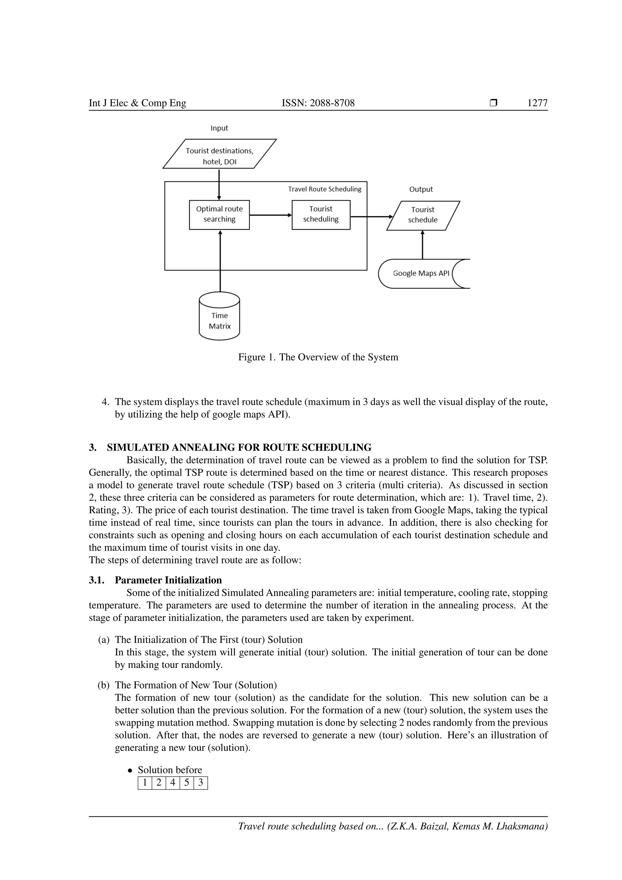
Table 4 shows the result of the parameter test with predetermined interval value. The best parameter
combination is determined from the total node, running time, and total days. Based on table 4, we notice that
the best combination is temperature = 15000, cooling rate = 0.99, and stopping temperature = 0.0002. After
obtaining the best parameters, then those parameters will be used on system performance testing.
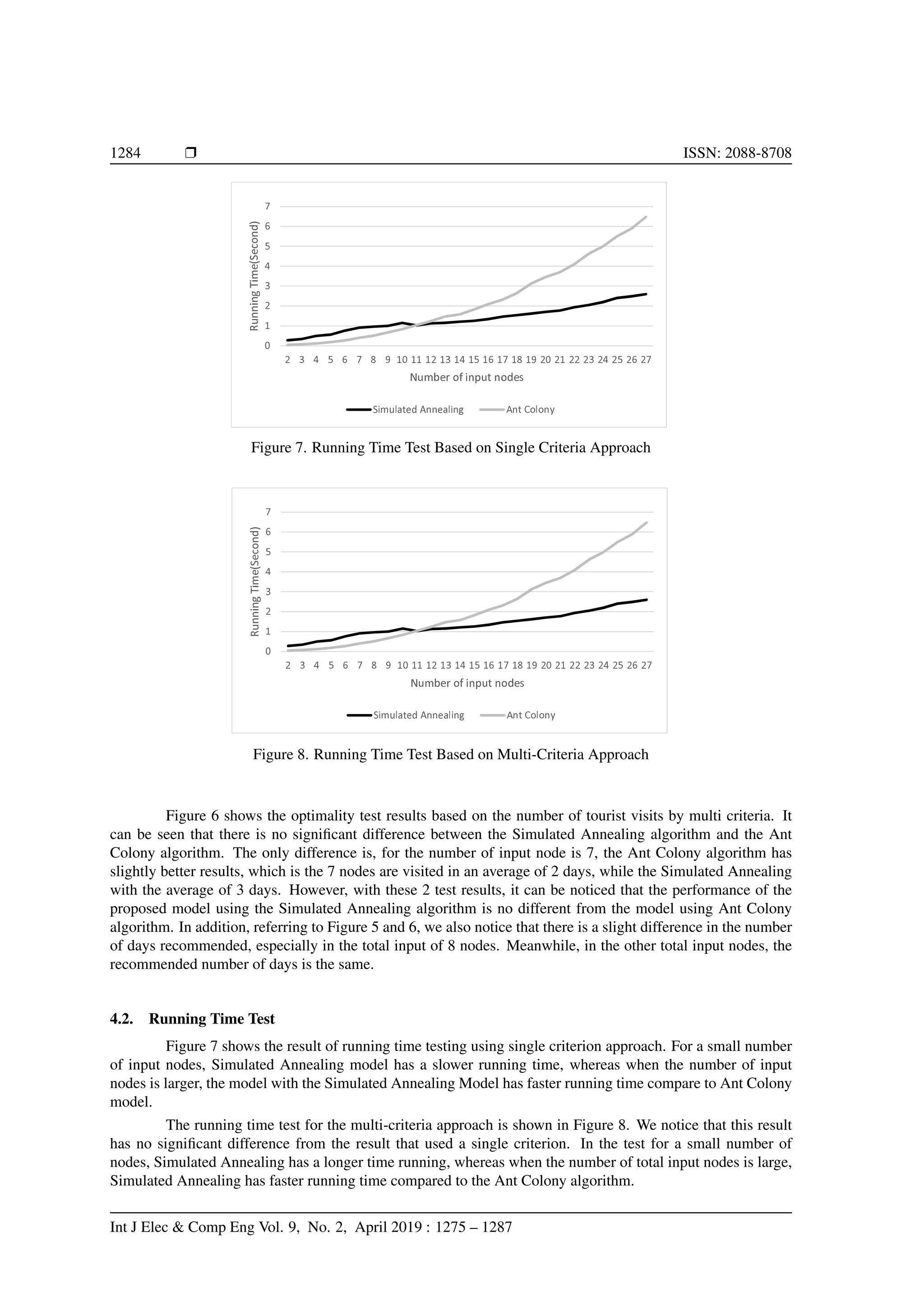
We evaluate the system by considering two aspects; performance test and running time test. The
results of the proposed model will be compared with the results of the ant colony optimization algorithm, in
our previous work [23]. The performance test use single criterion (time) and multi criteria (time, rating, fare).
We involve 28 tourist destination. This test is done in 10 trials. The performance is determined by the optimum
aspect of the travel route resulted and also the running time.
4.1. Travel Tour Optimality Test
4.1.1. The Optimality Based on Number of Tourist Places (Nodes) in Tour
Figure 3 shows the test results based on the number of nodes (tourist destinations) in a tour using a
single criterion (travel time) approach. For the input nodes 2 to 7 nodes, we notice that there are no difference
performance for both algorithm. Meanwhile, input nodes 8 through 21 using the Ant Colony algorithm, produce
more nodes in the tour, compared to Simulated Annealing algorithm. But for many input nodes (22 to 27), the
number of nodes in tour for the Simulated Annealing algorithm has better results than the Ant Colony algorithm.
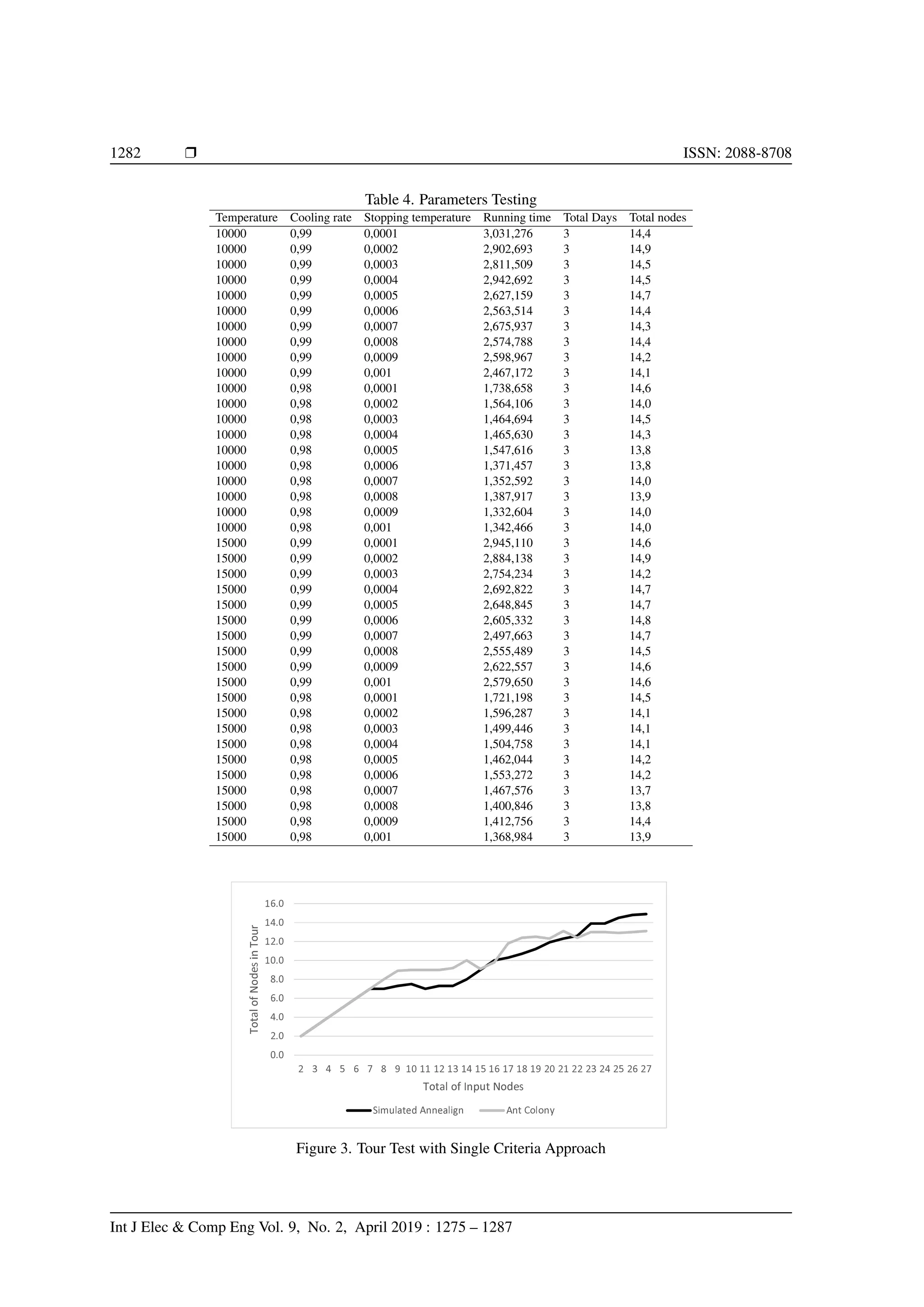
Figure 4 shows the test results based on the number of nodes in best tour using multi criteria approach.
It can be seen that these results do not have a significant difference with the results obtained from the single
criterion approach. The Ant Colony algorithm has better results when the input nodes are 8 to 21, while the
Simulated Annealing algorithm has better results with input nodes of 22 to 27. Based on both test results, we
notice that: 1) the number of nodes in tour, no significant trend differences between single criterion and multi
criteria approach, 2) For a small number of input nodes, Ant Colony is superior, however for the larger number
of input nodes (in this case is over 22 nodes), the model proposed using Simulated Annealing is better in terms
of optimality.
4.1.2. The Optimality Based on the Amount of Visit Days
Optimality test based on the amount of days of tourist visit by using single criteria approach, is shown
by Figure 5. It shows that the result of Simulated Annealing algorithm has no significant difference to the
Ant Colony algorithm. The difference occurs only in the number of input nodes of 7, where the Simulated
Annealing algorithm has slightly better results.

1282 Ì ISSN: 2088-8708
Table 4. Parameters Testing
Temperature Cooling rate Stopping temperature Running time Total Days Total nodes
10000 0,99 0,0001 3,031,276 3 14,4
10000 0,99 0,0002 2,902,693 3 14,9
10000 0,99 0,0003 2,811,509 3 14,5
10000 0,99 0,0004 2,942,692 3 14,5
10000 0,99 0,0005 2,627,159 3 14,7
10000 0,99 0,0006 2,563,514 3 14,4
10000 0,99 0,0007 2,675,937 3 14,3
10000 0,99 0,0008 2,574,788 3 14,4
10000 0,99 0,0009 2,598,967 3 14,2
10000 0,99 0,001 2,467,172 3 14,1
10000 0,98 0,0001 1,738,658 3 14,6
10000 0,98 0,0002 1,564,106 3 14,0
10000 0,98 0,0003 1,464,694 3 14,5
10000 0,98 0,0004 1,465,630 3 14,3
10000 0,98 0,0005 1,547,616 3 13,8
10000 0,98 0,0006 1,371,457 3 13,8
10000 0,98 0,0007 1,352,592 3 14,0
10000 0,98 0,0008 1,387,917 3 13,9
10000 0,98 0,0009 1,332,604 3 14,0
10000 0,98 0,001 1,342,466 3 14,0
15000 0,99 0,0001 2,945,110 3 14,6
15000 0,99 0,0002 2,884,138 3 14,9
15000 0,99 0,0003 2,754,234 3 14,2
15000 0,99 0,0004 2,692,822 3 14,7
15000 0,99 0,0005 2,648,845 3 14,7
15000 0,99 0,0006 2,605,332 3 14,8
15000 0,99 0,0007 2,497,663 3 14,7
15000 0,99 0,0008 2,555,489 3 14,5
15000 0,99 0,0009 2,622,557 3 14,6
15000 0,99 0,001 2,579,650 3 14,6
15000 0,98 0,0001 1,721,198 3 14,5
15000 0,98 0,0002 1,596,287 3 14,1
15000 0,98 0,0003 1,499,446 3 14,1
15000 0,98 0,0004 1,504,758 3 14,1
15000 0,98 0,0005 1,462,044 3 14,2
15000 0,98 0,0006 1,553,272 3 14,2
15000 0,98 0,0007 1,467,576 3 13,7
15000 0,98 0,0008 1,400,846 3 13,8
15000 0,98 0,0009 1,412,756 3 14,4
15000 0,98 0,001 1,368,984 3 13,9
Ϭ͘Ϭ
Ϯ͘Ϭ
ϰ͘Ϭ
ϲ͘Ϭ
ϴ͘Ϭ
ϭϬ͘Ϭ
ϭϮ͘Ϭ
ϭϰ͘Ϭ
ϭϲ͘Ϭ
Ϯ ϯ ϰ ϱ ϲ ϳ ϴ ϵ ϭϬ ϭϭ ϭϮ ϭϯ ϭϰ ϭϱ ϭϲ ϭϳ ϭϴ ϭϵ ϮϬ Ϯϭ ϮϮ Ϯϯ Ϯϰ Ϯϱ Ϯϲ Ϯϳ
dŽ
ƚĂůŽ
Ĩ
E
Ž
Ě
Ğ
Ɛ
ŝŶ
dŽ
Ƶ
ƌ
dŽƚĂů ŽĨ /ŶƉƵƚ EŽĚĞƐ
^ŝŵƵůĂƚĞĚ ŶŶĞĂůŝŐŶ Ŷƚ ŽůŽŶǇ
Figure 3. Tour Test with Single Criteria Approach
Int J Elec Comp Eng Vol. 9, No. 2, April 2019 : 1275 – 1287

Int J Elec Comp Eng ISSN: 2088-8708 Ì 1283
Ϭ͘Ϭ
Ϯ͘Ϭ
ϰ͘Ϭ
ϲ͘Ϭ
ϴ͘Ϭ
ϭϬ͘Ϭ
ϭϮ͘Ϭ
ϭϰ͘Ϭ
ϭϲ͘Ϭ
dŽ
ƚĂůŽ
Ĩ
E
Ž
Ě
Ğ
Ɛ
ŝŶ
dŽ
Ƶ
ƌ
dŽƚĂů ŽĨ /ŶƉƵƚ EŽĚĞƐ
^ŝŵƵůĂƚĞĚ ŶŶĞĂůŝŶŐ Ŷƚ ŽůŽŶǇ
Figure 4. Tour Test with Multi Criteria Approach
Ϭ
Ϭ͘ϱ
ϭ
ϭ͘ϱ
Ϯ
Ϯ͘ϱ
ϯ
ϯ͘ϱ
E
Ƶŵ
ďĞƌŽĨĚĂǇƐŽĨǀŝƐŝƚ
EƵŵďĞƌ ŽĨ ŝŶƉƵƚ ŶŽĚĞƐ
Figure 5. Number of Days Test with Single Criteria Approach
Ϭ
Ϭ͘ϱ
ϭ
ϭ͘ϱ
Ϯ
Ϯ͘ϱ
ϯ
ϯ͘ϱ
EƵŵ
ďĞƌŽĨĚĂǇƐ
Figure 6. Number of Days with Multi Criteria Approach

1284 Ì ISSN: 2088-8708
Ϭ
ϭ
Ϯ
ϯ
ϰ
ϱ
ϲ
ϳ
ZƵŶŶŝŶŐ
dŝŵ
Ğ;^ĞĐŽŶĚͿ
Figure 7. Running Time Test Based on Single Criteria Approach
Ϭ
ϭ
Ϯ
ϯ
ϰ
ϱ
ϲ
ϳ
ZƵŶŶŝŶŐ
dŝŵ
Ğ;^ĞĐŽŶĚͿ
Figure 8. Running Time Test Based on Multi-Criteria Approach
Figure 6 shows the optimality test results based on the number of tourist visits by multi criteria. It
can be seen that there is no signiﬁcant difference between the Simulated Annealing algorithm and the Ant
Colony algorithm. The only difference is, for the number of input node is 7, the Ant Colony algorithm has
slightly better results, which is the 7 nodes are visited in an average of 2 days, while the Simulated Annealing
with the average of 3 days. However, with these 2 test results, it can be noticed that the performance of the
proposed model using the Simulated Annealing algorithm is no different from the model using Ant Colony
algorithm. In addition, referring to Figure 5 and 6, we also notice that there is a slight difference in the number
of days recommended, especially in the total input of 8 nodes. Meanwhile, in the other total input nodes, the
recommended number of days is the same.
4.2. Running Time Test
Figure 7 shows the result of running time testing using single criterion approach. For a small number
of input nodes, Simulated Annealing model has a slower running time, whereas when the number of input
nodes is larger, the model with the Simulated Annealing Model has faster running time compare to Ant Colony
model.
The running time test for the multi-criteria approach is shown in Figure 8. We notice that this result
has no signiﬁcant difference from the result that used a single criterion. In the test for a small number of
nodes, Simulated Annealing has a longer time running, whereas when the number of total input nodes is large,
Simulated Annealing has faster running time compared to the Ant Colony algorithm.

5. CONCLUSION
Based on the result of performance test, it can be concluded that there is no significant difference
performance (i.e. optimality and running time), between travel tour with single criterion and multi-criteria
approach. Thus, determining the travel route based on multi-criteria user preferences that covers: 1) Tourists
want to visit as many tourist attractions as possible within several days, 2) Tourists want to visit the popular
tourist destinations, and 3) Tourists want a travel route that can minimize the budget, can be implemented
without interfering on the performance.
From the optimality aspect, it can be concluded that Simulated Annealing is able to schedule a travel
route with good results. For the input nodes that has the same number as the number of tours, it will relatively
have similar results, this is due to the limit of the number of days so that the number of tourist destinations
visited have a relatively equal number. Likewise, on the length of running time with the high number of input
nodes, it does not have a significant difference due to the number of nodes obtained relatively the same, so that
the fitness value calculation that affects the running time has the same relative results.
From the comparison of test results to Ant Colony algorithm, the result of the number of tours in the
route using Simulated Annealing has a better result for the case on the large amount of data input. This is
because the combination of candidate solutions produced has a wide range of variety. After that, if it is viewed
from the running time of Simulated Annealing on the case of scheduling the travel route, on the average it has
faster running time than the Ant Colony algorithm.
6. ACKNOWLEDGMENTS
We would like to thank the ministry of Research, Technology and Higher Education of the Republic
of Indonesia that has supported us in conducting this research, in the institution national strategic research
scheme.
REFERENCES
[1] A. Moreno, A. Valls, D. Isern, L. Marin, and J. Borràs, “Sigtur/e-destination: ontology-based personalized
recommendation of tourism and leisure activities,” Engineering Applications of Artificial Intelligence,
vol. 26, no. 1, pp. 633–651, 2013.
[2] L. Sebastia, I. Garcia, E. Onaindia, and C. Guzman, “e-tourism: a tourist recommendation and planning
application,” International Journal on Artificial Intelligence Tools, vol. 18, no. 05, pp. 717–738, 2009.
[3] P. Vansteenwegen, W. Souffriau, G. V. Berghe, and D. Van Oudheusden, “The city trip planner: an expert
system for tourists,” Expert Systems with Applications, vol. 38, no. 6, pp. 6540–6546, 2011.
[4] B. Kaur and U. Mittal, “Optimization of tsp using genetic algorithm,” Advances in Computational Sci-
ences and Technology, vol. 3, no. 2, pp. 119–125, 2010.
[5] D. J. Ram, T. Sreenivas, and K. G. Subramaniam, “Parallel simulated annealing algorithms,” Journal of
parallel and distributed computing, vol. 37, no. 2, pp. 207–212, 1996.
[6] A. Miseviˇcius, “Using iterated tabu search for the traveling salesman problem,” Information technology
and control, vol. 32, no. 3, 2004.
[7] J. Kennedy, “Particle swarm optimization,” in Encyclopedia of machine learning. Springer, 2011, pp.
760–766.
[8] Z. W. Geem, J. H. Kim, and G. Loganathan, “A new heuristic optimization algorithm: harmony search,”
simulation, vol. 76, no. 2, pp. 60–68, 2001.
[9] A. Finnila, M. Gomez, C. Sebenik, C. Stenson, and J. Doll, “Quantum annealing: a new method for
minimizing multidimensional functions,” Chemical physics letters, vol. 219, no. 5-6, pp. 343–348, 1994.
[10] C.-S. Lee, Y.-C. Chang, and M.-H. Wang, “Ontological recommendation multi-agent for tainan city
travel,” Expert Systems with Applications, vol. 36, no. 3, pp. 6740–6753, 2009.
[11] W. O. Vihikan, D. Putra, I. K. Gede, and I. Dharmaadi, “Foreign tourist arrivals forecasting using recurrent
neural network backpropagation through time.” Telkomnika, vol. 15, no. 3, 2017.
[12] M. Antosiewicz, G. Koloch, and B. Kamiński, “Choice of best possible metaheuristic algorithm for the
travelling salesman problem with limited computational time: quality, uncertainty and speed,” Journal of
Theoretical and Applied Computer Science, vol. 7, no. 1, pp. 46–55, 2013.
[13] S. Kirkpatrick, C. D. Gelatt, M. P. Vecchi et al., “Optimization by simulated annealing,” science, vol. 220,
no. 4598, pp. 671–680, 1983.

1286 Ì ISSN: 2088-8708
[14] V. ˇCerný, “Thermodynamical approach to the traveling salesman problem: An efficient simulation algo-
rithm,” Journal of optimization theory and applications, vol. 45, no. 1, pp. 41–51, 1985.
[15] N. Metropolis, A. W. Rosenbluth, M. N. Rosenbluth, A. H. Teller, and E. Teller, “Equation of state
calculations by fast computing machines,” The journal of chemical physics, vol. 21, no. 6, pp. 1087–
1092, 1953.
[16] R. Schäfer, “Rules for using multi-attribute utility theory for estimating a user’s interests,” in Ninth Work-
shop Adaptivität und Benutzermodellierung in Interaktiven Softwaresystemen, 2001, pp. 8–10.
[17] Z. A. Baizal, D. H. Widyantoro, and N. U. Maulidevi, “Factors influencing user’s adoption of conversa-
tional recommender system based on product functional requirements,” TELKOMNIKA (Telecommunica-
tion Computing Electronics and Control), vol. 14, no. 4, pp. 1575–1585, 2016.
[18] ——, “Query refinement in recommender system based on product functional requirements,” in Advanced
Computer Science and Information Systems (ICACSIS), 2016 International Conference on. IEEE, 2016,
pp. 309–314.
[19] Z. A. Baizal, Y. R. Murti et al., “Evaluating functional requirements-based compound critiquing on con-
versational recommender system,” in Information and Communication Technology (ICoIC7), 2017 5th
International Conference on. IEEE, 2017, pp. 1–6.
[20] D. S. Johnson, C. R. Aragon, L. A. McGeoch, and C. Schevon, “Optimization by simulated annealing:
an experimental evaluation; part i, graph partitioning,” Operations research, vol. 37, no. 6, pp. 865–892,
1989.
[21] S.-h. Zhan, J. Lin, Z.-j. Zhang, and Y.-w. Zhong, “List-based simulated annealing algorithm for traveling
salesman problem,” Computational intelligence and neuroscience, vol. 2016, p. 8, 2016.
[22] D. Henderson, S. H. Jacobson, and A. W. Johnson, “The theory and practice of simulated annealing,” in
Handbook of metaheuristics. Springer, 2003, pp. 287–319.
[23] Z. A. Baizal, A. A. Rahmawati, K. M. Lhaksmana, M. Z. Mubarok, and M. Qadrian, “Generating travel
itinerary using ant collony optimization,” TELKOMNIKA (Telecommunication Computing Electronics and
Control), vol. 16, no. 3, 2018.
BIOGRAPHIES OF AUTHORS
Z.K.A. Baizal received the BS degree from the Gadjah Mada University, Yogyakarta, Indonesia,
in 1998. He joined Faculty of Informatics at Telkom University in 1999. He received the MS
degrees from computer science from Gadjah Mada University in 2003. In 2017, he is received
PhD degree in electrical engineering informatics at Institut Teknologi Bandung (ITB), Indonesia.
His research interests include artificial intelligence, information extraction, ontology, as well as
information classification.
In International Journal of Human-Computer System (Elsevier), Journal of ICT Research and Ap-
plications, and other scientific publications, he has served as invited reviewer.
Kemas M. Lhaksmana received the Ph.D. degree in informatics from Kyoto University, Kyoto,
Japan, in 2016, and the master?s degree in information systems development from HAN University
of Applied Sciences, Arnhem, The Netherlands, in 2009. He has been a Lecturer with the Faculty
of Informatics, Telkom University, Bandung, Indonesia, since 2011. His current research interests
include multiagent systems, services computing, and Internet of Things.

Aniq Rohmawati completed M.Si in 2012 at Institut Teknologi Bandung (ITB). Aniq Rohmawati
has been staff member at Telkom University since 2015. She did bachelor degree at Airlangga Uni-
versity during 2006-2010. On March 5-18 2018, she granted research school ’Recent developments
in stochastic dynamic and stochastic analysis’, funded by The Centre International de Mathtiques
Pures et Appliqu (CIMPA). Research interest: applied probability, computational statistics, time
series forecasting, and quantitative risk.
Mizanul Kirom got a Bachelor degree on Informatics Engineering, Telkom university in 2017.
He works as a research team member to develop a recommender system of tourism applications
in 2016-2017. Now, he joined at Braincode Solution as a scala developer. He is interested in big
data, artiﬁcial intelligence and software development. He have did some project about geographic
information system(GIS) Application.
Zidni Mubarok got a Bachelor degree on computational science, Telkom university in 2017. He
has interest in Artiﬁcial Intelligence. He has work experience for almost 3 years in PT. Bandung
Zona Teknologi, The biggest project he ever undertaken was to create an HPC Insfrastucture for the
National Nuclear Regulatory Agency (BAPETEN) to run cooling simulations on nuclear reactors.

Travel route scheduling based on user’s preferences using simulated annealing

More Related Content

What's hot

Similar to Travel route scheduling based on user’s preferences using simulated annealing

More from IJECEIAES

Recently uploaded

Travel route scheduling based on user’s preferences using simulated annealing