This book provides a comprehensive overview of transformer engineering. It covers topics such as transformer fundamentals, magnetic characteristics, impedance characteristics, eddy currents and winding losses, stray losses in structural components, short-circuit stresses and strength, surge phenomena, insulation design, cooling systems, structural design, special transformers, electromagnetic fields and computations, transformer-system interactions and modeling, and monitoring and diagnostics. The second edition contains three new chapters and has been updated throughout to reflect recent advances in the field. The book provides both theoretical and practical guidance useful for engineers working in the transformer industry.


![Transformer Fundamentals 11
b. Series reactors: These reactors are connected in series with generators, feeders,
and transmission lines to limit fault currents under short-circuit conditions. These
reactors should have linear magnetic characteristics under fault conditions. They
should be designed to withstand the mechanical and thermal effects of short
circuits. The winding of series reactors used for transmission lines is of the fully
insulated type since both the ends should be able to withstand lightning voltages.
The value of the series reactors has to be judiciously chosen because a higher
value reduces the power transfer capability of the lines. Smoothing reactors used
in HVDC transmission systems smoothen out the ripple in the DC voltage.
1.3 Principles and the Equivalent Circuit
1.3.1 Ideal transformer
Transformers work on the principle of electromagnetic induction, according to
which a voltage is induced in a coil linking to a changing flux. Figure 1.2 shows
a single-phase transformer consisting of two windings, wound on a magnetic
core and linked by a mutual flux m
I . The transformer is in no-load condition
with its primary connected to a source of sinusoidal voltage of frequency f Hz.
The primary winding draws a small excitation current, i0 (instantaneous value),
from the source to set up the flux m
I in the core. All the flux is assumed to be
contained in the core (no leakage). Windings 1 and 2 have N1 and N2 turns
respectively. The instantaneous value of the induced electromotive force in
winding 1 due to the mutual flux is
dt
d
N
e m
I
1
1 . (1.1)
Equation 1.1 gives the circuit viewpoint; there is a flux-viewpoint also [1], in
which the induced voltage (counter electromotive force) is represented as
)
/
(
1
1 dt
d
N
e m
I
. An elaborate explanation for both the viewpoints is given in
[2]. If the winding is further assumed to have zero resistance (with its leakage
reactance already neglected), then
1
1 e
v . (1.2)
Since 1
v (instantaneous value of the applied voltage) is sinusoidally varying, the
flux m
I must also be sinusoidal in nature varying with frequency f. Let
t
mp
m Z
I
I sin (1.3)
where mp
I is the peak value of mutual flux m
I and Z = 2 S f rad/sec. After
substituting the value of m
I in Equation 1.1, we obtain
t
N
e mp Z
I
Z cos
1
1 . (1.4)
www.EngineeringBooksPDF.com](https://image.slidesharecdn.com/transformer-engineering-design-technology-and-diagnostics-second-edition-pdf-230506172819-680afe24/85/transformer-engineering-design-technology-and-diagnostics-second-edition-pdf-pdf-32-320.jpg)


![Transformer Fundamentals 23
in kV and the base volt-amperes in MVA. Hence, the base impedances on LV
and HV sides can be calculated as
b
bL
bL
Z
MVA
kV 2
and
b
bH
bH
Z
MVA
V
k 2
. (1.51)
For three-phase transformers, the total three-phase power in MVA and line-to-
line voltage in kV have to be taken as the base values. It can be shown that when
ohmic value of impedance is transferred from one side to the other, the
multiplying factor is the ratio of squares of line-to-line voltages of both sides
irrespective of whether the transformer connection is star-star or star-delta [3].
1.5 Open-Circuit and Short-Circuit Tests
Parameters of the equivalent circuit can be determined by open-circuit (no-load)
and short-circuit (load) tests. The open-circuit test determines the shunt
parameters of the equivalent circuit of Figure 1.5. The circuit diagram for
conducting the test is shown in Figure 1.8 (a). The rated voltage is applied to
one winding and the other winding is kept open. Usually, LV winding is
supplied since a low voltage supply is generally available. The no-load current is
a very small percentage (0.2 to 2%) of the full load current; lower percentage
values are observed for larger transformers (e.g., the no-load current of a 300
MVA transformer can be as small as 0.2%). Also, the leakage impedance value
is much smaller than those of the shunt branch parameters. Therefore, the
voltage drop in the LV resistance and leakage reactance is negligible as
compared to the rated voltage ( 1
1 E
V #
? in Figure 1.5, and 0
T can be taken as
the angle between V1 and I0). The input power measured by the wattmeter
consists of the core loss and the primary winding ohmic-loss. If the no-load
current is 1% of the full load current, the ohmic-loss in the primary winding
resistance is just 0.01% of the load loss at the rated current; the value of the
winding loss is negligible as compared to the core loss. Hence, the entire
wattmeter reading can be taken as the core loss. The equivalent circuit of Figure
1.5 (b) is simplified to that shown in Figure 1.8 (b).
Im
W A
V
V
I
HV
I0
1 V1
0
I
R
LV
c
c
Xm
(a) (b)
Figure 1.8 Open-circuit test.
www.EngineeringBooksPDF.com](https://image.slidesharecdn.com/transformer-engineering-design-technology-and-diagnostics-second-edition-pdf-230506172819-680afe24/85/transformer-engineering-design-technology-and-diagnostics-second-edition-pdf-pdf-44-320.jpg)


![26 Chapter 1
1
eq
R is the equivalent AC resistance referred to the primary (HV) winding,
which accounts for the losses in the DC resistance of the windings, the eddy
losses in the windings and the stray losses in structural parts. It is not practical to
apportion the stray losses to the two windings. Hence, if the resistance parameter
is required to be known for each winding, it is usually assumed that
1
'
2
1 )
2
/
1
( eq
R
R
R . Similarly, it is assumed that '
L
L X
X 2
1 , although it is not
strictly true. Since % R is much smaller than % Z, in practice the percentage
reactance (% X) is taken to be the same as the percentage impedance (% Z). This
approximation, however, may not be true for small distribution transformers.
1.6 Voltage Regulation and Efficiency
Since many electrical devices and appliances operate most effectively at their
rated voltage, it is necessary that the output voltage of a transformer be within
narrow limits when the magnitude and power factor of loads vary. Voltage
regulation is an important performance parameter of transformers as it
determines the quality of electricity supplied to consumers. The voltage
regulation for a specific load is defined as a change in the magnitude of the
secondary voltage after removal of the load (the primary voltage being held
constant) expressed as a fraction of the secondary voltage corresponding to the
no-load condition.
Regulation (p.u.) =
oc
oc
V
V
V
2
2
2
(1.61)
where 2
V is the secondary terminal voltage at a specific load and oc
2
V is the
secondary terminal voltage when the load is removed. For the approximate
equivalent circuit of Figure 1.7 (b), if all the quantities are referred to the
secondary side, the voltage regulation for a lagging power factor load is given as
[4]
Regulation (p.u.) =
oc
eq
eq
V
X
I
R
I
2
2
2
2
2
2
2 sin
cos T
T
2
2
2
2
2
2
2
2 sin
cos
2
1
¸
¸
¹
·
¨
¨
©
§
oc
eq
eq
V
R
I
X
I T
T
(1.62)
where 2
eq
R and 2
eq
X are the equivalent resistance and leakage reactance of the
transformer referred to the secondary side respectively. The secondary load
www.EngineeringBooksPDF.com](https://image.slidesharecdn.com/transformer-engineering-design-technology-and-diagnostics-second-edition-pdf-230506172819-680afe24/85/transformer-engineering-design-technology-and-diagnostics-second-edition-pdf-pdf-47-320.jpg)


![ª º
37
2
Magnetic Characteristics
The magnetic circuit is an important active part of transformers, which transfers
electrical energy from one circuit to another. It is in the form of a laminated iron
core structure which provides a low reluctance path to the magnetic flux
produced by an excited winding. Most of the flux is contained in the core, which
reduces stray losses in structural parts. Due to research and development efforts
[1] by steel and transformer manufacturers, materials with improved
characteristics have been developed and employed with better core building
technologies. In the early days of transformer manufacturing, inferior grades of
laminated steel (according to today’s standards) were used with associated high
losses and magnetizing volt-amperes. Later, it was found that an addition of
silicon (4 - 5%) improved the performance characteristics of the material
significantly, due to a marked reduction in its eddy loss on account of an
increase in resistivity and permeability. Its hysteresis loss also reduced due to a
decrease in the area of the B-H loop. Since then the silicon steels have been in
use as the core material in most transformers.
The addition of silicon also helps to reduce aging effects. Although silicon
makes the material brittle, the deterioration in the property is not to an extent
that can pose problems during the core building process. Subsequently, a
manufacturing technology with the cold rolling process was introduced, wherein
material grains are oriented in the direction of rolling. This technology has
remained the backbone of developments for many decades, and newer materials
introduced in recent times are no exceptions. Different material grades were
introduced in the following sequence: non-oriented, hot-rolled grain-oriented
(HRGO), cold-rolled grain-oriented (CRGO), high permeability cold-rolled
grain-oriented (Hi-B), mechanically scribed, and laser scribed. Laminations with
lower thickness are manufactured and used to take advantage of their lower eddy
www.EngineeringBooksPDF.com](https://image.slidesharecdn.com/transformer-engineering-design-technology-and-diagnostics-second-edition-pdf-230506172819-680afe24/85/transformer-engineering-design-technology-and-diagnostics-second-edition-pdf-pdf-58-320.jpg)


![40 Chapter 2
In few single-phase transformers, the windings are split into equal parts
which are placed around two limbs as shown in Figure 2.1(b). This construction
is sometimes adopted for very large ratings. Magnitudes of short-circuit forces
are lower because of the fact that ampere-turns/height are reduced. The area of
the limbs and yokes is the same. Similar to the single-phase three-limb
construction, one can have additional two end limbs and two end yokes as
shown in Figure 2.1(c) to obtain the single-phase four-limb arrangement with a
reduced height for the transportability purpose.
The three-phase three-limb construction shown in Figure 2.1(d) is
commonly used in small and medium rating transformers. In each phase, the
limb flux returns through the yokes and the other two limbs. The cross-sectional
areas of all the limbs and yokes are usually kept equal. The yokes can be
provided with a small additional area as compared to the limbs for reducing the
no-load loss. However, there may be an additional loss due to imperfect joints
between the yokes and the limbs due to their different cross-sectional areas.
Hence, the reduction in the no-load loss may not be significant. The provision of
an extra yoke area may improve the performance under over-excitation
conditions. Eddy losses in structural parts, due to the flux leaking out of the
saturated core, are reduced to some extent [2, 3]. The three-phase three-limb
construction has an inherent three-phase asymmetry resulting in unequal no-load
currents and losses in the three phases; the phenomenon is discussed elaborately
in Section 2.5.1. One can build a symmetrical core structure by connecting it in
a star or delta fashion so that the windings of the three phases are electrically as
well as physically displaced by 120 degrees. This construction results into
minimum core weight and tank volume, but is seldom used because of
complexities in manufacturing it.
In large power transformers, in order to reduce the height for
transportability, the three-phase five-limb construction depicted in Figure 2.1(e)
is employed. The magnetic path consisting of the end yoke and the end limb has
higher reluctance than that of the main yoke. Hence, as the flux starts rising, it
first takes the low reluctance path of the main yoke. Since the main yoke is not
large enough to carry all the flux from the limb, it saturates and forces the
remaining flux into the end limb. Since the spilling over of the flux to the end
limb occurs near the flux peak and also due to the fact that the ratio of
reluctances of these two paths varies due to nonlinear properties of the core, the
fluxes in both the main yoke and end yoke/end limb paths are non-sinusoidal
even though the main limb flux is varying sinusoidally [2, 4]. Extra losses occur
in the yokes and end limbs due to the corresponding flux harmonics. In order to
compensate these extra losses, it is a normal practice to keep the main yoke area
as 60% and the end yoke/end limb area as 50% of the main limb area. The zero-
sequence impedance is much higher for the three-phase five-limb construction
than the three-limb construction due to the low reluctance path provided by the
yokes and end limbs to the in-phase zero-sequence fluxes, and its value is close
to but less than the positive-sequence impedance value. This is true if the
www.EngineeringBooksPDF.com](https://image.slidesharecdn.com/transformer-engineering-design-technology-and-diagnostics-second-edition-pdf-230506172819-680afe24/85/transformer-engineering-design-technology-and-diagnostics-second-edition-pdf-pdf-61-320.jpg)
![Magnetic Characteristics 41
applied voltage during the zero-sequence test is small enough so that the yokes
and end limbs are not saturated. The aspects related to zero-sequence
impedances for various types of core constructions are elaborated in Chapter 3.
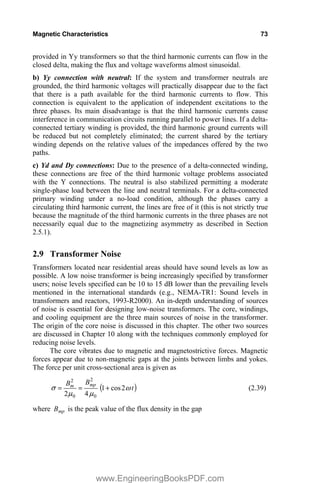
Figure 2.1 (f) shows a typical 3-phase shell-type construction.
2.1.2 Analysis of overlapping joints and the building factor
While building a core, the laminations are placed in such a way that the gaps
between the laminations at joints between limbs and yokes are overlapped by the
laminations in the next layer. This is done so that there is no continuous gap at
joints when laminations are stacked one above the other (Figure 2.2). The
overlapping distance is kept around 15 to 20 mm. Two types of joints are shown
in Figure 2.3. Non-mitered joints, in which the overlap angle is 90°, are simple
from the manufacturing point of view, but the loss in their corners is more since
the flux in them is not along the direction in which grains are oriented. Hence,
the non-mitered joints are used for very small transformers. These joints were
commonly adopted in the earlier days when non-oriented materials were
commonly used even for larger transformers.
In mitered joints, the angle of overlap )
(D is of the order of 30° to 60°;
the most commonly used angle is 45°. The flux crosses at the joints along the
direction of the grain orientation, minimizing losses in them. For air-gaps of
equal length, the excitation requirement with mitered joints is D
sin times that
with non-mitered joints [5].
overlap
A
A
(a) Overlap at corner (b) Cross section A-A
Figure 2.2 Overlapping at joints.
www.EngineeringBooksPDF.com](https://image.slidesharecdn.com/transformer-engineering-design-technology-and-diagnostics-second-edition-pdf-230506172819-680afe24/85/transformer-engineering-design-technology-and-diagnostics-second-edition-pdf-pdf-62-320.jpg)
![42 Chapter 2
Non-mitered joint Mitered joint
Figure 2.3 Commonly used joints.
Better grades (Hi-B, scribed, etc.) having specific loss (watts/kg) about 15
to 20% lower than conventional CRGO materials (termed hereafter as CGO
grades, e.g., M4) are regularly used. However, it is generally observed that the
use of these better grades may not give expected loss reductions if a proper
value of building factor is not used in loss calculations. The factor is defined as
)
/
(
)
/
(
kg
watts
loss
core
Epstein
Material
kg
watts
loss
core
r
transforme
Built
factor
Building . (2.1)
The building factor increases with the quality of the grade from CGO to
Hi-B to scribed (domain refined). This is because of the fact that the penalties
for deviations of flux, at the joints, away from the direction of the grain
orientation are higher for the better grades. The factor is also a function of the
operating flux density; it usually deteriorates rapidly for the better grades at
higher flux densities. Hence, the cores built with better grades may not give
expected benefits in line with Epstein measurements done on a single lamination
sheet. Therefore, appropriate building factors should be used based on
experimental /test data.
Single-phase two-limb transformers give significantly better performances
than three-phase cores; the building factor can be as low as 1.0 for the domain-
refined grades and even less than 1.0 for the CGO grades [6]. The lower values
of losses are due to lightly loaded joints and spatial redistributions of flux in the
limbs and yokes across the width of the laminations. Needless to say, the higher
the proportion of the weight of the joints in the total core weight the higher the
losses are. Also the loss contribution due to the joints is higher with 90° joints as
compared to that with 45° joints since there is over-crowding of flux lines at the
inner edge and the flux is not along the direction of the grain orientation while
passing from the limb to the yoke in the former case. The smaller the
overlapping length the better the core performance is; but the improvement may
not be noticeable. It is also reported in [6, 7] that the gap at the core joint has a
significant impact on the no-load loss and current. As compared to 0 mm gap,
the increase in loss is 1 to 2% for 1.5 mm gap, 3 to 4% for 2.0 mm gap, and 8 to
12% for 3 mm gap. These figures highlight the need for maintaining minimum
gaps at the core joints.
www.EngineeringBooksPDF.com](https://image.slidesharecdn.com/transformer-engineering-design-technology-and-diagnostics-second-edition-pdf-230506172819-680afe24/85/transformer-engineering-design-technology-and-diagnostics-second-edition-pdf-pdf-63-320.jpg)
![Magnetic Characteristics 43
The lesser the laminations per lay the lower the core loss is. Experience
shows that the constructions with 2 laminations per lay give loss advantage of 3
to 4% as compared to those with 4 laminations per lay. Advantage of 2 to 3% is
further achieved when only 1 lamination per lay is used. As the number of
laminations per lay reduces, the manufacturing time for core building increases.
Hence, the construction with 2 laminations per lay is commonly used.
Analyses of various factors affecting the core loss have been adequately
reported in the related literature. A core model based on a lumped circuit
approximation is elaborated in [8] for three-phase three-limb transformers. The
length of equivalent air gap is varied as a function of the instantaneous value of
the flux in the laminations. Anisotropic material properties are also taken into
account in the model. An analytical formulation based on the finite difference
method is used in [9] to calculate the spatial flux distribution and core loss. The
method takes into account the magnetic anisotropy and nonlinearity. The effects
of overlapping lengths and the number of laminations per lay on the core loss
have been analyzed in [10] for wound core distribution transformers.
Joints between limbs and yokes contribute significantly to the core loss
due to cross-fluxing and crowding of flux lines in them. Hence, a higher
proportion of the weight of the joints in the total weight leads to an increased
loss. Due to lower cross-sectional areas as compared to the main limb area, the
weight of the joints in single-phase three-limb, single-phase four-limb and three-
phase five-limb constructions is less. However, the corresponding benefit in the
core loss is negated by an increased overall weight (due to additional end limbs
and yokes).
The building factor is usually in the range of 1.1 to 1.25 for three-phase
three-limb cores with mitered joints. A higher height-to-width ratio of the core
windows results in a decreased proportion of the weight of the joints; the core
loss decreases giving a lower value of the building factor. Single-phase two-limb
and single-phase three-limb cores have been shown [11] to have fairly uniform
flux distributions and lower levels of total harmonic distortions as compared to
single-phase four-limb and three-phase five-limb cores.
Step-lap joints are replacing mitered joints due to their superior
performance [12, 13]. A typical step-lap joint consists of a group of laminations
(normally 5 to 7) stacked with a staggered joint as shown in Figure 2.4.
Step-lap joint Conventional mitered joint
Figure 2.4 Step-lap and conventional joints.
www.EngineeringBooksPDF.com](https://image.slidesharecdn.com/transformer-engineering-design-technology-and-diagnostics-second-edition-pdf-230506172819-680afe24/85/transformer-engineering-design-technology-and-diagnostics-second-edition-pdf-pdf-64-320.jpg)
![44 Chapter 2
It is shown in [13] that, for an operating flux density of 1.7 T, the flux density
in the mitered joint in the core sheet area shunting the air gap rises to 2.7 T
(heavy saturation), while in the gap the flux density is about 0.7 T. Contrary to
this, in the step-lap joint with 6 steps, the flux almost avoids the gap in which
the observed flux density value is just 0.04 T; the flux gets redistributed just
about equally in the laminations of the other five steps with a flux density close
to 2.0 T in them. This explains why there is a marked improvement in the no-
load performance figures (current, loss and noise) in the constructions with step-
lap joints.
2.2 Hysteresis, Eddy, and Anomalous Losses
2.2.1 Classical theory
Hysteresis and eddy current losses together constitute the no-load loss according
to the classical theory. As discussed in Chapter 1, the loss due to the no-load
current flowing in the primary winding is negligible. Also, at the rated flux
density condition on no-load, since most of the flux is confined to the core,
negligible losses are produced in the structural parts due to near absence of stray
flux. The hysteresis and eddy losses arise due to successive reversals of the
magnetization in the iron core excited by a sinusoidal voltage source at a
particular frequency f (cycles/second).
The eddy loss, occurring on account of eddy currents produced due to
induced voltages in laminations in response to an alternating flux, is
proportional to the square of the thickness of laminations, the square of the
frequency and the square of the effective (r.m.s.) value of the flux density.
The hysteresis loss is proportional to the area of the hysteresis loop; a
typical loop is shown in Figure 2.5(a).
Bm
000
000
111
111
000
111
A
E
G
I
F
C
D
O
m
i
,
o
B
H
,
0
a. Hysteresis loop b. Waveforms
Figure 2.5 Hysteresis loss.
m
I e
0
i
m
i
h
i
E
t
www.EngineeringBooksPDF.com](https://image.slidesharecdn.com/transformer-engineering-design-technology-and-diagnostics-second-edition-pdf-230506172819-680afe24/85/transformer-engineering-design-technology-and-diagnostics-second-edition-pdf-pdf-65-320.jpg)

![46 Chapter 2
determined or an empirical factor is derived for accounting the effect of the
weight at the joints separately:
w
K
W
loss
load
No b
t u
u (2.5)
or c
c
c
t K
w
W
w
W
W
loss
load
No u
u
u
)
( (2.6)
where,
w is watts/kg for a particular operating peak flux density as given by the
supplier (Epstein core loss for a single lamination),
Kb is the building factor,
Wc denotes the weight of the joints out of the total weight of t
W , and
Kc represents the extra loss occurring at the joints (whose value is higher
for smaller core diameters).
2.2.2 Inclusion of anomalous loss
As discussed earlier, the core loss in transformers is usually classified into two
components, viz. the eddy loss and the hysteresis loss, according to the classical
theory. The hysteresis loss is due to the irreversible nature of the magnetic charac-
teristics (B-H curves) when H is repeatedly cycled between –Hm to +Hm as ex-
plained earlier The eddy loss arises due to induced voltages on account of a chang-
ing magnetic induction B; the voltages lead to currents circulating in closed loops.
These eddy currents cause a resistive loss.
The core losses can be calculated by simple formulae given by Equations
2.3 and 2.4 which assume a non-domain structure of the material. They also
assume sinusoidal variation of B. Therefore, the classical theory tends to under-
estimate the core loss. The difference between the measured core loss and the
calculated hysteresis loss is the apparent eddy loss, and the difference between
the apparent and classical eddy loss values is the anomalous loss. In the grain-
oriented transformer steel under normal working conditions, the anomalous loss
can be about one-half of the total core loss [14].
Many efforts have been made in the literature for describing the three com-
ponents of the core loss using a theory based on magnetic domains. A change in
magnetization of the core material occurs because of the motion of the domain
walls and the rotation of the domain magnetization. The hysteresis loss is caused
by the resistance to the domain wall motion due to defects (impurities or disloca-
tions in crystallographic structure) and internal strains in the material. A physical
reasoning for the separation of the core loss into the three components is explained
using a statistical loss theory in [15].
Hysteresis loss: This loss corresponds to the area enclosed by the DC hysteresis
loop. It represents the energy expenditure per cycle of the loop as discussed ear-
lier. Imperfections in the material cause an increase in the energy expenditure
during the magnetization process, in the form of a kind of internal friction to the
www.EngineeringBooksPDF.com](https://image.slidesharecdn.com/transformer-engineering-design-technology-and-diagnostics-second-edition-pdf-230506172819-680afe24/85/transformer-engineering-design-technology-and-diagnostics-second-edition-pdf-pdf-67-320.jpg)
![Magnetic Characteristics 47
domain wall motion. A numerical implementation of the hysteresis model based
on the domain theory is discussed in Section 12.7.6.
Eddy losses: The eddy loss in a lamination can be calculated using the classical
theory which assumes uniform flux throughout its thickness. According to the
theory, the instantaneous eddy loss per unit volume is expressed in terms of the
rms value of the flux density (B) as
2
2
12
E
d dB
P
dt
U
§ ·
¨ ¸
© ¹
(2.7)
where d indicates the thickness of a single lamination and U is the resistivity of
its material. When the magnetic induction B is sinusoidally varying, d dt is
replaced by jZ and the above expression becomes numerically equal to that in
Equation 4.94 with 0 2
B B ,
2
0
E e
P k f B (2.8)
where, 2 2
6
e
k d
S U . The above expression is of the same form as Equation
2.3. Thus, the classical eddy currents are proportional to the square of the
thickness of the lamination and to the square of the frequency of supply. The loss
is inversely proportional to resistivity of the material.
Anomalous loss or microscopic eddy current loss: The measured power losses
for ferromagnetic materials are usually two or three times the value calculated
by using the classical eddy current theory [16]. This problem is referred to as the
eddy current anomaly. Several attempts to explain this anomaly are based on
non-uniform magnetization in the core materials due to the presence of magnetic
domains. The model proposed in [17] has been frequently used in the literature
for interpreting anomalous losses. It assumes an infinite lamination containing a
periodic array of longitudinal domains and calculates the eddy current loss using
Maxwell's equations. The model gives an excess loss in terms of microscopic
eddy currents associated with the domain wall motion. The discrepancies be-
tween the losses given by the model and measurements have been related to
effects such as the presence of irregularities in the wall motion, domain multi-
plications, and wall bowing [18].
A statistical approach has been found to give reasonably accurate results.
The anomalous loss results from the domain wall motion, which can be expressed
as [15]
1 3
2 2
0
A GdbH
dW dB
dt dt
U
§ · § ·
¨ ¸ ¨ ¸
© ¹
© ¹
(2.9)
www.EngineeringBooksPDF.com](https://image.slidesharecdn.com/transformer-engineering-design-technology-and-diagnostics-second-edition-pdf-230506172819-680afe24/85/transformer-engineering-design-technology-and-diagnostics-second-edition-pdf-pdf-68-320.jpg)


![Magnetic Characteristics 51
The core is likely to get saturated under most of the over-excitation
conditions. The spill-over flux from it returns through a predominantly high
reluctance path. The over-excitation must be extreme and of a sufficiently long
duration to produce damaging effects in the core laminations which can
withstand temperatures of about 800 °C (they are annealed at this temperature
during their manufacture), but the insulation in their vicinity, viz. press-board
insulation (class A: 105 °C) and core bolt insulation (class B: 130 °C), may get
damaged. Since the spill-over flux flows only during the part of each cycle when
the core is saturated, it is in the form of pulses with a higher harmonic content
which increases the eddy loss and temperature rise in the windings and structural
parts. Guidelines for permissible short-time over-excitations of transformers are
given in [19, 20]. Generator transformers are more susceptible to overvoltages
due to over-speeding of generators due to load rejection conditions.
2.5 No-Load Loss Test
The hysteresis loss is a function of the average voltage or maximum flux
density, whereas the eddy loss is a function of the r.m.s. voltage or r.m.s. flux
density. Hence, the total core loss is a function of the voltage wave-shape. If the
sine-wave excitation cannot be ensured during the test, the following correction
procedure can be applied to derive the value of no-load loss on the sine wave
basis [21, 22]. When a voltmeter corresponding to the mean value is used, the
reading is proportional to the maximum value of the flux density in the core.
Hence, if the applied non-sinusoidal voltage has the same maximum flux density
as that of the desired sine-wave voltage, the hysteresis loss will be measured
corresponding to the sine wave. Its r.m.s. value may not be equal to the r.m.s.
value of the sine wave, hence the eddy loss has to be corrected by using a factor,
2
2
(actual r.m.s. voltage of the applied voltage)
(r.m.s. voltage on the sine wave basis)
e
K .
The true core loss of the transformer ( c
P ) on the sine wave basis is then
calculated from the measured loss ( m
P ) as
'
'
e
e
h
m
c
P
K
P
P
P
(2.12)
where '
h
P and '
e
P are the hysteresis and eddy loss fractions of the total core loss,
respectively. The following values are usually taken for these two fractions,
5
.
0
'
h
P and 5
.
0
'
e
P for cold rolled steel
7
.
0
'
h
P and 3
.
0
'
e
P for hot rolled steel
www.EngineeringBooksPDF.com](https://image.slidesharecdn.com/transformer-engineering-design-technology-and-diagnostics-second-edition-pdf-230506172819-680afe24/85/transformer-engineering-design-technology-and-diagnostics-second-edition-pdf-pdf-72-320.jpg)
![52 Chapter 2
The calculation according to Equation 2.12 is recommended in ANSI Standard
C57.12.90-1999. For highly distorted waveforms (with multiple zero crossings
per period), a correction which can be applied to this equation is given in [23].
According to IEC 60076-1 (Edition 2.1, 2000), the test voltage has to be
adjusted according to a voltmeter responsive to the mean value of the voltage
but scaled to read the r.m.s. voltage of a sinusoidal wave having the same mean
value. Let the reading of this voltmeter be 1
V . At the same time, a voltmeter
responsive to the r.m.s. value of the voltage is connected in parallel with the
mean value voltmeter, and let its reading be V. The wave shape of the test
voltage is satisfactory if the readings 1
V and V are within 3% of each other. If
the measured no-load loss is m
P then the corrected no-load loss ( c
P ) is given as
d
P
P m
c
1 (2.13)
where
1
1
V
V
V
d
(usually negative)
The method given in [24] allows the determination of the core loss from the
measured data under a non-sinusoidal excitation without an artificial separation
of the hysteresis and eddy losses. Harmonic components are taken into account.
The computed results have been compared with the IEC method.
A voltage regulator with a large capacitor bank is better than a conventional
rotating machine source from the point of view of obtaining as sinusoidal
voltage as possible for core loss measurements.
The no-load loss test and the calculation of shunt parameters of the
equivalent circuit have been elaborated in Chapter 1. Now, special topics/case
studies related to the no-load test are discussed.
2.5.1 Asymmetrical magnetizing phenomenon
Unlike in a bank of three single-phase transformers having independent
magnetic circuits, the different phases are wound on a common magnetic circuit
in the three-phase three-limb construction. The excitation currents and powers
drawn by the three phases are not the real requirements by the corresponding
magnetic sections of the core. The current drawn by each phase winding is a
function of the requirements of all the three phases. Consider a three-phase
three-limb core shown in Figure 2.7. Let the magnetomotive forces required to
produce instantaneous values of fluxes ( r
I , y
I and b
I ) in the path between
points P1 to P2 for the phase windings ( r , y and b ) be '
r
NI , '
y
NI and '
b
NI ,
respectively. There is an inherent asymmetry in the core as the length of
magnetic path between the points P1 and P2 for y phase is less than that for the
phases r and b . Let the currents drawn from the supply be r
I , y
I and b
I .
www.EngineeringBooksPDF.com](https://image.slidesharecdn.com/transformer-engineering-design-technology-and-diagnostics-second-edition-pdf-230506172819-680afe24/85/transformer-engineering-design-technology-and-diagnostics-second-edition-pdf-pdf-73-320.jpg)

![54 Chapter 2
core between the points P1 and P2 [25]. The magnitude of this flux is quite small
as compared to the mutual flux in the core. For convenience, the reluctance of
the magnetic path for the phase y between P1 and P2 is taken as half of that for
the extreme phases ( r and b). For a sinusoidal three-phase applied voltage, the
established mutual flux is also sinusoidal, and the required excitation currents
contain harmonics as explained earlier. Therefore, the currents in the three-
phases can be expressed as (with higher order harmonics neglected)
t
I
t
I
t
I
I c
r Z
Z
Z 3
sin
sin
cos 3
1
'
(2.22)
)
120
(
3
sin
5
.
0
)
120
sin(
5
.
0
)
120
cos(
5
.
0 0
3
0
1
0
'
t
I
t
I
t
I
I c
y Z
Z
Z
(2.23)
)
240
(
3
sin
)
240
sin(
)
240
cos( 0
3
0
1
0
'
t
I
t
I
t
I
I c
b Z
Z
Z (2.24)
where c
I is the core loss component, and a negative sign is taken for the third
harmonic components [26] to obtain a peaky nature of the excitation current (for
a sinusoidal flux, the excitation current is peaky in nature due to nonlinear
magnetic characteristics). Substituting these expressions in Equation 2.21,
)
3
sin(
833
.
0
)
60
sin(
167
.
0
)
60
cos(
167
.
0 3
0
1
0
t
I
t
I
t
I
I c
z Z
Z
Z
.
(2.25)
After substituting this expression of z
I and the expressions of '
y
'
r I
,
I and '
b
I
from Equations 2.22 to 2.24 in Equations 2.18 to 2.20, the excitation currents
drawn from the source are
)
3
sin(
167
.
0
)
9
sin(
928
.
0
)
9
cos(
928
.
0 3
0
1
0
t
I
t
I
t
I
I c
r Z
Z
Z
(2.26)
)
3
sin(
333
.
0
)
120
sin(
667
.
0
)
120
cos(
667
.
0 3
0
1
0
t
I
t
I
t
I
I c
y Z
Z
Z
(2.27)
)
3
sin(
167
.
0
)
129
sin(
928
.
0
)
129
cos(
928
.
0 3
0
1
0
t
I
t
I
t
I
I c
b Z
Z
Z
.
(2.28)
Since the neutral is isolated, the sum of the 3rd
harmonic currents in three
phases has to be zero; this condition is satisfied by the above three equations.
The essence of the mathematical treatment can be understood by the vector
diagrams of the fundamental and third harmonic components shown in Figure
2.8. The magnitudes of r
I and b
I are almost equal and these are greater than
the magnitude of y
I . The current y
I , though smallest of all the three currents, is
higher than the current required to excite the middle phase alone ( '
y
y I
I ! ). The
currents in the outer phases are slightly less than that needed to excite the outer
limbs alone ( '
r
r I
I and '
b
b I
I ). In actual practice, the currents r
I and b
I
www.EngineeringBooksPDF.com](https://image.slidesharecdn.com/transformer-engineering-design-technology-and-diagnostics-second-edition-pdf-230506172819-680afe24/85/transformer-engineering-design-technology-and-diagnostics-second-edition-pdf-pdf-75-320.jpg)
![Magnetic Characteristics 55
may differ slightly due to minor differences in the characteristics of magnetic
paths (e.g., unequal air gap lengths at joints). The third harmonic component
drawn by the y phase is greater than that of the r and b phases.
Since the applied voltage is assumed to be sinusoidal, only the
fundamental component contributes to the power. The wattmeter of the r phase
reads negative if z
I is large enough to cause the angle between r
V and r
I to
exceed 90°. A negative power value is measured in one of the phases during the
no-load loss test when yoke lengths are comparable to limb heights increasing
the asymmetry between the middle and outer phases.
It has been proved in [27] that when the reluctance of the central phase is
half that of the outer phases,
1
:
718
.
0
:
1
:
: b
y
r I
I
I . (2.29)
The effect of change in the excitation is illustrated for the r phase in Figure
2.9. The no-load test is usually carried out at 90%, 100% and 110% of the rated
voltage. The magnetizing component of the excitation current is more sensitive
to an increase in flux density as compared to the core loss component.
Consequently as the voltage is increased, the no-load power factor decreases.
The value of z
I also increases, and hence the possibility of the negative power
phenomenon increases with an increase in the applied voltage. When the angle
between Vr and Ir is 90°, the r phase wattmeter reads zero, and if it exceeds 90°
the wattmeter reads negative.
Iy
I '
y
-Iz
-Iz
-Iz
'+ I '+ I ')
V
I
I '
I
I '
I
r
r
r
z
(Ir y
b
b
b
a. Fundamental components b. Third harmonic components
Figure 2.8 Magnetizing asymmetry.
I3
I3
2
5 I3
6
I3
3
I3
6
I3
6
I' I' I
I3
I I
I'
r y z r
b b Iy
www.EngineeringBooksPDF.com](https://image.slidesharecdn.com/transformer-engineering-design-technology-and-diagnostics-second-edition-pdf-230506172819-680afe24/85/transformer-engineering-design-technology-and-diagnostics-second-edition-pdf-pdf-76-320.jpg)
![56 Chapter 2
Vr
I
'
I '
'
I
-I -I
-I
I
r
r
r
r
r
I
90%
100% 110%
z z z
Figure 2.9 Effect of excitation level.
The magnetizing asymmetry phenomenon described above has been
analyzed by using mutual impedances between three phases in [28]. It is shown
that phase currents and powers are balanced if mutual impedances yb
ry Z
,
Z and
br
Z are equal. These impedances depend on the number of turns and disposition
of windings, their connections, and more importantly on the dimensions and
layout of the core. Because of the unbalanced mutual impedances in the three-
phase three-limb construction ( br
yb
ry Z
Z
Z z ), the total no-load power is
redistributed between the three phases. The form of asymmetry occurring in the
phase currents and powers is different for the three-limb and five-limb
constructions. It is reported in [28] that there is star point displacement in the
five-limb transformers, which tends to reduce the unbalance caused by the
inequality of the mutual impedances.
If the primary winding is delta-connected, a similar analysis can be
performed for which a measured line current is the difference between the
currents of the corresponding two phases. It can be proved that when the delta-
connected winding is energized, for the Yd1 or Dy11 connection, the line
current drawn by the r phase is higher than the currents drawn by the y and b
phases, which are equal ( L
b
L
y
L
r I
I
I
! ) [29]. For the Yd11 or Dy1
connection, the line current drawn by the b phase is higher than the currents
drawn by the r and y phases, which are equal ( L
r
L
y
L
b I
I
I
! ). It should
be noted that, for the delta connected primary winding also, the magnetic section
corresponding to the y phase requires the least magnetizing current, i.e.,
( '
b
'
r
'
y I
,
I
I ), but the phasor additions of the phase currents results into a
condition in which L
y
I equals the line current of one of the outer phases.
www.EngineeringBooksPDF.com](https://image.slidesharecdn.com/transformer-engineering-design-technology-and-diagnostics-second-edition-pdf-230506172819-680afe24/85/transformer-engineering-design-technology-and-diagnostics-second-edition-pdf-pdf-77-320.jpg)

![58 Chapter 2
fault, parallel conductors are electrically separated at both ends, and then
resistance values are measured between all the points available ( '
,
,
'
,
,
'
, 3
3
2
2
1
1 )
as shown in Figure 2.10; the winding is assumed to have 3 parallel conductors
per turn.
Let us assume that each of the parallel conductors is having a resistance of
0.6 ohms. If the fault is at a location 70% from the winding bottom between
conductor 1 of one turn and conductor 3 of the next turn, the measured values of
resistances between 3
1 and '
' 3
1 will be 0.36 ohms (2 u 0.3u 0.6) and 0.84
ohms (2u 0.7u 0.6), respectively. The voltage corresponding to one turn
circulates very high currents since these are limited only by the above
resistances; the reactance of individual conductors is very small. An increase in
the no-load loss value corresponds approximately to the loss in these two
resistive paths due to the induced circulating currents.
2.5.4 Effect of impulse test on no-load loss
A slight increase of about few % in the no-load loss value is sometimes
observed after impulse tests due to partial breakdowns of interlamination
insulations (particularly at edges) resulting into an increased eddy loss. The
phenomenon has been analyzed in [30], wherein it is reported that voltages are
induced in the core by electrostatic as well as electromagnetic inductions. A loss
increase to the tune of 2% is possible. The phenomenon is harmful to the extent
that it increases the loss which, however, may not increase further in field.
Application of an adhesive at the edges can prevent partial and localized
damages to the core during the high voltage test.
2.6 Impact of Manufacturing Processes
For building cores of various ratings of transformers, different lamination widths
are required. Since lamination rolls are available in some standard widths from
suppliers, slitting operations are inevitable. It is obvious that in most cases full
widths cannot be utilized and the scrap of the leftover material has to be
minimized by a meticulous planning exercise. A manufacturer having a wide
product range can use the leftover pieces of the cores of large transformers for
the cores of small distribution transformers.
+1
turn
N
1' '
2 '
3
1
2
3
fault
2
1
3
2 3
. .
turn
N
1
fault 70%
turn turn +1
N N
Figure 2.10 Troubleshooting during no-load loss test.
www.EngineeringBooksPDF.com](https://image.slidesharecdn.com/transformer-engineering-design-technology-and-diagnostics-second-edition-pdf-230506172819-680afe24/85/transformer-engineering-design-technology-and-diagnostics-second-edition-pdf-pdf-79-320.jpg)


![62 Chapter 2
Figure 2.14 Typical inrush current waveform.
)
cos(
)
cos
( 1
1
T
Z
I
I
T
I
I
r
t
t
e mp
L
R
r
mp
m . (2.31)
For 0
T and the residual flux of r
I
, the waveform of flux (flux density) is
shown in Figure 2.13. It can be observed from Equation 2.31 that the flux
waveform has a transient DC component which decays at a rate determined by
the time constant of the primary winding (i.e., 1 1
/
L R ), and a steady-state AC
component viz. cos( ).
mp t
I Z T
A typical inrush current waveform is shown in
Figure 2.14 for a phase switched on at the most unfavourable instant (i.e., at zero
crossing of the applied voltage wave).
It can be observed that the current waveform is completely offset in the
first few cycles with the wiping out of alternate half cycles because the flux
density is below the saturation value for these half cycles, resulting in very small
current values. Hence, the inrush current is highly asymmetrical and has a
predominant second harmonic component which is used by differential
protection schemes to restrain relays from operating.
In practice the time constant (L/R) of the circuit is not constant; the value
of L changes with the flux density value. During the first few cycles, the core
can be in a deep saturation state and therefore L is small. Hence, the initial rate
of the decay of the inrush current is high. As the winding and core losses damp
the circuit and the flux density falls, L increases slowing down the decay. Hence,
the decay starts with a high initial rate which progressively reduces; the total
phenomenon lasts for a few seconds. Smaller transformers have higher decay
rates because of smaller time constants. In general, inrush currents in less
efficient (high loss) transformers have high decay rates [31].
While deriving Equation 2.31, linear magnetic characteristics are assumed,
which is a major approximation. Accurate procedures for the calculation of
inrush currents in single-phase transformers is given in the literature [32, 33] in
which nonlinear magnetic characteristics are elaborately represented. For three-
phase transformers, the analysis is more involved [34, 35, 36]. Inrush currents
can be calculated in the harmonic domain for single-phase and three-phase
transformers using operational matrices as given in [37]. Overvoltages in HVDC
systems following inrush current transients are dealt in [38], wherein an
inductive AC system impedance, due to generators, transformers and
transmission lines, is shown to resonate with filters. If the resulting resonance
frequency of the combination is equal to or close to a harmonic component of
the inrush current of the same frequency, overvoltages occur.
www.EngineeringBooksPDF.com](https://image.slidesharecdn.com/transformer-engineering-design-technology-and-diagnostics-second-edition-pdf-230506172819-680afe24/85/transformer-engineering-design-technology-and-diagnostics-second-edition-pdf-pdf-83-320.jpg)

![64 Chapter 2
( max
0
i ) of the single-phase transformer is shown in Figure 2.15. It is assumed
that the phase a has the maximum transient inrush current.
Since the delta allows the flow of zero-sequence currents, it holds the
neutral voltage at a stable value and maintains normal line-to-neutral voltages
across the phases. The presence of the delta also ensures the full single-phase
transient in the phase that has maximum inrush current (the phase a in this
case). Two-thirds of the required single-phase inrush current )
3
2
( max
0
i flow in
the phase a on the star side and the remaining one-third flows on the delta side.
Hence, the maximum inrush current in this case is 2 3 times that of the single-
phase transformer. The phases b and c do not get magnetized since the currents
in them are equal and opposite on the star and delta sides.
3) A three-phase three-limb transformer (in which the phases are magnetically
interlinked) can be treated as consisting of three independent single-phase
transformers [22, 34] under inrush transients; for a star-connected primary
winding, the inrush phenomenon is similar to that of Case 2, irrespective of
whether the secondary winding is star- or delta-connected. Maximum inrush
current is approximately equal to two-thirds of that corresponding to the single-
phase operation.
2.7.3 Estimation of decay pattern
Equation 2.34 is an approximate formula giving maximum possible inrush
current. Practicing engineers may be interested in knowing inrush current peak
values for the first few cycles or the time after which the inrush current reduces
to a value equal to the rated current. The procedures for estimating inrush
current peaks for first few cycles are given in [39, 40]. The procedures are
generally applicable for a few tens of initial cycles.
3
a
b
c
B
A
C
2i0max
3
i
3
i
0max 0max
3
i0max
Figure 2.15 Inrush in a star-delta bank of transformers.
www.EngineeringBooksPDF.com](https://image.slidesharecdn.com/transformer-engineering-design-technology-and-diagnostics-second-edition-pdf-230506172819-680afe24/85/transformer-engineering-design-technology-and-diagnostics-second-edition-pdf-pdf-85-320.jpg)
![Magnetic Characteristics 65
Example 2.1
Calculate inrush current peaks for the first 5 cycles for a 31.5 MVA, 132/33 kV,
50 Hz, Yd1 transformer, when energized from its 132 kV winding having 920
turns, mean diameter of 980 mm and height of 1250 mm. The peak operating
flux density is 1.7 T for the core area of 0.22 m2
. The sum of system and
winding resistances is 0.9 ohms.
Solution:
The transformer is assumed to be energized at an instant when the applied
voltage to one of the phases is at zero value and increasing. It is also assumed
that the residual flux is in the same direction as that of the initial flux change,
thus giving maximum possible value of the inrush current. After the core
saturates, the inrush current is limited by the air core reactance of the excited
winding, s
X , which can be calculated using a standard formula.
Step 1:
f
h
A
N
X
w
w
s u
u
u S
P
2
2
0
(2.35)
N = number of turns of the excited winding = 920 turns
w
A area inside the mean turn of the excited winding
= 2
)
(
4
diameter
mean
S
= 754
.
0
)
980
.
0
(
4
2
S
m2
w
h height of the excited winding = 1.25 m
50
2
25
.
1
754
.
0
920
10
4 2
7
u
u
u
u
u
u
?
S
S
s
X = 202 ohms.
Step 2:
Now angle T is calculated [39], which corresponds to the instant at which the
core saturates,
°
¿
°
¾
½
°̄
°
®
mp
r
mp
s
B
B
B
B
K 1
1 cos
T (2.36)
where Bs is the saturation flux density = 2.03 T
Bmp is the peak value of the operating flux density in the core = 1.7 T
Br is the residual flux density = 0.8 u Bmp = 1.36 T
(For cold rolled materials, the maximum residual flux density can be
taken as 80% of the rated peak flux density, whereas for hot rolled
materials it can be taken as 60% of the rated peak flux density.)
www.EngineeringBooksPDF.com](https://image.slidesharecdn.com/transformer-engineering-design-technology-and-diagnostics-second-edition-pdf-230506172819-680afe24/85/transformer-engineering-design-technology-and-diagnostics-second-edition-pdf-pdf-86-320.jpg)
![66 Chapter 2
K1 = correction factor for the saturation angle = 0.9
0
.
2
7
.
1
36
.
1
7
.
1
03
.
2
cos
9
.
0 1
¿
¾
½
¯
®
u
?
T radians.
Step 3:
The inrush current peak for the first cycle is calculated as [39],
T
cos
1
2
2
max
0
s
X
V
K
i (2.37)
where V is the r.m.s. value of the applied alternating voltage
2
K is a correction factor for the peak value = 1.15
869
0
.
2
cos
1
202
2
)
3
132000
(
15
.
1
max
0
u
?i amperes.
The current calculated by Equation 2.34, for the core area of 0.22 m2
, is
861
920
754
.
0
10
4
25
.
1
22
.
0
)
03
.
2
36
.
1
7
.
1
2
(
7
max
0
u
u
u
u
u
u
S
i amperes,
which is very close to that calculated by the more accurate method.
Step 4:
After having calculated the value of inrush current peak for the first cycle, the
residual flux density at the end of the first cycle is calculated. The residual
component of the flux density reduces due to losses in the circuit, and hence it is
a function of damping provided by the losses in the transformer. The new value
of the residual flux density can be calculated as [39]
@
)
cos
(sin
2
)
(
)
( 3
T
T
T
u
s
mp
r
r
X
R
K
B
old
B
new
B (2.38)
where R = sum of the transformer winding resistance and the system resistance
= 0.9 ohms
3
K = correction factor for the decay of inrush = 2.26
@
2.26×0.9
1.36 1.7× 2(sin2.0 2.0cos2.0) =1.3
202
( )
r
B new
? T
Steps 2, 3 and 4 are repeated to calculate the peaks of subsequent cycles. The
inrush current peaks for the first 5 cycles are 869 A, 846 A, 825 A, 805 A and
786 A on the single-phase basis. Since it is a star-delta connected three-phase
three-limb transformer, actual line currents are approximately two-thirds of
these values (579 A, 564 A, 550 A, 537 A and 524 A).
www.EngineeringBooksPDF.com](https://image.slidesharecdn.com/transformer-engineering-design-technology-and-diagnostics-second-edition-pdf-230506172819-680afe24/85/transformer-engineering-design-technology-and-diagnostics-second-edition-pdf-pdf-87-320.jpg)
![Magnetic Characteristics 67
The inrush current phenomenon may not be harmful to the transformer
(although repeated switching on and off in a short period of time is not
advisable). The behavior of transformers under inrush conditions continues to
attract attention of researchers. The differences in forces acting on the windings
during the inrush and short-circuit conditions are enumerated in [41]. An inrush
current may result in the inadvertent operation of overload and differential
relays, tripping the transformer out of the circuit as soon as it is switched on.
Relays that discriminate between inrush and fault conditions are used:
1) Since inrush currents have a predominant second harmonic component,
differential relays with a second harmonic restraint are used to prevent their mal-
operation.
2) Differential relays with higher pick-ups can be used to reduce their sensitivity
to asymmetrical waves; furthermore, a time delay can be added to override high
initial peaks.
A technique for discriminating inrush currents from internal fault currents
is described in [42]; it uses a combination of the wavelet transform and neural
network approaches. The ability of the wavelet transform to extract the required
information from transient signals simultaneously in the time and frequency
domains is exploited for the purpose. High inrush currents may cause excessive
momentary dips in system voltages affecting operations of various electrical
equipment. A switching-on operation of a transformer in an interconnected
network can affect already energized transformers as explained below.
2.7.4 Sympathetic inrush phenomenon
It has long been known that transient magnetizing inrush currents, sometimes
reaching magnitudes as high as six to eight times the rated currents, can flow in
transformers during their energization. It is generally not appreciated, however,
that the other transformers, already connected to the network near the
transformer being switched, may also have a transient magnetizing current of an
appreciable magnitude at the same time. In order to understand how energizing
of a transformer affects the operating conditions of the other interconnected
transformers, consider a network as shown in Figure 2.16.
Transmission line A
C
B
Source
Figure 2.16 Sympathetic inrush.
www.EngineeringBooksPDF.com](https://image.slidesharecdn.com/transformer-engineering-design-technology-and-diagnostics-second-edition-pdf-230506172819-680afe24/85/transformer-engineering-design-technology-and-diagnostics-second-edition-pdf-pdf-88-320.jpg)
![68 Chapter 2
When transformer B is switched on to the network already feeding similar
transformers (C) in its neighborhood, the transient magnetizing inrush current of
the switched-on transformer also flows into these other transformers and
produces in them a DC flux which is superimposed on their normal AC
magnetizing flux. This gives rise to increased flux density values and higher
magnetizing currents in them [22, 43, 44]. These sympathetic inrush currents are
substantially less than their usual inrush currents. Depending on the magnitude
of the decaying DC component, this sympathetic (indirect) inrush phenomenon
leads to increased noise levels in these connected transformers due to a higher
flux density value in the core for the transient period. It may also lead to mal-
operations of protective equipment. An increase in the noise level of an
upstream power transformer during the energization of a downstream
distribution transformer (fed by the power transformer) has been analyzed in
[45]; the analysis is supported by noise level measurements carried out during
switching operations.
Let us now analyze the case of parallel transformers shown in Figure 2.17
(a). The transformers may or may not be paralleled on the secondary side. The
DC component of the inrush current of the transformer being energized flows
through the transmission line resistance (between the source and the
transformer) producing a DC voltage drop across it. The voltage drop forces the
core of the already energized transformer towards saturation in a direction
opposite to that of the transformer which is being switched on, resulting in a
buildup of the magnetizing current in it; this rate of the buildup is the same as
the rate at which the DC component of the magnetizing current is decreasing in
the transformer being switched-on. When the two parallel transformers are
similar and the magnitudes of the DC components of the currents in both the
transformers become equal, there is no DC component in the line feeding both
the transformers. However, there is a DC component circulating in the loop
circuit between them, whose rate of decay is very slow due to high inductance
and small resistance values of the windings of the two transformers. The
waveforms of the currents are shown in Figure 2.17 (b).
Since the line current feeding the transformers becomes symmetrical
(waveform Ic) devoid of the second harmonic component, differential relaying
with a second harmonic constraint needs to be provided to each transformer
separately instead of protecting them as a unit [46]. The phenomenon is more
severe when transformers are fed from a weak system (i.e., transformers
connected to a common feeder with a limited fault level and a high internal
resistance). For a further discussion on the phenomenon, refer Section 13.6.
www.EngineeringBooksPDF.com](https://image.slidesharecdn.com/transformer-engineering-design-technology-and-diagnostics-second-edition-pdf-230506172819-680afe24/85/transformer-engineering-design-technology-and-diagnostics-second-edition-pdf-pdf-89-320.jpg)
![Magnetic Characteristics 69
Ic
Ia
Ib
Resistance
Transformer
being energized
already energized
Transformer
Source
(a)
(b)
Figure 2.17 Inrush currents in parallel transformers.
2.7.5 Factors affecting inrush phenomenon
Various factors affecting the inrush current phenomenon are now summarized:
A. Switching-on angle (D )
The inrush current decreases when the switching-on angle (on the voltage wave)
increases. It is maximum for D 0° and minimum for D 90°.
B. Residual flux density
The inrush current is significantly aggravated by the residual flux density which
depends upon core material characteristics and the power factor of the load
when the transformer was switched off. The instant of switching-off has an
effect on the residual flux density depending upon the type of the load [22]. The
total current is made up of the magnetizing current component and the load
current component. The current interruption generally occurs at or near zero of
the total current waveform. The magnetizing current passes through its
maximum value before the instant at which total current is switched-off for no
load, lagging load and unity power factor load conditions, resulting in maximum
value of the residual flux density as per the B-H curve of Figure 2.5. For leading
www.EngineeringBooksPDF.com](https://image.slidesharecdn.com/transformer-engineering-design-technology-and-diagnostics-second-edition-pdf-230506172819-680afe24/85/transformer-engineering-design-technology-and-diagnostics-second-edition-pdf-pdf-90-320.jpg)
![70 Chapter 2
loads, if the leading component is less than the magnetizing component, at zero
of the resultant current the magnetizing component will have reached the
maximum value resulting in maximum residual. On the contrary, if the leading
current component is more than the magnetizing component, the angle between
the peak of the magnetizing current and the zero of the resultant current will be
more than 90°. Hence, at the interruption of the resultant current, the
magnetizing component will not have reached its maximum, resulting in a lower
value of the residual flux density.
The type of the core material also decides the value of the residual flux
density. Its maximum value is usually taken as about 80% and 60% of the
saturation value for the cold-rolled and hot-rolled materials, respectively. It is
also a function of joint characteristics; its values for mitered and step-lap joints
will be different.
C. Series resistance
The resistance of the line between the source and the transformer has a
predominant effect on the inrush phenomenon. The damping effect provided by
the resistance not only reduces the peak initial inrush current but also hastens its
decay rate. Transformers near generators usually have inrush transients lasting
for a long period of time because of a low value of the available resistance.
Similarly, large power transformers tend to have inrush currents with a slow
decay rate since they have a large value of inductance in comparison to the
resistances of their primary winding and the connected system.
Consider a series circuit of two transformers, with T feeding T1, as shown
in Figure 2.18. When transformer T1 is energized, transformer T experiences
sympathetic inrush. The resistance of the line between T and T1 contributes
mainly to the decay of the inrush current of T1 (and T) [47], and not the
resistance on the primary side of T.
For a parallel connection of two transformers (e.g., Figure 2.17), the
sympathetic inrush phenomenon experienced by the transformer already
energized is due to the coupling between the transformers on account of the DC
voltage drop in the transmission line feeding them. Hence, the higher the
transmission line resistance the higher the sympathetic inrush is [48].
T1
T
Transmission line
Figure 2.18 Sympathetic inrush in series connection.
www.EngineeringBooksPDF.com](https://image.slidesharecdn.com/transformer-engineering-design-technology-and-diagnostics-second-edition-pdf-230506172819-680afe24/85/transformer-engineering-design-technology-and-diagnostics-second-edition-pdf-pdf-91-320.jpg)
![Magnetic Characteristics 71
D. Inrush under load
If a transformer is switched on with load, the inrush peaks are affected to some
extent by the load power factor. Under heavy load conditions with the power
factor close to unity, the peak value of the inrush current is lower, and as the
power factor reduces (to either lagging or leading), the peak value is higher [32].
2.7.6 Mitigation of inrush current
Inrush currents in saturated core conditions are limited by the air-core reactance
of the excited windings and hence they are usually lower than the peak short-
circuit currents due to faults. Since transformers are designed to withstand
mechanical effects of short-circuit forces, inrush currents may not be considered
to be dangerous, although they may unnecessarily cause protective equipment
like relays and fuses to operate.
One of the natural ways of reducing inrush currents is to switch-in
transformers through a closing resistor. The applied rated voltage is reduced to a
low value (e.g., 50%) because of the resistor, thus reducing the inrush current.
The resistor is subsequently bypassed to apply the full voltage to the transformer
[38, 49]. Its value should be small enough to allow the passage of the normal
magnetizing current.
If possible, transformers should be switched from their high voltage side; a
higher value of the air core reactance of the outer HV winding (on account of its
larger size) reduces the inrush current.
Since residual flux is one of the main reasons for high inrush currents, any
attempt to reduce it helps in mitigating the phenomenon. When a transformer is
being switched off, if a capacitor of suitable size is connected across it [31], a
damped oscillation will result, causing an alternating current to flow in the
transformer winding. The amplitude of the current decreases with time,
gradually reducing the area of the traversed hysteresis loop, eventually reducing
both the current and the residual flux to zero. For small transformers, a variable
AC source can be used to demagnetize the core. The applied voltage is slowly
reduced to zero for the purpose.
Various schemes for controlled closing at favorable instants have been
proposed in [50]. In these methods, each winding is closed when the prospective
and dynamic (transient) core fluxes are equal, thus, resulting in an optimal
energization without the inrush transients.
2.8 Influence of the Core Construction and Winding
Connections on No-Load Harmonic Phenomenon
The excitation current is a small percentage of the rated current in transformers.
With the increase in rating of transformers, the percentage no-load current
usually reduces. The harmonics in the excitation current may cause interference
www.EngineeringBooksPDF.com](https://image.slidesharecdn.com/transformer-engineering-design-technology-and-diagnostics-second-edition-pdf-230506172819-680afe24/85/transformer-engineering-design-technology-and-diagnostics-second-edition-pdf-pdf-92-320.jpg)

![74 Chapter 2
0
P is the permeability of the free space, and
Z is the fundamental angular frequency.
The magnetic force depends on the kind of interlacing used between the
limb and yoke; it is highest when there is no overlapping of the laminations
(continuous air gap). The overlapping reduces the flux density (and the force) in
the gap, since the flux is shunted away from the gap into the laminations. The
magnetic force is less for 90° overlapping (non-mitered joints), which further
reduces for 45° overlapping (mitered joints). The step-lap joints give the best
noise performance since the flux density in the gap reduces to a very less value
as discussed in Section 2.1.2.
The forces produced by the magnetostriction phenomenon are much
higher than the magnetic forces in transformers. A change in configuration of a
magnetizable material in a magnetic field is due to the magnetostriction
phenomenon which leads to periodic changes in the length of the material when
subjected to alternating fields. This causes the core to vibrate; the vibrations are
transmitted through the oil and tank structure to the surrounding air, which
finally results in a characteristic humming sound. The magnetostriction
phenomenon is characterized by the coefficient of magnetostriction H ,
l
l
'
H (2.40)
where l is the length of the lamination sheet and l
' denotes its change. The
coefficient H depends on the instantaneous value of the flux density according
to the expression [51, 52]
X
X
X
H 2
1
)
( B
K
n
t ¦ (2.41)
where B is the instantaneous value of the flux density, and X
K denotes
coefficients which depend on the level of the magnetization, the type of the
lamination material and its treatment.
With the increasing exponent (order number X ), the coefficients X
K
usually are decreasing. The magnetostriction force is given by
t
F E A
H (2.42)
where E is the modulus of elasticity in the direction of the force and A is the
cross-sectional area of the lamination sheet. The previous two equations indicate
that the magnetostriction force varies with time and contains even harmonics of
the power frequency (120, 240, 360, …, Hz for the power frequency of 60 Hz).
Therefore, the noise also contains all harmonics of 120 Hz. The amplitudes of
the core vibration and the noise increase manifold if the fundamental mechanical
natural frequency of the core is close to 120 Hz. The natural frequencies of the
www.EngineeringBooksPDF.com](https://image.slidesharecdn.com/transformer-engineering-design-technology-and-diagnostics-second-edition-pdf-230506172819-680afe24/85/transformer-engineering-design-technology-and-diagnostics-second-edition-pdf-pdf-95-320.jpg)
![Magnetic Characteristics 75
core can be calculated approximately by analytical/empirical formulae or by a
more accurate numerical technique such as the finite element method.
A typical magnetostriction curve is shown in Figure 2.19. Variations in the
dimension are not linearly proportional to the flux density. The value of the
magnetostriction can be positive or negative, depending on the type of the
magnetic material, and the mechanical and thermal treatments. It is usually
positive (an increase in the length by a few microns with an increase in the flux
density) for CRGO materials at annealing temperatures below 800°C, and as the
annealing temperature is increased ( t 800°C), it can have negative values [53].
Mechanical stresses may change its sign. The magnetostriction coefficient is
minimum along the rolling direction and maximum along the 90° direction.
Most of the noise transmitted from the core is from the yoke region
because the noise due to vibrations of the limb is effectively damped by the
windings surrounding it. Hence, empirical or semi-empirical formulae used for
the calculation of the noise level have the yoke flux density as a predominant
variable. The quality of yoke clamping has a significant influence on the noise
level. Apart from the yoke flux density, other factors which decide the noise
level are the limb flux density, the type of the core material, the leg-center (the
distance between the centers of two adjacent phases), the core weight, the
frequency of operation, etc. The higher the flux density, leg center, core weight
and frequency, the higher the noise level is.
The noise level is closely related to the operating peak flux density and the
core weight. The change in the noise level as a function of these two factors can
be expressed as [54]:
8 1.6
2 2
10
1 1
10
B W
N log
B W
ª º
§ · § ·
« »
' ¨ ¸ ¨ ¸
« »
© ¹ © ¹
¬ ¼
. (2.43)
B (T)
H
1 2
Figure 2.19 Magnetostriction curve.
www.EngineeringBooksPDF.com](https://image.slidesharecdn.com/transformer-engineering-design-technology-and-diagnostics-second-edition-pdf-230506172819-680afe24/85/transformer-engineering-design-technology-and-diagnostics-second-edition-pdf-pdf-96-320.jpg)
![76 Chapter 2
If the core weight is assumed to change with the flux density approximately in
the inverse proportion, for a flux density change from 1.6 T to 1.7 T, the
increase in the noise level is 1.7 dB [ 10
64 1.7 1.6
log
| ]. Hence, one of the
ways of reducing noise is to design the transformer with a lower operating flux
density. For a flux density reduction of 0.1 T, the noise level reduction of about
2 dB can be obtained. This method results in an increase of material content and
it may be justified economically if the user has specified a higher no-load loss
capitalization, in which case the natural choice is to use a lower value of flux
density. The use of step-lap joints gives an appreciable noise level reduction (4
to 5 dB). The noise performance of step-lap joints is compared with that of
mitered joints in [55]. A reinforced yoke construction (i.e., a higher yoke area as
compared to the area of the limb) can also lead to a reduction in the noise level;
the method has the advantage that the conductor content does not go up since the
mean diameters of the windings do not increase. The bonding of laminations by
adhesives and the placement of anti-vibration pads/damping elements between
the core and tank can give a further reduction in the noise level. The use of Hi-
B/scribed material gives typically a reduction of 2 to 3 dB. When a noise level
reduction of the order of 15 to 20 dB is required, some of these methods are
necessary but not sufficient, and hence methods involving changes in the
structural design are adopted (which are discussed in Chapter 10).
In gapped core shunt reactors, vibrations can be quite high as compared to
transformers due to the magnetic forces between consecutive magnetic packets
(sections) which are separated by a non-magnetic gap of a few tens of millimeters.
The alternating magnetic field in the core is responsible for these pulsating forces
which can be calculated by Equation 2.39. Hence, the core is designed to have a
high stiffness value to eliminate excessive vibrations. The non-magnetic gaps are
created and supported by placing non-magnetic materials such as stone spacers or
ceramic blocks having a high modulus of elasticity. The dimensional stability and
core tightness can be further ensured by placing an epoxy impregnated polyester
material and a fiberglass cloth of 2 to 3 mm between the last limb packet and the
top/bottom yoke. These additional components are hardened when subjected to
heating cycles during the processing stage, leading to good bonding between the
yoke and the limb packet. It should also be ensured that the fundamental
mechanical natural frequency of the vibration of the core structure is sufficiently
higher than twice the power frequency.
2.10 Rotational Core Losses
The core losses in electromagnetic devices take place by two means. The first one
is the alternating power loss which occurs when flux changes cyclically in
magnitude, but does not vary in angular direction in space. The second is the
rotational loss which occurs when the flux density and magnetic field intensity
www.EngineeringBooksPDF.com](https://image.slidesharecdn.com/transformer-engineering-design-technology-and-diagnostics-second-edition-pdf-230506172819-680afe24/85/transformer-engineering-design-technology-and-diagnostics-second-edition-pdf-pdf-97-320.jpg)
![Magnetic Characteristics 77
0.35 0.4 0.45 0.5 0.55
0.66
0.68
0.7
0.72
0.74
0.76
0.78
0.8
0.82
0.84
0.86
0 0.1 0.2 0.3 0.4 0.5 0.6 0.7 0.8 0.9 1
0
0.1
0.2
0.3
0.4
0.5
0.6
0.7
0.8
0.9
vectors rotate in the plane of a lamination. Generally, the loss due to the rotational
flux is much higher than that due to the alternating flux [56].
Rotational flux occurs at a T-joint (i.e., intersection of the middle limb and
top/bottom yoke) of the core in three-phase three-limb transformers and in back-
iron portions of the stator in AC rotating machines. Although the rotational core
loss density is higher in T-joints of the transformers due to highly anisotropic
nature of the CRGO materials, the contribution of the losses in the total core loss
is not substantial because of the smaller volume of the T-joints. On the contrary,
the rotational loss density is lower in rotating machines but the % volume of the
back-iron portions is high resulting in a significant contribution of the rotational
loss in their total core loss.
In the T-joint regions, the flux changes its path at different time instants in
a magnetizing cycle because the three limbs are excited by a three-phase source.
The rotating flux at a T-joint in a three-phase three-limb core is shown in Figure
2.20(a). The different arrows at a point in the joint region correspond to flux
densities at various time instants in an AC cycle. The flux plot has been obtained
through 2-D FEM simulations using a commercial software program. It should
be noted that in the remaining core portions the flux does not rotate in space as
evident from Figure 2.20(b). Variations in the direction are due to flux transfer
between laminations or due to rotation in the planes of the laminations [56].
Similar to the case of the alternating core loss, the total rotational core loss
density can generally be separated into three components: rotational hysteresis,
eddy, and anomalous losses [57],
r hr er ar
P P P P
(2.44)
where, Pr is the rotational loss and Phr, Per, and Par are the rotational hysteresis,
eddy current and anomalous losses per unit volume, respectively.
(a) (b)
Figure 2.20 Rotational flux in a T-joint.
www.EngineeringBooksPDF.com](https://image.slidesharecdn.com/transformer-engineering-design-technology-and-diagnostics-second-edition-pdf-230506172819-680afe24/85/transformer-engineering-design-technology-and-diagnostics-second-edition-pdf-pdf-98-320.jpg)
![78 Chapter 2
For slowly rotating Hr and Br in the plane of a lamination with an angle ș
between the two (Br lags Hr by ș), the rotational hysteresis loss per unit volume
is [56],
2
0
sin
hr r r
P B H d
S
T D
³ (2.45)
where, Į is the angle that Hr makes with a reference direction.
The rotational eddy current loss per unit volume in thin laminations with a
purely circular rotating magnetic flux density can be calculated by [57],
2
2
er er
P k fB
where, f is the magnetizing frequency and B is the magnitude of the flux density.
ker is the coefficient of eddy current loss which is the same for both rotational
and alternating eddy current losses (= 2 2
6
d
S U ).
The rotational anomalous loss can be expressed as [57, 58]
3 2
ar ar
P k fB
where, kar is the coefficient of the rotational anomalous loss which is a function
of flux density; the coefficient reduces to zero in a saturated core condition.
References
1. Baehr, R. Up-to-date possibilities for further improvement of power
transformer magnetic circuit features, International Summer School of
Transformers, ISST’93, Lodz, Poland, 1993.
2. Koppikar, D. A., Kulkarni, S. V., Khaparde, S. A., and Arora, B. A
modified approach to overfluxing analysis of transformer, International
Journal of Electrical Power Energy Systems, Vol. 20, No. 4, 1998, pp.
235–239.
3. Koppikar, D. A., Kulkarni, S. V., and Khaparde, S. A. Overfluxing
simulation of transformer by 3D FEM analysis, Fourth Conference on
EHV Technology, IISc Bangalore, India, 1998, pp. 69–71.
4. Bean, R. L., Chackan, N., Moore, H. R., and Wentz, E. C. Transformers
for the electric power industry, McGraw–Hill, New York, 1959, p. 103.
5. Karsai, K., Kerenyi, D., and Kiss, L. Large power transformers, Elsevier
Publications, Amsterdam, 1987, p. 41.
6. Girgis, R. S., teNijenhuis, E. G., Gramm, K., and Wrethag, J. E.
Experimental investigations on effect of core production attributes on
transformer core loss performance, IEEE Transactions on Power Delivery,
Vol. 13, No. 2, April 1998, pp. 526–531.
www.EngineeringBooksPDF.com](https://image.slidesharecdn.com/transformer-engineering-design-technology-and-diagnostics-second-edition-pdf-230506172819-680afe24/85/transformer-engineering-design-technology-and-diagnostics-second-edition-pdf-pdf-99-320.jpg)


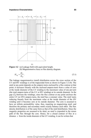


![88 Chapter 3
2
0
1
2 .
n
k
eq
N
X f A T D
H
P S
S ¦ (3.14)
The percentage leakage reactance, with the base impedance as b
Z , is given by
2
0
1
0
1
% 100 100 2 100
( )
2 100
n
k
b eq
n
k
eq
IN
X IX
X f ATD
Z V H V
NI
f ATD
H V N
P S
S
P S
S
u u u
u
¦
¦
(3.15)
where V is the rated voltage and the term N
V is volts/turn of the transformer.
Substituting 7
0 10
4
u
S
P and adjusting the constants so that the dimensions
used in the formula are in units of centimeters ( eq
H in cm and ¦ATD in
cm2
), we obtain
¦
u
n
k
eq
ATD
Turn
Volts
H
Turns
Ampere
f
X
1
5 )
(
10
48
.
2
% . (3.16)
After having derived the general formula, we will now apply it for a simple case
of a two winding transformer shown in Figure 3.2. The constants a and b have
the values of 0 and 1 for the LV winding, 1 and 1 for the gap, and 1 and 0 for the
HV winding, respectively. If g
D
D ,
1 and 2
D are the mean diameters and
1 , ,
g
T T and 2
T are the radial depths of the LV winding, the gap and the HV
winding, respectively, using Equation 3.12 we have
2
2
1
1
3
1
3
1
D
T
D
T
D
T
ATD g
g u
u
u
¦ . (3.17)
The value of eq
H is calculated by Equation 3.1, for which the Rogowski factor
R
K is given by
)
2
1
(
)
2
1
(
1
1
T
g
T
T
w
H
T
g
T
T
w
H
e
KR
S
S
. (3.18)
For taking into account the effect of the core, a more accurate but complex
expression for R
K can be used as given in [1]. For most cases, Equation 3.18
gives sufficiently accurate results.
For autotransformers, transformed ampere-turns should be used in
Equation 3.16 (the difference between the turns corresponding to the phase
voltages of the HV and LV windings multiplied by the HV winding current) and
the calculated impedance is multiplied by the autofactor,
www.EngineeringBooksPDF.com](https://image.slidesharecdn.com/transformer-engineering-design-technology-and-diagnostics-second-edition-pdf-230506172819-680afe24/85/transformer-engineering-design-technology-and-diagnostics-second-edition-pdf-pdf-109-320.jpg)


![Impedance Characteristics 93
where A is the magnetic vector potential and J is the current density vector.
Equation 3.34 can be derived [2] from Equation 3.24,
³
³ ˜
˜
vol
vol
m
dv
I
dv
I
I
W
L J
A
H
B 2
2
2
1
1
2
. (3.35)
The leakage reactance between two windings in a transformer can also be
calculated as
12
2
1
12 2M
X
X
X
(3.36)
where X1 and X2 are the self reactances of the windings and M12 is the mutual
reactance between them. It is difficult to calculate the self and mutual reactances
which depend on saturation effects. Also, since the values of (X1 + X2) and 2M12
are nearly equal and are much higher than the leakage reactance X12, a small
error in the calculation of them results in a large error in the estimation of X12.
Hence, it is always easier to calculate the leakage reactance of a transformer
directly instead of using the formulae in terms of the self and mutual reactances.
Therefore, for finding the effective leakage reactance of a system of windings,
the total power of the system is expressed in terms of the leakage impedances
instead of the self and mutual impedances. Consider a system of windings 1, 2,
…, n, with the leakage impedances jk
Z between the pairs of the windings j and
k. For a negligible magnetizing current (as compared to the rated currents in the
windings) the total power can be expressed as [3]
*
1 1
1 ˆ ˆ ˆ
2
n n
jk j k
k j
P jQ Z I I
¦¦ (3.37)
where *
ˆ
k
I is the complex conjugate of ˆ
k
I . Winding resistances can be neglected
in comparison with much larger leakage reactances. When the current vectors of
the windings are parallel (in phase or phase-opposition), the expression for Q
(which is given by the imaginary part of the previous equation) becomes
*
1 1 1 1
1 1
ˆ ˆ ˆ
Im
2 2
n n n n
jk j k jk j k
k j k j
Q Z I I X I I
ª º
« »
¬ ¼
¦¦ ¦¦ . (3.38)
Equation 3.38 gives the total reactive volt-amperes consumed by all the leakage
reactances of the system of the windings. The effective or equivalent leakage
reactance of the system of n windings, referred to the source (primary) winding
carrying the current Ip , is given by
2
p
eff
I
Q
X in :. (3.39)
www.EngineeringBooksPDF.com](https://image.slidesharecdn.com/transformer-engineering-design-technology-and-diagnostics-second-edition-pdf-230506172819-680afe24/85/transformer-engineering-design-technology-and-diagnostics-second-edition-pdf-pdf-114-320.jpg)
![94 Chapter 3
Figure 3.6 Method of images.
If the currents and jk
X are expressed in per-unit in Equation 3.38, the value of Q
(calculated when the rated current flows in the primary winding) gives directly the
per-unit reactance of the transformer consisting of n windings. The use of this
reactive KVA approach is illustrated in Sections 3.6 and 3.7.
3.3 Analytical Methods
The classical method described in Section 3.1 has certain limitations. The effect
of the core is neglected and it is tedious to take into account axial gaps in
windings and asymmetries in distributions of ampere-turns. Some of the more
commonly used analytical methods, which overcome these difficulties, are now
described. The leakage reactance calculation by more accurate numerical
methods (e.g., FEM) is described in Section 3.4.
3.3.1 Method of images
When computers were not available, many attempts were made to devise
accurate methods of calculating axial and radial components of the leakage field,
and subsequently the leakage reactance. A popular approach was to use simple
Biot-Savart’s law with the effect of the iron core taken into account by the
method of images. The method basically works in the Cartesian (x-y) coordinate
system in which windings are represented by straight coils (assumed to be of
infinite dimensions along the z-axis perpendicular to the plane of the paper)
placed at appropriate distances from a plane surface bounding a semi-infinite
mass of infinite permeability. The effect of the iron core is represented by the
images of the coils as far behind the surface as they are in the front. Parallel
planes have to be added as shown in Figure 3.6 to obtain accurate results, which
leads to an arrangement of infinite images in all the four directions [4]. All these
www.EngineeringBooksPDF.com](https://image.slidesharecdn.com/transformer-engineering-design-technology-and-diagnostics-second-edition-pdf-230506172819-680afe24/85/transformer-engineering-design-technology-and-diagnostics-second-edition-pdf-pdf-115-320.jpg)
![Impedance Characteristics 95
coils should give the same value of the leakage field at any point as that with the
original geometry of the two windings enclosed by the iron boundary. New
planes (mirrors) can be added, one at a time, until the difference between the
successive solutions is negligible; usually the first three or four images are
sufficient. Biot-Savart’s law is then applied to this arrangement of the current
distributions, which is devoid of the magnetic mass (iron), to find the value of
the leakage field at any point.
3.3.2 Roth’s method
A method based on double Fourier series, originally proposed by Roth, was
extended in [5] to calculate the leakage reactance for an irregular arrangement of
windings. The advantage of this method is that it is applicable to uniform as well
as nonuniform distributions of ampere-turns of windings. The arrangement of
windings in the core window can be entirely arbitrary but it should be divisible
into rectangular blocks, each block having a uniform current density distribution
within itself.
In this method, the core window is considered as S radians wide and S
radians long, regardless of its absolute dimensions. The ampere-turn density
distribution as well as the flux distribution is conceived to be consisting of
components which vary harmonically along both the x and y axes. The method
uses a principle similar to that of the method of images; for every harmonic the
maximum value occurs at fictitious planes about which mirroring is done to
simulate the effect of the iron boundary. Reactive volt-amperes ( X
I 2
) are
calculated in terms of these current harmonics for a depth of unit dimension in
the z direction. The total volt-amperes are obtained by multiplying the calculated
values by corresponding mean perimeters. The per-unit value of the leakage
reactance is calculated by dividing X
I 2
by the base volt-amperes. For a
reasonable accuracy, the number of space harmonics in the double Fourier series
should be at least equal to 20 when the ampere-turns are symmetrically
distributed in the LV and HV windings [6]. The accuracy is better with a higher
number of space harmonics. Figure 3.7 shows plots of the radial flux density
along the height of a transformer winding. As the number of the space
harmonics is increased, the variation of the flux density becomes smooth
indicating a better accuracy.
3.3.3 Rabin’s method
If the effect of curvatures of the windings needs to be taken into account in
Roth’s formulation, the method becomes complicated, and in that case Rabin’s
method is more suitable [4, 7]. It solves the following Poisson’s equation in
cylindrical coordinates,
2
’ A = P
J (3.40)
www.EngineeringBooksPDF.com](https://image.slidesharecdn.com/transformer-engineering-design-technology-and-diagnostics-second-edition-pdf-230506172819-680afe24/85/transformer-engineering-design-technology-and-diagnostics-second-edition-pdf-pdf-116-320.jpg)
![96 Chapter 3
Figure 3.7 The effect of the number of space harmonics on the accuracy.
where A is the magnetic vector potential and J is the current density having only
the angular component. Therefore, in cylindrical coordinates the equation
becomes
T
T
T
T
T
P J
z
A
r
A
r
A
r
1
r
A
2
2
2
2
2
w
w
w
w
w
w
. (3.41)
In this method, the current density is assumed to depend only on the axial
position and hence can be represented by a single Fourier series with
coefficients which are Bessel and Struve functions. For a reasonable accuracy,
the number of space harmonics should be about 70 [6].
3.4 Numerical Method for Reactance Calculation
The finite element method (FEM) is the most commonly used numerical method
for the reactance calculation of nonstandard configurations of windings and
asymmetrical/nonuniform distributions of ampere-turns, which cannot be easily
and accurately handled by the classical method given in Section 3.1. The FEM
analysis can be more accurate than the analytical methods described in Section
3.3. User-friendly commercial FEM software packages are now available. A 2-D
FEM analysis can be integrated into routine design calculations. The main
www.EngineeringBooksPDF.com](https://image.slidesharecdn.com/transformer-engineering-design-technology-and-diagnostics-second-edition-pdf-230506172819-680afe24/85/transformer-engineering-design-technology-and-diagnostics-second-edition-pdf-pdf-117-320.jpg)
![Impedance Characteristics 97
advantage of FEM is that any complex geometry can be analyzed since its
formulation depends only on the class of problem and is independent of
geometrical details. It can also take into account material discontinuities easily.
The theory of the FEM technique and its applications to transformers are
elaborated in Chapter 12. Here, the technique is briefly illustrated when applied
to calculate the leakage reactance of a transformer.
The problem geometry is divided into small elements [8, 9]. Within each
element, the flux density is assumed constant so that the magnetic vector
potential varies linearly within each element (a first order approximation); in
Cartesian coordinates the potential can be approximated as
y
c
x
b
a
A
. (3.42)
For a better accuracy, the potential can be assumed to vary as a polynomial of a
degree higher than one. The elements are generally of triangular or tetrahedral
shape. The windings are modeled as rectangular blocks; if the distribution of
ampere-turns is not uniform, they are divided into suitable sections so that the
current density in each section is uniform. A typical configuration of the LV and
HV windings in a transformer is shown in Figure 3.8. The main steps involved
in the analysis are now outlined.
1. Creation of geometry: The geometry shown in Figure 3.8 is simple. In case of
complex 2-D or 3-D geometries, many commercial FEM programs allow the
import of figures drawn in drafting packages, which makes it easier and less
time consuming to create geometries. The problem domain has to be always
bounded by a boundary (e.g., abcda in Figure 3.8). 2-D problems can be solved
either in Cartesian or cylindrical coordinates. Since transformers are 3-D
structures, both the systems lead to approximations and corresponding errors.
L
V
H
V
yoke
yoke
limb limb
a
e
d
h
f g
b c
Figure 3.8 Geometry for FEM analysis.
www.EngineeringBooksPDF.com](https://image.slidesharecdn.com/transformer-engineering-design-technology-and-diagnostics-second-edition-pdf-230506172819-680afe24/85/transformer-engineering-design-technology-and-diagnostics-second-edition-pdf-pdf-118-320.jpg)


![Impedance Characteristics 101
100
70 50
23
LV
HV
HV
1260
I
560 LV
433
turns
1000
turns
HV1
1.0 1.0 HV2
50
turns
50
turns
0.05
100
turns
567
567
TAP 126
Figure 3.10 Details of the transformer in Example 3.1.
The leakage reactance can be calculated from Equation 3.16 as
%
64
.
14
1
.
871
21
.
76
4
.
133
)
1000
78
.
137
(
50
10
48
.
2 5
LV_HV1 u
u
u
u
u
u
X .
The winding HV2 is made up of two sections. The AT diagram for the top
section is shown in Figure 3.10. The section has two windings, each having
ampere-turns of 0.05 per-unit [= )
78
.
137
1000
(
)
78
.
137
50
( u
u ]. For this section,
cm
0
.
10
,
cm
3
.
6
,
cm
0
.
0
,
cm
7
.
56 2
1 w
g H
T
T
T .
It is to be noted here that the winding height for the calculation is the dimension
in the radial direction, which is equal to 10.0 cm. Equations 3.18 and 3.1 give
213
0.
KR and cm
0
.
47
213
.
0
10
R
w
eq K
H
H .
The term ATD is calculated for each part using Equation 3.12, the
corresponding values of a and ,
b and the mean diameter of the HV winding,
0
5
6
94
05
0
3
3
6
6
94
05
0
0
0
6
94
05
0
3
7
56 2
2
2
.
.
.
.
.
.
.
.
.
.
ATD u
u
u
u
u
u
¦ .
The leakage reactance of the section can be calculated from Equation 3.16 as
%
24
.
0
0
.
5
21
.
76
0
.
47
)
1000
78
.
137
(
50
10
48
.
2 5
u
u
u
u
u
u
S
X .
The HV2 winding comprises of two such sections connected in series. Hence,
the total reactance contributed by the HV2 winding is two times the reactance of
a single section as explained in Section 3.1.2.
%
48
.
0
24
.
0
2
HV2 u
? X .
www.EngineeringBooksPDF.com](https://image.slidesharecdn.com/transformer-engineering-design-technology-and-diagnostics-second-edition-pdf-230506172819-680afe24/85/transformer-engineering-design-technology-and-diagnostics-second-edition-pdf-pdf-122-320.jpg)


![Impedance Characteristics 105
1
2
3
R2 X
R3 X3
R1 X1
2
1
2
3
Three-winding transformer Star equivalent circuit
Figure 3.12 Representation of a three-winding transformer.
It follows from the above three equations that the individual reactances in the
star equivalent circuit are given by
@
23
13
12
1
2
1
X
X
X
X
(3.47)
@
13
23
12
2
2
1
X
X
X
X
(3.48)
@
12
23
13
3
2
1
X
X
X
X
. (3.49)
A rigorous derivation of the above three equations and the evolution of the star
equivalent circuit is given in [10].
Similarly, the percentage resistances can be derived as
@
23
13
12
1
2
1
R
R
R
R
(3.50)
@
13
23
12
2
2
1
R
R
R
R
(3.51)
@
12
23
13
3
2
1
R
R
R
R
. (3.52)
Note that these percentage resistances represent the total load loss (the addition
of the DC-resistance R
I 2
loss in windings, the eddy loss in windings and the
stray loss in structural parts).
www.EngineeringBooksPDF.com](https://image.slidesharecdn.com/transformer-engineering-design-technology-and-diagnostics-second-edition-pdf-230506172819-680afe24/85/transformer-engineering-design-technology-and-diagnostics-second-edition-pdf-pdf-126-320.jpg)
![106 Chapter 3
R2 X2
3
R X3
3
1
2 R1 X1
V3
1
2
3
Figure 3.13 Mutual effect in star equivalent network.
The leakage reactances in the star equivalent network are basically the
mutual load reactances between different circuits. For example, the reactance
1
X in Figure 3.12 is the common or mutual reactance to the loads in circuits 2
and 3. A current flowing from circuit 1 to either circuit 2 or 3 produces voltage
drops across 1
R and 1
X , and hence affects the voltages in circuits 2 and 3.
When a voltage is applied to winding 1 with winding 2 short-circuited as shown
in Figure 3.13, the voltage across the open-circuited winding 3 is equal to the
voltage drop across the leakage impedance, 2
Z , of circuit 2.
The individual leakage reactance of a winding can be negative. The total
leakage reactance between a pair of windings cannot be negative but the mutual
effect between two circuits may be negative when a load current flows [11].
Negative impedances are virtual values, and they reproduce faithfully the
terminal characteristics of transformers. The three windings are interlinked, and
hence a load current flowing in a winding affects the voltages in the other two
windings, sometimes in a surprising way. For example, a lagging load on a
winding may increase the voltage magnitude of another winding due to the
presence of a negative value of a leakage reactance (capacitive reactance) in the
equivalent circuit.
Similarly, a negative resistance may appear in the star equivalent network
of an autotransformer with a tertiary winding or of a high efficiency transformer
whose stray loss is much higher as compared to the ohmic losses in its windings
(e.g., when a lower value of the current density is used for the windings).
In Chapter 1, we have seen how the regulation of a two-winding
transformer is calculated. The calculation of the voltage regulation of a three-
winding transformer is explained with the help of the following example.
Example 3.3
Find the voltage drop between the terminals of a three-winding transformer,
when the load on the IV winding is 70 MVA at 0.8 lagging power factor, and the
load on the LV winding is 30 MVA at 0.6 lagging power factor. The transformer
data is:
www.EngineeringBooksPDF.com](https://image.slidesharecdn.com/transformer-engineering-design-technology-and-diagnostics-second-edition-pdf-230506172819-680afe24/85/transformer-engineering-design-technology-and-diagnostics-second-edition-pdf-pdf-127-320.jpg)

![108 Chapter 3
The effective power factor ( 1
cosT ) and the effective load taken as a fraction
( 1
K ) of the base MVA for the primary (220 kV) circuit are determined by
solving the following two equations:
74
.
0
6
.
0
3
.
0
8
.
0
7
.
0
cos
cos
cos 3
3
2
2
1
1 u
u
T
T
T K
K
K (3.53)
66
.
0
8
.
0
3
.
0
6
.
0
7
.
0
sin
sin
sin 3
3
2
2
1
1 u
u
T
T
T K
K
K (3.54)
Solving these two equations we obtain
67
.
0
sin
,
75
.
0
cos
,
99
.
0 1
1
1 T
T
K .
Therefore, the primary circuit voltage drop (regulation) is
%
23
.
10
67
.
0
25
.
15
75
.
0
1625
.
0
99
.
0
)
sin
cos
( 1
1
1
1
1
1 u
u
T
T
H X
R
K .
Now, the voltage drops between the terminals can be calculated as
%
2
.
10
)
03
.
0
(
23
.
10
2
1
2
1
H
H
H
%
84
.
12
61
.
2
23
.
10
3
1
3
1
H
H
H
%
64
.
2
61
.
2
03
.
0
3
2
3
2
H
H
H .
While calculating 3
2
H , a minus sign is used for 2
H as the drop in the voltage is
in the direction opposite to the direction of the corresponding current flow.
When there are more than three windings, transformers cannot be in
general represented by a pure star or mesh equivalent circuit. The equivalent
circuit should have 2
/
)
1
(
n
n independent impedance links, where n is the
number of windings. A four-winding transformer has six independent links with
four terminal points. The procedure for determining the values of impedances in
the equivalent circuit of a transformer having four or more windings is given in
[1, 12, 13].
zig
zag
N a b c
Figure 3.15 A zigzag connection.
www.EngineeringBooksPDF.com](https://image.slidesharecdn.com/transformer-engineering-design-technology-and-diagnostics-second-edition-pdf-230506172819-680afe24/85/transformer-engineering-design-technology-and-diagnostics-second-edition-pdf-pdf-129-320.jpg)
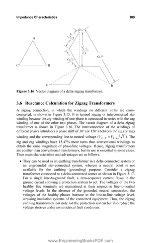
![110 Chapter 3
N
3
A
B
C
fault
I I0
0
I0
I
I I0
0
I0
0
Figure 3.17 A zigzag earthing transformer.
x Zigzag transformers offer a specific advantage when used in applications
consisting of power electronic converters. The DC magnetization due to
asymmetry in firing angles is cancelled in each limb due to opposite
directions of the DC currents flowing in its zig and zag windings. Similarly,
the DC magnetization inherent in a three-pulse mid point rectifier
connection is eliminated if the secondary winding is of zigzag type [14].
x Earthing transformers offer a low impedance path to zero-sequence currents
under asymmetrical fault conditions because the only magnetic flux
produced by the currents is the leakage flux; the magnetizing flux in each
limb is zero due to the equal and opposite currents flowing in its zig and zag
windings as shown in Figure 3.17. Owing to a very low impedance of the
earthing transformer, it may be necessary to limit currents under fault
conditions by connecting a resistor between the neutral and the earth. Under
normal operating conditions, only a small exciting current flows in the
windings of the earthing transformer.
x Third harmonic voltage components present in the zig and zag windings are
cancelled in the lines.
The reactance of a transformer consisting of zigzag and star (or delta)
windings can be calculated from reactive volt-amperes. Consider the star-zigzag
transformer shown in Figure 3.18. The currents b
a I
I , and c
I are assumed to
flow from the line terminals to the neutral for convenience. The corresponding
vector diagram is also shown in the figure.
www.EngineeringBooksPDF.com](https://image.slidesharecdn.com/transformer-engineering-design-technology-and-diagnostics-second-edition-pdf-230506172819-680afe24/85/transformer-engineering-design-technology-and-diagnostics-second-edition-pdf-pdf-131-320.jpg)
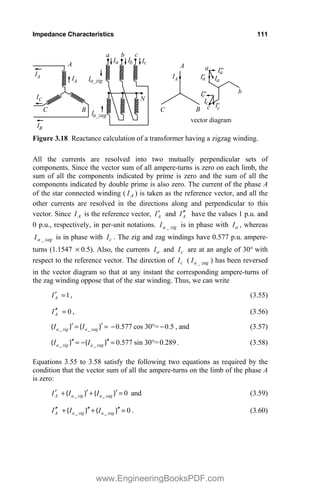


![Impedance Characteristics 117
3.7.1 Open-circuit zero-sequence reactance without delta winding
A. Three-phase three-limb transformers
For a three-phase three-limb transformer, since the zero-sequence fluxes in the
three limbs are in the same direction, they have to return through a path outside
the core. In this case, the tank acts as an equivalent delta winding, and the open-
circuit zero-sequence reactance is the one between the tank and the excited
winding. Since the gap/area between the excited winding and the tank is much
higher than the gap/area between the LV and HV windings, the open-circuit
zero-sequence reactance is considerably higher than the short-circuit positive-
sequence reactance (the usual leakage impedance between the windings),
although it is much lower than the open-circuit positive sequence reactance
obtained by the standard open-circuit test discussed in Chapter 1. The tank
influences the zero-sequence reactance in the following way. It provides a lower
reluctance return path (as compared to air) to the zero-sequence flux, which has
the effect of increasing the reactance; on the other hand the tank enclosing the
three phases acts as a short-circuited winding reducing the reactance. The latter
effect is more dominant and hence the zero-sequence reactance inside the tank is
appreciably less than that without it [15]. However, the zero-sequence reactance
is much larger than the positive-sequence impedance as mentioned earlier.
The reactance between the excited winding and the tank can be calculated
by the procedure given in Section 3.1.1 with the latter represented as an
equivalent (fictitious) winding with zero radial depth (contribution of the tank to
the AT diagram area can be neglected due to its small thickness). The winding-
tank gap can be taken as the equivalent distance which gives approximately the
same area of the space between them. The zero-sequence reactance is then
calculated by using Equation 3.16 as
)
3
1
(
)
(
10
48
.
2
% 5
0 g
g
w
w
eq
D
T
D
T
Turn
Volts
H
Turns
Ampere
f
X u
u
u
u
u
u
u
(3.66)
where
w
T radial depth of the excited winding in cm
w
D mean diameter of the excited winding in cm
g
T gap between the excited winding and the tank in cm
g
D mean diameter of the gap between the excited winding and the tank
in cm.
When sufficient voltage is applied during the test, the zero-sequence flux
passing through the tank usually saturates it. If the test is done at a voltage
magnitude which does not saturate the tank made generally from mild steel
material, its higher permeability will increase the reactance. Hence, the
reactance calculated using Equation 3.66 has to be suitably corrected by an
www.EngineeringBooksPDF.com](https://image.slidesharecdn.com/transformer-engineering-design-technology-and-diagnostics-second-edition-pdf-230506172819-680afe24/85/transformer-engineering-design-technology-and-diagnostics-second-edition-pdf-pdf-138-320.jpg)
![118 Chapter 3
empirical factor which can be derived based on a set of measurements at various
voltage levels. The correction factor depends on the applied voltage as shown in
Figure 3.22 [16]. The curve in the figure has the same nature as that of the
permeability versus magnetic field intensity graph derived from the
measurements on a typical grade of mild steel material (Figure 3.23) [17].
B. Three-phase five-limb and single-phase three-limb transformers
In a three-phase five-limb transformer, the zero-sequence flux has a return path
through the end yokes and the end limbs, and hence the open-circuit zero-
sequence reactance equals the open-circuit positive-sequence reactance (a high
value) unless the voltage applied is such that the yokes and the end limbs
saturate. For an applied zero-sequence voltage close to the rated value of the
excited winding, the yokes and the end limbs will be completely saturated; their
area is too less to carry the zero-sequence flux of all the three phases at the rated
voltage. This results in a lower value of the open-circuit zero-sequence
reactance, which can be close to that for the three-phase three-limb construction.
0 25
% Zero sequence voltage
1.0
Correction
factor
50 75
1.5
Figure 3.22 Correction factor for the zero-sequence reactance [16].
0 1000 2000 3000 4000
200
400
600
800
1000
1200
Magnetic field intensity in A/m
Relative
permeability
Figure 3.23 Variation of r
P with field intensity in mild steel material [17].
www.EngineeringBooksPDF.com](https://image.slidesharecdn.com/transformer-engineering-design-technology-and-diagnostics-second-edition-pdf-230506172819-680afe24/85/transformer-engineering-design-technology-and-diagnostics-second-edition-pdf-pdf-139-320.jpg)
![Impedance Characteristics 119
For single-phase three-limb transformers, since the zero-sequence flux
returns through the end limbs, the open-circuit zero-sequence reactance is equal
to the open-circuit positive-sequence reactance (~ infinite value). Thus, for a
bank of three single-phase transformers, the zero-sequence characteristics are
usually identical to the positive-sequence characteristics [18].
3.7.2 Open-circuit zero-sequence reactance with a delta-connected winding
With one delta connected secondary winding, a zero-sequence current circulates
in the closed delta. Thus, the transformer acts as if it is short-circuited regardless
of whether the winding is loaded or not. Let us again consider the following two
cases.
A. Three-phase three-limb transformers
When zero-sequence voltage is applied to the star-connected winding, zero-
sequence currents flow in the delta-connected winding and the tank which acts
as an equivalent short-circuited (delta) winding. In order to estimate the current
division between these two windings and the zero-sequence reactance, we will
use the method described in Section 3.2 for a composite system of windings. Let
the star-connected primary winding, the delta connected secondary winding and
the tank be represented by notations 1, 2, and 3 respectively. Applying Equation
3.38, for the present case of the three windings (one star- and two delta-
connected windings), we obtain the per-unit value of zero-sequence reactance as
@
)
(
2
)
)(
(
2
)
(
2
2
1
3
1
13
3
2
23
2
1
12
0 I
I
X
I
I
X
I
I
X
X
Q
. (3.67)
The currents in windings 2 and 3 are assigned a negative sign as their direction
is opposite to that of the current in the primary winding. Since the magnetizing
current can be neglected,
3
2
1 I
I
I . (3.68)
If the magnitude of the applied zero-sequence voltage is such that the rated
current flows in the primary winding (i.e., 1
I has a value of 1 per-unit), then
2
3 1 I
I . (3.69)
)
1
(
)
1
( 2
13
2
2
23
2
12 I
X
I
I
X
I
X
Q
? . (3.70)
The currents are distributed in the windings in such a way that the total energy is
minimized. Hence, differentiating Q with respect to 2
I and equating the
derivative to zero, we have
www.EngineeringBooksPDF.com](https://image.slidesharecdn.com/transformer-engineering-design-technology-and-diagnostics-second-edition-pdf-230506172819-680afe24/85/transformer-engineering-design-technology-and-diagnostics-second-edition-pdf-pdf-140-320.jpg)


![122 Chapter 3
LV
I
390
470
300
360
I
I
I 30
HV
40
15
600
Figure 3.24 Dimensions of 2 MVA transformer.
955
.
0
1
1
)
0
.
4
5
.
1
0
.
3
(
0
.
60
)
0
.
4
5
.
1
0
.
3
(
0
.
60
S
S
e
KR .
The equivalent winding height according to Equation 3.1 is
8
62
955
0
60 .
.
/
K
/
H
H R
w
eq .
¦ATD is calculated using Equation 3.17,
6
146
0
43
0
4
3
1
5
37
5
1
0
33
0
3
3
1
.
.
.
.
.
.
.
ATD u
u
u
u
u
¦ .
For calculating the reactance, either the LV or HV ampere-turns are used (their
values are equal since the magnetizing ampere-turns are neglected).
LV current = 67
2666
433
3
10
2 6
.
u
u
A and LV turns = 16
625
15
3
433
.
.
The positive-sequence leakage reactance is given by Equation 3.16,
%
9
.
7
6
.
146
625
.
15
8
.
62
)
16
67
.
2666
(
50
10
48
.
2
% 5
u
u
u
u
u
u
p
X .
Since the delta-connected HV winding is the outer winding, the zero-sequence
reactance of the star-connected winding is approximately equal to the positive-
sequence leakage reactance as explained in Section 3.7.2. However, during the
actual test, one usually gets the value of zero-sequence reactance higher than the
positive-sequence leakage reactance by an amount corresponding to the voltage
drop in the neutral bar. The reactance of a neutral bar having rectangular
dimensions ( b
a u ) is given by the expression [19, 20]:
www.EngineeringBooksPDF.com](https://image.slidesharecdn.com/transformer-engineering-design-technology-and-diagnostics-second-edition-pdf-230506172819-680afe24/85/transformer-engineering-design-technology-and-diagnostics-second-edition-pdf-pdf-143-320.jpg)


![Impedance Characteristics 125
Similarly,
5
2 _
2.48 10 50 137.78 908 1
( ) 10 94.6 25 129.6
137.2 83.93 3
47.89% .
z oc
X
u u u u § ·
u u u u
¨ ¸
u © ¹
The zero-sequence reactance as seen from the inner LV winding with the outer
HV winding short-circuited is the same as the positive-sequence leakage
reactance (if the reactance contributed by the neutral bar is neglected),
%
16
.
12
)
( _
12 p
sc
z X
X .
The zero-sequence reactance as seen from the HV winding with the LV winding
short-circuited is calculated using Equation 3.79,
%
44
.
9
73
.
61
89
.
47
16
.
12
)
(
)
(
)
(
_
1
_
2
_
21 u
u
oc
z
oc
z
p
sc
z
X
X
X
X .
The zero-sequence network [18] of this two winding transformer is shown in
Figure 3.26 which satisfies all the calculated zero-sequence reactance values,
,
)
( _
1 oc
z
X oc
z
X _
2
)
( , sc
z
X _
12
)
( and sc
z
X _
21
)
( .
For example, the zero-sequence reactance as seen from the (excited) HV
winding with the short-circuited LV winding is
%
43
.
9
73
.
48
0
.
13
73
.
48
0
.
13
835
.
0
)
73
.
48
//
0
.
13
(
835
.
0
)
( _
21
u
sc
z
X ,
which matches closely with the value calculated previously.
In a similar way, the zero-sequence reactance of a three-winding three-
phase three-limb transformer can be estimated as demonstrated by the following
example.
LV HV
-0.835%
13%
48.73%
Figure 3.26 The zero-sequence network of the two-winding transformer in
Example 3.6.
www.EngineeringBooksPDF.com](https://image.slidesharecdn.com/transformer-engineering-design-technology-and-diagnostics-second-edition-pdf-230506172819-680afe24/85/transformer-engineering-design-technology-and-diagnostics-second-edition-pdf-pdf-146-320.jpg)


![128 Chapter 3
Here, the system of four windings (i.e., the tertiary, LV and HV windings plus
an imaginary winding representing the currents flowing in the tank) is converted
into the equivalent three-winding system which takes into account the effect of
the tank while calculating the short-circuit zero-sequence reactance between any
two of the tertiary, LV and HV windings. Hence, the calculation of 21
3 _
z
X by
the star equivalent circuit of Figure 3.28 is an approximate way. Actually, the
problem needs to be solved with an additional delta-connected winding
representing the tank.
Let us now calculate the reactance by treating the tank as the fourth wind-
ing. The zero-sequence reactance can be calculated by the procedure given in Sec-
tion 3.2 (i.e., the reactive kVA approach). Let 1
I , 2
I and 4
I be the currents flow-
ing through the tertiary, LV and equivalent delta (tank) windings respectively. The
current flowing through the HV winding ( 3
I ) is 1 per-unit and we know that
4
2
1
3 1 I
I
I
I
.
The expression for Q is
¸
¸
¹
·
¨
¨
©
§
4
3
34
4
2
24
3
2
23
4
1
14
3
1
13
2
1
12
2
2
2
2
2
2
2
1
I
I
X
I
I
X
I
I
X
I
I
X
I
I
X
I
I
X
Q
p
p
p
p
p
p
.
The reactance between the tank and any other winding has already been calculated
(e.g., %
81
.
64
)
(
)
( _
1
14 oc
z
p X
X ). By putting the values of all the reactances
and using 4
2
1 1 I
I
I
, the above expression becomes
2
4
2
2
4
2
4
2 81
64
6
1
13
52
46
04
14
64
22 I
.
I
I
I
.
I
.
I
.
.
Q
.
In order to have a minimum energy state, we differentiate the above expression
with respect to 2
I and 4
I , and equate the derivatives to zero and obtain two si-
multaneous equations. These two equations are solved to give
8747
0
2 .
I and 2705
0
4 .
I .
Putting these values in the expression for Q, we have %
21
.
10
)
( 21
_
3
z
X , which
is close to that calculated by using the star equivalent circuit (i.e., 10.27%).
The methods described for the calculation of zero-sequence reactances can
give reasonably accurate results and should be refined by empirical correction
factors, if required, based on the results of tests conducted on a number of
transformers. For more accurate calculations, numerical methods like FEM can
be used [21, 22], in which the effect of the tank saturation on the zero-sequence
reactance can be exactly simulated. The tank material should be modeled by
defining its conductivity and nonlinear B-H characteristics. In power
www.EngineeringBooksPDF.com](https://image.slidesharecdn.com/transformer-engineering-design-technology-and-diagnostics-second-edition-pdf-230506172819-680afe24/85/transformer-engineering-design-technology-and-diagnostics-second-edition-pdf-pdf-149-320.jpg)


![Impedance Characteristics 131
The five-limb and the shell form constructions are better-suited for unbalanced
operations, since there is a path for the zero-sequence flux in them.
The magnetic circuit of three-phase five-limb transformers/banks of
single-phase transformers can be visualized as a closed one giving a very high
value of the zero-sequence reactance. If a delta-connected stabilizing winding is
added to these three types of transformers, three-phase three-limb transformers,
banks of three single-phase three-limb transformers, and three-phase five-limb
transformers, the difference between the zero-sequence reactance characteristics
of the three-phase three-limb transformers and that of the other two types
diminishes. As long as one delta-connected winding is present, it makes a very
little difference whether it is an effectively open or closed magnetic circuit from
the zero-sequence reactance point of view.
A frequently asked question is whether the stabilizing winding can be
dispensed with in the three-phase three-limb star-star (or auto-star) connected
transformers with the grounded neutral condition. This is because, as seen in the
previous section, the high reluctance nonmagnetic path offered to the zero-
sequence flux results in a lower zero-sequence reactance as compared to the
positive-sequence reactance, and thus to some extent the effect of the stabilizing
winding is achieved. Whether or not the stabilizing winding can be omitted
depends mainly on whether the zero-sequence and third harmonic characteristics
are compatible with the system into which the transformer is going to be
installed. If these two characteristics are not adversely affected in the absence of
the stabilizing winding, it may be omitted [23]. Away from distribution points,
in transmission networks the loading of the three phases of transformers is more
or less balanced. Also, if the telephone-interference problem due to harmonic
currents is within limits, and if the zero-sequence currents during asymmetrical
fault conditions are large enough to be easily detected, the provision of the
stabilizing winding in the three-phase three-limb transformers can be reviewed.
This is because, since the stabilizing winding is generally unloaded, its
conductor dimensions tend to be smaller. Such a winding becomes weak and
vulnerable under asymmetrical fault conditions, which is a subject of discussion
in Chapter 6.
Consequences of omitting the stabilizing winding in banks of three single-
phase transformers/three-phase five-limb transformers can be significant. The
zero-sequence reactance will be higher, and if the disadvantages of its high
value cannot be tolerated, the stabilizing winding cannot be omitted. A low
voltage stabilizing winding, with its terminal brought out, helps in very large
transformers for carrying out tests such as the no-load loss test in the
manufacturer’s works. In the absence of this winding, it may not be possible to
do the test if the manufacturer does not have a high-voltage source or a suitable
step-up transformer. Alternatively, a star-connected auxiliary winding can be
provided for the testing purpose, whose terminals can be buried inside the tank
after the testing.
www.EngineeringBooksPDF.com](https://image.slidesharecdn.com/transformer-engineering-design-technology-and-diagnostics-second-edition-pdf-230506172819-680afe24/85/transformer-engineering-design-technology-and-diagnostics-second-edition-pdf-pdf-152-320.jpg)


![Eddy Currents and Winding Stray Losses 141
4.2 Poynting Vector
Poynting’s theorem is the expression of the law of conservation of energy applied
to electromagnetic fields. When the displacement current is neglected, as in the
previous section, Poynting’s theorem can be mathematically expressed as [1, 2]
v
v
t
s
v
v
s
d
d
d
)
( ³
³
³ ˜
w
w
˜
˜
u
E
J
B
H
n
H
E (4.40)
where v is the volume enclosed by the surface s and n is the unit vector normal to
the surface directed outwards. Using Equation 4.5, the above equation can be
modified as
v
v
t
s
v
v
s
d
1
d
d
)
( ³
³
³
w
w
˜
˜
u
2
J
B
H
n
H
E
V
. (4.41)
This is a simpler form of Poynting’s theorem which states that the net inflow of
power is equal to the sum of the power absorbed by the magnetic field and the
ohmic loss. The Poynting vector is given by the vector product,
E
P H
u (4.42)
which expresses the instantaneous density of power flow at a point.
Now, with E having only an x component which varies as a function of z
only, Equation 4.17 becomes
y
x
H
j
z
E
ZP
w
w
, 0
x
H , 0
z
H . (4.43)
Substituting the value of Ex from Equation 4.34 and rearranging we obtain
ZP
J
ZP
J
j
E
e
E
z
j
H x
z
xp
y
w
w
u
)
(
1
(4.44)
The ratio of x
E to y
H is defined as the intrinsic impedance,
J
ZP
K
j
H
E
y
x
. (4.45)
Substituting the value of J from Equation 4.30 we obtain
V
ZP
ZPV
ZP
K
j
j
j
. (4.46)
Using Equation 4.38, the above equation can be rewritten as
www.EngineeringBooksPDF.com](https://image.slidesharecdn.com/transformer-engineering-design-technology-and-diagnostics-second-edition-pdf-230506172819-680afe24/85/transformer-engineering-design-technology-and-diagnostics-second-edition-pdf-pdf-162-320.jpg)
![142 Chapter 4
G
V
G
V
V
V
G
K
q
‘
u
q
‘
»
»
¼
º
«
«
¬
ª 45
2
2
90
1
1
2
1
j . (4.47)
Now, Equation 4.36 can be rewritten in terms of the skin depth as
)
cos( G
Z
G
z
t
e
E
E z
xp
x
. (4.48)
Using Equations 4.45 and 4.47, y
H can be expressed as
)
4
cos(
2
S
G
Z
VG G
z
t
e
E
H z
xp
y . (4.49)
Since E is in the x direction and H is in the y direction, the Poynting vector, which
is a cross product of E and H according to Equation 4.42, is in the z direction.
)
4
cos(
)
cos(
2
2
2 S
G
Z
G
Z
VG G
? z
t
z
t
e
E
H
E
P z
xp
y
x
z (4.50)
Using the identity @
)
cos(
)
cos(
2
1
cos
cos B
A
B
A
B
A
, the above equation
simplifies to
»
¼
º
«
¬
ª
¿
¾
½
¯
®
4
cos
)
4
2
2
cos(
2
1
2
2
2 S
S
G
Z
VG G z
t
e
E
P z
xp
z . (4.51)
The time average Poynting vector is then given by
G
G VG
S
VG z
xp
z
xp
avg
z e
E
e
E
P 2
2
2
2
4
4
cos
2
2
1
)
(
. (4.52)
Thus, it can be observed that at a distance of one skin depth ( G
z ), the power
density is only 0.135 (= 2
e ) times its value at the surface. This is an important
fact for the analysis of eddy currents and losses in structural components of
transformers. If the eddy losses in the tank of a transformer due to the incident
leakage field emanating from windings are being analyzed by using FEM, there
should be at least two or three elements in one skin depth for obtaining accurate
results.
Let us now consider a conductor with a field Exp and the corresponding
current density Jxp at the surface as shown in Figure 4.1. The fields have the value
of 1 p.u. at the surface. The total power loss in the height (i.e., length) h and the
width b is given by the value of power crossing the conductor surface [2] within
the area (h u b),
www.EngineeringBooksPDF.com](https://image.slidesharecdn.com/transformer-engineering-design-technology-and-diagnostics-second-edition-pdf-230506172819-680afe24/85/transformer-engineering-design-technology-and-diagnostics-second-edition-pdf-pdf-163-320.jpg)

![144 Chapter 4
The total ohmic power loss is given by
G
S
Z
V
V
bh
t
J
v
J
P
xp
v
u
¸
¸
¹
·
¨
¨
©
§
¸
¹
·
¨
©
§
³ 4
cos
2
1
d
1 2
2
2
. (4.56)
The average value of power can be expressed as
¸
¸
¹
·
¨
¨
©
§
¿
¾
½
¯
®
¸
¹
·
¨
©
§
¸
¸
¹
·
¨
¨
©
§
¸
¹
·
¨
©
§
4
2
cos
1
2
1
2
4
cos
2
2
2
2 S
Z
V
G
S
Z
V
G
t
avg
J
bh
t
avg
J
bh
P xp
xp
avg .
(4.57)
Since the average value of a cosine term over an integral number of periods is zero
we have
2
4
xp
avg J
bh
P
V
G
(4.58)
which is the same as Equation 4.53. Hence, the average power loss in a conductor
may be computed by assuming that the total current is uniformly distributed in one
skin depth. This is an important result which can be used while calculating eddy
current losses in conductors by numerical methods. When a numerical method
such as FEM is used for estimating stray losses in the tank of a transformer, it is
important to have the element size less than the skin depth of the tank material as
explained earlier. With the overall dimensions of the field domain in meters, it is
difficult to have very small elements inside the tank thickness. Hence, it is
convenient to use analytical results to simplify the numerical analysis. For
example, Equation 4.58 is used in [3] for the estimation of tank losses by 3-D
FEM analysis. The method assumes uniform current density in the skin depth
allowing the use of relatively larger element sizes. The above-mentioned problem
of modeling and analysis of small skin depths can also be handled by using the
concept of surface impedance. The intrinsic impedance can be rewritten from
Equation 4.46 as
V
ZP
V
ZP
V
ZP
V
ZP
K
2
2
45
1 j
j
jX
R
q
‘
. (4.59)
The real part of the impedance, called surface resistance, is given by
V
ZP
2
R . (4.60)
After calculating the r.m.s. value of the tangential component of the magnetic field
intensity (Hrms) at the surface of the tank or any other structural component in the
transformer by either numerical or analytical methods, the specific loss per unit
surface area can be calculated by the following expression [4],
www.EngineeringBooksPDF.com](https://image.slidesharecdn.com/transformer-engineering-design-technology-and-diagnostics-second-edition-pdf-230506172819-680afe24/85/transformer-engineering-design-technology-and-diagnostics-second-edition-pdf-pdf-165-320.jpg)
![Eddy Currents and Winding Stray Losses 145
2
2
2
rms
rms H
H
R
P
V
ZP
. (4.61)
Thus, the total losses in the transformer tank can be determined by integrating the
specific loss over its internal surface.
4.3 Eddy Current and Hysteresis Losses
All the analysis done previously assumed linear material (B-H) characteristics
meaning that the permeability ( P ) is constant. The material used for structural
components in transformers is usually magnetic steel (mild steel), which is a
ferromagnetic material having a much larger value of relative permeability ( r
P )
as compared to that of free space (for which r
P =1). The material has nonlinear B-
H characteristics and the permeability itself is a function of H. Moreover, the
characteristics also exhibit hysteresis. Equation 4.6 ( P
B H ) has to be suitably
modified to reflect the nonlinear characteristics and the hysteresis phenomenon.
The core properties are generally expressed in terms of its permeability and
losses. In an alternative way, the properties can be described by a single quantity
known as complex (or elliptic) permeability. With the help of this type of
representation, it is possible to represent the core by a simple equivalent electric
circuit and the core losses can be expressed as a function of frequency.
If B is assumed to be a sinusoidal quantity, H will be non-sinusoidal due to a
typical shape of the hysteresis loop. In the complex permeability representation,
the harmonics are neglected, and only the fundamental components of B and H
are considered. The magnetic field intensity (H) and the current are in phase,
whereas the flux density (B) and the voltage are in perfect quadrature relationship;
the voltage V leads B or flux by 90 degrees according to Equation 1.1 which in the
time-harmonic form becomes [5]:
ˆ ˆ
B V
j
N Ac
Z
§ ·
¨ ¸
¨ ¸
© ¹
= .
Here, B̂ and ˆ
V are phasors, and Ac is the cross-sectional area having magnetic
path length l with N turns wound around it. In this discussion on complex
permeability, caps are put on phasor quantities. We also know that
ˆ ˆ
N
H I
l
§ ·
¨ ¸
© ¹
ˆ
ˆ
ˆ
ˆ 2
B jl
Z
H N Ac
P
Z
§ ·
¨ ¸
?
¨ ¸
¨ ¸
© ¹
.
www.EngineeringBooksPDF.com](https://image.slidesharecdn.com/transformer-engineering-design-technology-and-diagnostics-second-edition-pdf-230506172819-680afe24/85/transformer-engineering-design-technology-and-diagnostics-second-edition-pdf-pdf-166-320.jpg)
![146 Chapter 4
The above equation represents the complex permeability in terms of impedance.
If Ẑ is purely reactive, P̂ turns into a real quantity representing a lossless case,
but if Ẑ is a complex quantity, then P̂ has an imaginary component as well,
representing the lossy nature of the material. B̂ lags Ĥ by a hysteresis angle as
shown in Figure 2.5 (b), with Ĥ having only the fundamental component (in
the phasor notation, all the quantities vary sinusoidally at one frequency). In
other words, we have achieved linearization with the hysteresis losses accounted
in an approximate but reasonable way. In this formulation, where harmonics
introduced by saturation are ignored, a functional relationship between B and H
is now realized in which the permeability is made independent of H resulting in
a linear system [6].
Let B0 and H0 be the peak values of the corresponding phasors. The
relationship between B0 and H0 can be expressed as
2 2
0 0
B H
P P P
c cc
and 1
tan
T P P
cc c (4.62)
where Pc and Pcc are the real and imaginary components of the complex
permeability. Here, the complex permeability is represented as
ˆ j
e T
P P
. (4.63)
For the sinusoidal magnetic field intensity, H0sin Ȧt, the flux density phasor can
be expressed as [6]
0
ˆ sin cos
B H t t
P Z P Z
c cc
.
Using this equation, we obtain an elliptic B-H curve as shown in Figure 4.2. The
equation of the ellipse in the Cartesian form is [6]
2 2
0
B H H H
P P
c cc
r . (4.64)
When 0
H H , 0
B H
Pc the slope of the line joining the origin and the point Q
on the ellipse is Pc . On the other hand, when 0
H , 0
r
B B H
Pcc
r the slope
of the line joining the point P and the y axis intercept (Br) is in fact Pcc . Thus, the
real and imaginary components of the complex permeability can be determined
from the aforesaid properties, if the B-H loop the material under investigation is
determined experimentally.
www.EngineeringBooksPDF.com](https://image.slidesharecdn.com/transformer-engineering-design-technology-and-diagnostics-second-edition-pdf-230506172819-680afe24/85/transformer-engineering-design-technology-and-diagnostics-second-edition-pdf-pdf-167-320.jpg)

![148 Chapter 4
G
E
D z
j
y e
H
H
)
(
0
? . (4.68)
Using Equation 4.8 and the fact that 0
z
x H
H we have
G
E
D
G
E
D z
j
y
x e
j
H
H
dz
d
J
)
(
0
)
(
. (4.69)
The time average density of the eddy and hysteresis losses is determined by
computing the real part of the complex Poynting vector evaluated at the surface
[1],
h
e
P @ 0
2
1
u z
*
Re H
E . (4.70)
Now,
E 0
0
( )
x
x x
z
H
J
j
D E
V VG
§ ·
¨ ¸
© ¹
a a (4.71)
and
H 0 y
H a (4.72)
2
0 0
0
1 1
Re
2 2
e h z
H H
P j H
D E D
VG VG
ª º
ª º
? « »
« »
¬ ¼ « »
¬ ¼
a . (4.73)
In the absence of hysteresis ( 0
T ), 1
E
D according to Equation 4.67.
Hence, the eddy loss per unit surface area is given by
»
»
¼
º
«
«
¬
ª
VG
2
0
2
1 H
Pe . (4.74)
Substituting the expression for the skin depth from Equation 4.38 and using the
r.m.s. value of the magnetic field intensity (Hrms) at the surface we obtain
2
2
2
1
2 2 2
rms
e rms
H
P H
ZPV ZP
V V
ª º
« »
« »
¬ ¼
(4.75)
which is the same as Equation 4.61, as it should be in the absence of hysteresis
(for linear B-H characteristics).
4.4 Effect of Saturation
In a transformer, the structural components (mostly made from a magnetic steel
material) are subjected to a leakage field and/or a high current field. The incident
field is predominantly concentrated in the skin depth near the surface. Hence, the
structural components may be in a state of saturation depending upon the
www.EngineeringBooksPDF.com](https://image.slidesharecdn.com/transformer-engineering-design-technology-and-diagnostics-second-edition-pdf-230506172819-680afe24/85/transformer-engineering-design-technology-and-diagnostics-second-edition-pdf-pdf-169-320.jpg)
![Eddy Currents and Winding Stray Losses 149
magnitude of the incident field. The eddy current losses predicted by the
calculations based on a constant value of the relative permeability are usually
smaller than experimental values. Thus, although the magnetic saturation is part
and parcel of the hysteresis phenomenon, it is considerably more important in its
effect on the eddy current losses. The step function magnetization curve, as shown
in Figure 4.4 (a), is the simplest way of taking the saturation into account for an
analytical solution of eddy current problems. It can be expressed by the equation,
B = (sign of H) Bs (4.76)
where Bs is the saturation flux density. The magnetic field intensity H at the
surface is sinusoidally varying with time (= )
sin
0 t
H Z . The extreme depth to
which the field penetrates and beyond which there is no field is called the depth of
penetration s
G . This depth of penetration has a different connotation compared to
that in the linear case discussed earlier. In this case, the depth of penetration is
simply the maximum depth the field will penetrate at the end of each half period.
A plate having thickness much larger than its depth of penetration is considered a
thick one and it can be represented as an infinite half space; the corresponding
depth of penetration is given by [1, 7, 8]
s
s
B
H
V
Z
G 0
2
. (4.77)
It can be observed that for this nonlinear case with step magnetization
characteristics, the linear permeability in Equation 4.38 is replaced by the ratio
.
0
H
Bs Further, the expression for the average power per unit area can be
derived as
s
s
e
H
H
P
G
V
G
V
S 2
7
.
1
3
8 2
0
2
0
. (4.78)
H
B
B
H
B
-B
step
actual
linear
s
s
(a) (b)
Figure 4.4 Step-magnetization.
www.EngineeringBooksPDF.com](https://image.slidesharecdn.com/transformer-engineering-design-technology-and-diagnostics-second-edition-pdf-230506172819-680afe24/85/transformer-engineering-design-technology-and-diagnostics-second-edition-pdf-pdf-170-320.jpg)
![150 Chapter 4
Comparing this with Equation 4.74, it can be noted that if we put 0
H
Bs
P , s
G
will be equal to G and in that case the loss in the saturated material is 70% higher
than the loss calculated with linearly approximated B-H characteristics.
Practically, the actual B-H curve is between the linear and step characteristics, as
shown in Figure 4.4 (b). In [7], it is pointed out that as we penetrate inside the
material, each succeeding inner layer is magnetized by a progressively smaller
number of exciting ampere-turns because of the shielding effect of the eddy
currents in the region between the outermost surface and the layer under
consideration. In step-magnetization characteristics, the flux density has the same
magnitude irrespective of the magnitude of mmf. Due to this departure of the step
curve response from the actual response, the value of s
B is replaced by s
B
u
75
.
0 .
From Equations 4.77 and 4.78, it is clear that s
e B
P v , and hence the constant
1.7 in Equation 4.78 reduces to 75
.
0
7
.
1 u , i.e., 1.47. As per Rosenberg’s theory,
the constant is 1.33 [7]. Hence, in the simplified analytical formulations, linear
characteristics are assumed after taking into account the nonlinearity by a
linearization coefficient which is in the range of 1.3 to 1.5. For example, a value of
1.4 is used for the coefficient in [9] for the calculation of losses in the tank and the
other structural components in transformers.
After having discussed the fundamentals of eddy currents, we will now
analyze eddy current and circulating current losses in windings in the following
sections. Analysis of stray losses in structural components, viz. the tank, frames,
flitch plates, high current terminations, etc., is covered in Chapter 5.
4.5 Eddy Losses in Transformer Windings
4.5.1 Expression for the eddy loss
Theory of eddy currents explained in the previous sections will be useful while
deriving the expression for the eddy loss occurring in windings. The losses in a
transformer winding due to an alternating current are more than that due to a direct
current of the same effective (r.m.s.) value. There are two different approaches for
analyzing this increase in losses. In the first approach, we assume that the load
current in the winding is uniformly distributed in the conductor cross section
(similar to the direct current) and, in addition to the load current, there exist eddy
currents which produce extra losses. Alternatively, one can calculate losses due to
the combined action of the load current and the eddy currents. The former method
is more suitable for the estimation of the eddy loss in windings, in which the eddy
loss due to the leakage field (produced by the load current) is calculated separately
and then added to the DC R
I 2
loss. The latter method is preferred for calculating
circulating current losses, in which the resultant current in each conductor is
calculated first, followed by the calculation of losses (which give the total of the
DC R
I 2
loss and the circulating current loss). We will first analyze the eddy
www.EngineeringBooksPDF.com](https://image.slidesharecdn.com/transformer-engineering-design-technology-and-diagnostics-second-edition-pdf-230506172819-680afe24/85/transformer-engineering-design-technology-and-diagnostics-second-edition-pdf-pdf-171-320.jpg)


![Eddy Currents and Winding Stray Losses 153
dz
b
b
z
z
H
P
b
b
e ³
)
/
2
cos(
)
/
2
cosh(
)
/
2
cos(
)
/
2
cosh(
2
2
1
2
2
0
G
G
G
G
G
V
. (4.87)
»
¼
º
«
¬
ª
?
G
G
G
G
VG /
2
cos
/
2
cosh
/
2
sin
/
2
sinh
2
0
b
b
b
b
H
Pe (4.88)
or
»
»
¼
º
«
«
¬
ª
[
[
VG [
[
[
[
cos
2
sin
2
2
0
e
e
e
e
H
Pe (4.89)
where .
2 G
[ b
When G
!!
b
2 , i.e., ,
1
!!
[ Equation 4.89 can be simplified to
VG
2
0
H
Pe | . (4.90)
Equation 4.90 gives the expression for the eddy loss per unit surface area of a
conductor with its dimension, perpendicular to the applied field, much greater than
the depth of penetration. Such a case, with the field applied on both surfaces of the
conductor, is equivalent to two infinite half spaces. Therefore, the total eddy loss
given by Equation 4.90 is two times that of the infinite half space analyzed earlier
(Equation 4.74). For such thick conductors/plates (windings made of copper bars,
structural components made from a magnetic steel material having sufficiently
large thickness, etc.), the resultant current distribution is greatly influenced and
limited by the effect of its own field and the currents are said to be inductance-
limited [1] (currents are confined to the surface layers).
Now, let us analyze the case when the conductor thickness is much smaller
than its depth of penetration, which is usually the case for rectangular paper
insulated conductors used in transformers. For G
b
2 , i.e., ,
1
[ Equation
4.89 can be simplified to
»
»
»
»
»
¼
º
«
«
«
«
«
¬
ª
¸
¸
¹
·
¨
¨
©
§
¸
¸
¹
·
¨
¨
©
§
¸
¸
¹
·
¨
¨
©
§
¸
¸
¹
·
¨
¨
©
§
¸
¸
¹
·
¨
¨
©
§
¸
¸
¹
·
¨
¨
©
§
!
2
1
2
!
3
!
2
1
!
3
!
2
1
!
3
2
!
3
!
2
1
!
3
!
2
1
2
3
2
3
2
3
3
2
3
2
2
0
[
[
[
[
[
[
[
[
[
[
[
[
[
[
[
VG
H
Pe
»
»
»
»
»
¼
º
«
«
«
«
«
¬
ª
¸
¸
¹
·
¨
¨
©
§
!
4
4
4
!
3
4
4
3
2
0
[
[
VG
H
. (4.91)
www.EngineeringBooksPDF.com](https://image.slidesharecdn.com/transformer-engineering-design-technology-and-diagnostics-second-edition-pdf-230506172819-680afe24/85/transformer-engineering-design-technology-and-diagnostics-second-edition-pdf-pdf-174-320.jpg)
![154 Chapter 4
Neglecting the higher order terms and substituting the expression of G from
Equation 4.38 we have
3
2
2
0
2
2
2
3
2
0
3
3
2
0
3
2
0
3
1
24
8
6
8
6
b
H
b
H
b
H
H
Pe Z
V
P
V
P
Z
V
G
VG
[
VG
. (4.92)
Now, if the thickness of the winding conductor is t, then substituting 2
/
t
b in
Equation 4.92 we obtain
24
2
3
1 3
2
0
2
3
2
2
0
V
Z
Z
V
t
B
t
B
Pe ¸
¹
·
¨
©
§
. (4.93)
It is more convenient to find an expression for the mean eddy loss per unit volume
(since the volume of the conductor in the winding is usually known). Hence,
dividing by t and finally substituting U (resistivity) as 1 V , we obtain the
expression for the eddy loss in the winding conductor per unit volume as
U
Z
24
2
2
0
2
t
B
PE . (4.94)
In the case of thin conductors, the eddy currents are said to be resistance-limited
since they are restricted by lack of space or high resistivity [1]. In other words,
since the field of the eddy currents is negligible for thin conductors, the behavior
is dominated by resistive effects. Equation 4.94 matches exactly with that
derived in [10] by ignoring the magnetic field produced by the eddy currents.
These currents are 90° out of phase with the uniformly distributed load current
flowing in the conductor, which produces the leakage field and is also
responsible for the DC I2
R loss in windings. The eddy currents are shown to be
lagging by 90° with respect to the load (source) current for a thin circular
conductor in a later part of this section. The total current flowing in the
conductor can be visualized to be a vector sum of the eddy current ( eddy
I ) and
load current ( load
I ) components, having the magnitude of 2
2
load
eddy I
I ,
because these two current components are 90° out of phase in a thin conductor.
This is a very important and convenient result because it means that the R
I 2
losses due to the load current and the induced eddy currents can be calculated
separately and then added later for thin conductors.
Equation 4.94 is a very well-known and useful formula for the calculation
of the eddy loss in windings. If we assume that the leakage field in windings is
in the axial direction only, we can calculate the mean value of the eddy loss in
the whole winding by using the theory in Section 3.1.1. The axial leakage field
for an inner winding (having radial depth R and height W
H ) varies linearly
from its inside diameter to outside diameter as shown in Figure 4.6. The
www.EngineeringBooksPDF.com](https://image.slidesharecdn.com/transformer-engineering-design-technology-and-diagnostics-second-edition-pdf-230506172819-680afe24/85/transformer-engineering-design-technology-and-diagnostics-second-edition-pdf-pdf-175-320.jpg)


![158 Chapter 4
We have assumed that the conductor dimension is very much less than the
depth of penetration while deriving Equation 4.94. This is particularly true in the
case of the loss due to the axial field. The conductor thickness used in
transformers mostly falls in the range of 2 to 3.5 mm and is considerably less
than the depth of penetration of copper and aluminum, which is 10.3 mm and
13.2 mm, respectively, at 50 Hz. The conductor width is usually closer to the
depth of penetration. If the conductor width is equal to the depth of penetration
( G
b
w 2 ), Equation 4.89 becomes
2 2
1 1
0 0
2 1 1
2sin1 1
( ) : .
6.24
2cos1
e b
H H
e e
P from the exact equation
e e
G
VG VG
ª º
« »
¬ ¼
Comparing this value with that given by Equation 4.92,
2 2
3
0 0
2
1
( ) : ,
6 6
e b
H H
P from the approximate equation
G
[
VG VG
an error of just 4% is obtained, which is acceptable. Hence, it can be concluded
that the eddy loss due to the radial field can also be calculated with reasonable
accuracy from Equation 4.103 for the conductor width comparable to the depth
of penetration.
For thin circular conductors of radius of R, if the ratio G
/
R is small, we
can neglect the magnetic field of eddy currents. If the total current in the
conductor is t
I Z
cos , the uniform current density is given by
t
R
I
J Z
S
cos
2
0 (4.104)
and the eddy current density at any radius r inside the conductor is [8]
t
R
r
I
Je Z
G
S
sin
2
1
2 2
2
2
»
»
¼
º
«
«
¬
ª
. (4.105)
Thus, it can be observed from Equations 4.104 and 4.105 that for thin
conductors (exhibiting resistance-limited behavior), the eddy currents lag the
exciting current that produces the field responsible for them by 90°. Contrary to
this, for thick conductors (with the thickness or radius much larger than the
depth of penetration), the eddy currents lag the exciting current by 180° (this is
an inductance-limited behavior in which the currents are confined to the surface
layers).
The power loss per unit length of the thin circular conductor can be
determined by using Equations 4.104 and 4.105 as (J0 and Je are 90° apart,
square of their sum is equal to the sum of their squares)
www.EngineeringBooksPDF.com](https://image.slidesharecdn.com/transformer-engineering-design-technology-and-diagnostics-second-edition-pdf-230506172819-680afe24/85/transformer-engineering-design-technology-and-diagnostics-second-edition-pdf-pdf-179-320.jpg)
![Eddy Currents and Winding Stray Losses 159
4
2
2
2
2
0
2
2
0
1
96
2
2
2 G
V
S
V
S
S
V
R
I
R
I
dr
r
J
J
P
R
e
»
»
¼
º
«
«
¬
ª
³ . (4.106)
The power loss per unit length due to the exciting current alone is
2
2
2
1
1
2 R
I
P
S
V
u
u
¸
¸
¹
·
¨
¨
©
§
. (4.107)
Therefore, the ratio of the effective AC resistance to the DC resistance of the
thin circular conductor can be deduced from Equations 4.106 and 4.107 as
conductors
circular
thin
for
R
P
P
R
R
DC
AC
4
2
1
48
1
1 ¸
¹
·
¨
©
§
G
. (4.108)
For thick circular conductors ( G
!!
R ), the effective resistance is that of
an annular ring of diameter R
2 and thickness G , since all the current can be
assumed to be concentrated in one depth of penetration as discussed in Section
4.2. Hence, the effective AC resistance per unit length is
)
2
(
1 GV
S R
RAC (4.109)
and
conductors
circular
thick
for
R
R
R
DC
AC
G
2
. (4.110)
4.5.2 Methods of estimation
As said earlier, the axial and radial components of a leakage field distribution
can be estimated by analytical or numerical methods. Accurate estimation of the
eddy loss due to the radial component by means of empirical formulae is not
possible. Analytical methods [11, 12] and 2-D FEM [13, 14] can be used to
calculate the eddy loss due to axial and radial leakage fields. It is assumed that
the eddy currents do not have influence on the leakage field (i.e., a case of thin
conductors). The FEM analysis is commonly used for the eddy loss calculations.
The winding is divided into many sections. For each section the corresponding
ampere-turn density is defined. The value of conductivity is not defined for
these sections. The values of y
B and x
B for each conductor can be obtained
from the FEM solution, and then the axial and radial components of the eddy
loss are calculated for each conductor by using Equations 4.102 and 4.103,
respectively. The y
B and x
B values are assumed to be constant over the
conductor cross-section and are taken as equal to the corresponding values at its
center. In cylindrical coordinates, y
B and x
B components are replaced by z
B
www.EngineeringBooksPDF.com](https://image.slidesharecdn.com/transformer-engineering-design-technology-and-diagnostics-second-edition-pdf-230506172819-680afe24/85/transformer-engineering-design-technology-and-diagnostics-second-edition-pdf-pdf-180-320.jpg)
![160 Chapter 4
and r
B components, respectively. The total eddy loss for each winding is
calculated by integrating the loss components of all its conductors.
Sometimes a quick but reasonably accurate estimate of the eddy loss is
required. At the tender design stage, an optimization program may have to work
out hundreds of options to arrive at an optimum design. In such cases,
expressions for the eddy loss in windings for standard configurations can be
determined using a multiple regression method in conjunction with an
Orthogonal Array Design of Experiments technique [15]. However, due to rapid
developments in computing facilities, it is now possible to integrate more
accurate analytical or 2-D numerical methods into design optimization
programs.
For cylindrical windings in core-type transformers, two-dimensional
methods give sufficiently accurate eddy loss values. For getting the most
accurate results, three-dimensional magnetic field calculations have to be
performed [16, 17, 18]. Once a three-dimensional field solution is obtained, the
three components of the flux density ( y
x B
,
B and z
B ) are resolved into two
components, viz. the axial and radial components; this approach enables the use
of Equations 4.102 and 4.103 for the eddy loss evaluation.
For distribution transformers whose LV winding is made using a thick
rectangular bar conductor, each and every turn of the winding has to be modeled
(with the value of conductivity defined) in the FEM analysis. This is because the
thickness of the bar conductor is usually comparable to or sometimes more than
the depth of penetration, and its width is usually more than 5 times the depth of
penetration. With such a conductor having large dimensions, a significant
modification of the leakage field occurs due to the eddy currents, which cannot
be neglected in the calculations.
4.5.3 Optimization of losses and elimination of winding hot spots
While designing a winding, if the designer increases conductor dimensions to
reduce the DC resistance ( R
I 2
) loss, the eddy loss increases. Hence,
optimization of the sum of the R
I 2
and eddy losses should be done.
The knowledge of flux density distribution within a winding helps in
choosing proper dimensions of its conductor. This is particularly important for
windings having tappings within their body; high values of radial field in the tap
zone can cause excessive loss and temperature rise problems. For minimization
of radial flux, balancing of ampere-turns per unit height of the LV and HV
windings should be done (for various sections along their height) at the average
tap position. The winding with taps can be designed with different conductor
dimensions in the tap zone to minimize the risk of hot spots. Guidelines are
given in [19] for choosing the conductor width for eliminating hot spots in
windings. For 50 Hz frequency, the maximum width that can be used is usually
in the range of 12 to 14 mm, whereas for 60 Hz it is of the order of 10 to 12 mm.
www.EngineeringBooksPDF.com](https://image.slidesharecdn.com/transformer-engineering-design-technology-and-diagnostics-second-edition-pdf-230506172819-680afe24/85/transformer-engineering-design-technology-and-diagnostics-second-edition-pdf-pdf-181-320.jpg)


![Eddy Currents and Winding Stray Losses 163
B
B
h
x
x
y
x
Figure 4.10 Foil winding analysis.
4.5.4 Eddy loss in foil windings
In small transformers, foil windings (made up of thin sheets of copper or
aluminum) are popular because of the simplicity obtained in winding operations.
A metal foil and an insulation layer can be wound simultaneously on a special
machine and the whole process can be mechanized. In these windings, the eddy
loss due to the axial leakage field is insignificant because of the thinness of the
foil. On the contrary, radial field at the ends of the winding results in a
substantial amount of the (radial) eddy loss.
The eddy loss in a foil winding can be evaluated by analytical or
numerical methods. The eddy current density has been obtained as a solution of
an integral equation of Fredholm type for a two winding transformer in [20].
For specific transformer dimensions given in the paper, the coefficient for the
additional loss is 1.046; i.e., the eddy loss is 4.6% of the DC R
I 2
loss. In
another approach [21], a boundary-value field problem formulated in terms of
the magnetic vector potential in cylindrical coordinates is solved using modified
Bessel and Struve functions. For symmetrically placed LV (foil) and HV
windings, the additional loss factor reported in the paper is 5.8%. For an
asymmetrical arrangement of windings, this loss would increase.
In [22], the foil winding is assumed a vertical section of an infinitely wide
and deep conducting plate which is assumed symmetrically penetrated on both
sides by plane electromagnetic waves. The geometry is given in Figure 4.10,
where h is the height of the foil winding and x
B denotes the value of the flux
density at the winding ends. The induced eddy current density (with the vertical
dimensions specified with respect to the middle of the winding height) is [22]
»
»
»
»
¼
º
«
«
«
«
¬
ª
¸
¸
¸
¸
¹
·
¨
¨
¨
¨
©
§
¸
¸
¸
¸
¹
·
¨
¨
¨
¨
©
§
»
¼
º
«
¬
ª
¸
¹
·
¨
©
§
G
S
G
S
G
P
G y
h
j
y
h
e
B
J
y
h
x
e
2
4
sin
2
4
cos
2
0
. (4.111)
The eddy loss in terms of the peak value of the current density is given as
www.EngineeringBooksPDF.com](https://image.slidesharecdn.com/transformer-engineering-design-technology-and-diagnostics-second-edition-pdf-230506172819-680afe24/85/transformer-engineering-design-technology-and-diagnostics-second-edition-pdf-pdf-184-320.jpg)
![164 Chapter 4
dv
J
P
v
e
e
2
2
1
³
V
. (4.112)
It is clear from Equations 4.111 and 4.112 that
»
»
»
¼
º
«
«
«
¬
ª
¸
¸
¸
¹
·
¨
¨
¨
©
§
v
v
G
y
h
e
e e
J
P
2
2
2
. (4.113)
Hence, the eddy loss is maximum at 2
/
h
y (at the two winding ends) since at
this height the exponential term has the maximum value of 1,
1
2
2
»
»
»
¼
º
«
«
«
¬
ª
¸
¸
¸
¹
·
¨
¨
¨
©
§
G
y
h
e
whereas its value is just 0.0067 at G
5
.
2
)
2
/
(
h
y , which means that more
than 99% of the induced eddy loss occurs in just G
5
.
2 depth from the winding
ends. For an aluminum foil winding, whose skin depth is 13.2 mm at 50 Hz,
almost all the eddy loss is concentrated in 33 mm from the winding ends. The
foil winding eddy current density distribution calculated by Equation 4.111 for a
typical transformer is shown in Figure 4.11.
Thus, the current density at the ends can be about 1.5 to 2 times the
uniform current density, resulting in local heating of 2.25 to 4 times that in the
middle portion of the winding. Hence, the temperature rise at the foil winding
ends should be carefully assessed.
Usually, there is no temperature rise problem in foil windings since the
thermal conductivity of aluminum/copper is quite good, and the winding edges
are generally well exposed to the cooling medium. If a transformer with a foil
winding is supplying a power electronic load, there is an increase in the heating
effect at the ends of the winding on account of harmonics [23].
0.00E+00
2.00E-01
4.00E-01
6.00E-01
8.00E-01
1.00E+00
1.20E+00
1.40E+00
1.60E+00
1.80E+00
winding height
p.u.
current
density
Figure 4.11 Eddy current distribution in a foil winding.
top bottom
www.EngineeringBooksPDF.com](https://image.slidesharecdn.com/transformer-engineering-design-technology-and-diagnostics-second-edition-pdf-230506172819-680afe24/85/transformer-engineering-design-technology-and-diagnostics-second-edition-pdf-pdf-185-320.jpg)
![Eddy Currents and Winding Stray Losses 165
With the rapid development in computational facilities, numerical tools
such as FEM can be easily applied to analyze the eddy loss distribution in foil
windings without having to do any approximations as in analytical formulations.
It is actually a three-dimensional problem; the loss in the foil winding calculated
in the core-window cross section is lower than that calculated in the region
outside the window. The radial flux at winding ends is usually more in the
region outside the window, and hence the additional loss factor may be of the
order of 10 to 15%. The position of the foil winding affects its eddy loss
significantly. If it is the outer winding, the radial flux density at its ends reduces
resulting in reduction of the eddy loss [24].
4.6 Circulating Current Loss in Transformer Windings
We have seen that the leakage field is responsible for extra losses in windings in
addition to the DC I2
R loss. If the windings have a single solid conductor then
eddy currents flow causing the eddy loss, and no circulating current loss
appears. In the windings with large current ratings, conductors have to be
subdivided into a number of parallel conductors to reduce the eddy loss to an
acceptable/optimum value. Without a proper transposition arrangement, the
leakage flux linked by these parallel conductors is different, inducing different
voltages in them. Since the conductors are paralleled at their ends, there will be
net induced voltages in the loops formed by these conductors resulting in
circulating currents. These circulating currents flow back and forth within the
parallel conductors and thus do not flow outside the winding. The appearing
value of the circulating current loss adds to the other stray loss components.
The circulating current loss depends very much on the physical locations
of the conductors in the leakage field. This loss can be avoided if the locations
of each conductor at various positions along the winding height are such that all
the conductors link an equal amount of leakage flux. Such a winding is said to
have an ideal transposition scheme in which each conductor occupies the
position of every other conductor. This can be achieved by doing suitable
transpositions between the parallel conductors. In the absence of transpositions,
the advantage gained through the eddy loss reduction (by subdivision of
conductors) will be lost due to the circulating current loss. Inaccurate or
inadequate transpositions introduce circulating currents in windings, which can
be calculated by either analytical or numerical methods.
4.6.1 Analytical methods
Analytical formulae are given in [25] to calculate the circulating current loss for
various types of windings. In this formulation, the ampere-turn diagram is
assumed to have a trapezoidal form. The leakage flux density (B) at the inside of
the conductor and in the paper covering is calculated. Integrating this value of B
over the thickness, the flux/cm is obtained. The voltage gradient is then
www.EngineeringBooksPDF.com](https://image.slidesharecdn.com/transformer-engineering-design-technology-and-diagnostics-second-edition-pdf-230506172819-680afe24/85/transformer-engineering-design-technology-and-diagnostics-second-edition-pdf-pdf-186-320.jpg)

![Eddy Currents and Winding Stray Losses 167
1
2
3
4
5 1
1
1
1
2
2
2
2
3
3
3
3
4
4
4
4
5
5
5
5
Figure 4.13 Transposition scheme for 5 parallel conductors.
In general, for n parallel conductors one ideally needs 1
n transpositions
equally spaced along the winding height. For example, in the case of 5 parallel
conductors, there should be 4 transpositions as shown in Figure 4.13. At every
transposition, the top conductor is brought to the bottom position. A thin
rectangular copper strip of nearly the same cross-sectional area (as that of the
conductor) can be used to join the two cut parts of the conductor by a brazing
operation. Alternatively, the conductor can be brought to the bottom position
without the cutting and brazing operations by providing a slanting support made
from an insulation material.
There is one more scheme [26, p. 147 of 25] which can be used in small
transformers in which only 3 transpositions are done in place of 1
n
transpositions in order to reduce the manufacturing time. A typical scheme is
shown in Figure 4.14 for 12 parallel conductors. In this scheme, parallel
conductors are divided into four groups for the middle transposition, and hence
the number of parallel conductors has to be a multiple of 4.
1
2
3
4
5
6
7
8
9
10
11
12
6
5
4
3
2
1
12
11
10
9
8
7
9
8
7
12
11
10
3
2
1
6
5
4
10
11
12
7
8
9
4
5
6
1
2
3
Figure 4.14 Transposition scheme for 12 parallel conductors.
www.EngineeringBooksPDF.com](https://image.slidesharecdn.com/transformer-engineering-design-technology-and-diagnostics-second-edition-pdf-230506172819-680afe24/85/transformer-engineering-design-technology-and-diagnostics-second-edition-pdf-pdf-188-320.jpg)
![168 Chapter 4
This is not a perfect transposition scheme since none of the conductors is
occupying the original position of every other conductor. But each conductor
occupies 4 positions so that the average value of the field, linked by it, is not
much different than that of the others when only the axial field is considered.
The transposition scheme may be used with caution in small transformers when
the radial field at ends and within the body of windings is insignificant.
In the discussion of paper [25], Rabins and Cogbill have given a very
useful and quick method to check the correctness of any transposition scheme.
According to this method, for each conductor a sum
¦ )
1
( p
p
N
N
s
p
is calculated where p is a particular position and p
N is the number of turns (out
of total turns N) in position p. Let us apply the method to evaluate the
transposition scheme given in Figure 4.14. Conductor 1 in Figure 4.14 occupies
positions 1, 6, 9 and 10 for which 48
)
9
10
8
9
5
6
0
1
(
25
.
0
1 u
u
u
u
u
s .
Similarly, the value of s for the remaining conductors can be determined. Here,
it is assumed that the conductor occupies each of the 4 positions for 25% of the
winding height. If this is not true or if a transposition is missed by one turn or
one disk by mistake during manufacturing, the corresponding number of turns
in each position should be taken. Closeness of s values for all the parallel
conductors is a good indicator of the correctness of the transposition scheme.
The average of the s values for all the conductors is calculated ( avg
s ). The
circulating current ( cc
P ) loss is expressed in terms of the winding eddy loss
( eddy
P ) as
»
»
¼
º
«
«
¬
ª
¸
¹
·
¨
©
§
¸
¹
·
¨
©
§
¦
n
avg
n
i
eddy
cc s
s
n
t
t
t
n
P
P
1
2
2
2
)
(
1
1
5
45
(4.114)
where t and i
t is the thickness of the conductors and the thickness of the
insulation between adjacent conductors, respectively. For example, if the values
of t and i
t are 2.3 mm and 0.5 mm, respectively, for the winding shown in
Figure 4.14, eddy
cc P
P 0206
.
0 , which is negligible. This indicates that the
transposition scheme given in Figure 4.14, although not a perfect one, is
sufficiently good to reduce the circulating current loss to a very low value. It
should be noted that the calculation accounted for the axial leakage field only.
Hence, the method may be used for small transformers only, when the radial
field in them is low. The transposition scheme will not be effective if there is a
significant radial field in any part of the winding. Also, at the middle
transposition, the conductors have to be properly supported while they are being
www.EngineeringBooksPDF.com](https://image.slidesharecdn.com/transformer-engineering-design-technology-and-diagnostics-second-edition-pdf-230506172819-680afe24/85/transformer-engineering-design-technology-and-diagnostics-second-edition-pdf-pdf-189-320.jpg)
![Eddy Currents and Winding Stray Losses 169
transposed, which otherwise may be vulnerable when subjected to short circuit
forces.
Now, let us analyze continuous disk windings having a number of turns in
the radial direction with each turn having two or more parallel conductors.
Usually, the number of parallel conductors in a continuous disk winding is less
than that in a layer winding. Hence, the problem of circulating currents is less
ominous in continuous disk windings since the radial depth of each of the turns
is smaller. A continuous disk winding, having d
N turns/disk and n parallel
conductors per turn and crossovers between the conductors at the inside and
outside diameters of every disk, is equivalent to a multi-layer winding having
d
N layers with each layer having n parallel conductors transposed at its center
(at the mid-height position).
A continuous disk winding with 8 parallel conductors and 3 turns per disk
is shown in Figure 4.15. Kaul’s formula [25] for estimation of the circulating
current loss for such a continuous winding with n parallel conductors is
)
(
4
5
1
180
1
10
4
.
2 2
4
2
4
6
Loss
R
I
n
n
R
k
Pcc u
»
¼
º
«
¬
ª
u
u (4.115)
where
R radial depth of the insulated turn = )
( i
t
t
n
4
0.48 10 c
w i
h t f
k
h t t U
u u
(4.116)
U = resistivity of the conductor material (copper or aluminum)
c
h = total length (height) of copper or aluminum in the axial direction
w
h = length (height) of the winding in the axial direction.
Ratios w
c h
h / and )
/( i
t
t
t define the space factors of the winding in the axial
and radial directions, respectively. Let us calculate the circulating current loss
for the winding shown in Figure 4.15 with the following parameters:
f = 50 Hz
t 2.4 mm, i
t 0.7 mm
8
.
0
/ w
c h
h
6
10
0211
.
0
u
U ohm-m (copper conductor).
0248
.
0
10
)
7
.
0
4
.
2
(
8 3
u
u
?
R m
and
.
www.EngineeringBooksPDF.com](https://image.slidesharecdn.com/transformer-engineering-design-technology-and-diagnostics-second-edition-pdf-230506172819-680afe24/85/transformer-engineering-design-technology-and-diagnostics-second-edition-pdf-pdf-190-320.jpg)

![Eddy Currents and Winding Stray Losses 171
It should be noted that in the analytical methods discussed so far, only the
axial leakage field is considered and the effect of the radial leakage field is
neglected. Due to this assumption the calculation is easy, and the extra loss on
account of circulating currents can be determined quickly while the transformer
design is in progress. Although these methods may not give the accurate loss
value, designers can use them to check the correctness of the chosen
transposition scheme.
4.6.2 Method based on multi-winding transformer theory
This method is based on circuit equations of a multi-winding transformer. Let us
consider the layer winding shown in Figure 4.14. The LV winding, consisting of
12 parallel conductors, can be considered as made of 12 windings. Hence, along
with the HV winding, we have a system of 13 windings. The following circuit
equations can be written for the system in terms of per-unit short-circuit
(leakage) impedances between the pairs of windings [27],
2
2
2
12
1
12
13
1
13
12
3
1
3
13
1
13
3
2
1
2
13
1
13
2
1
13
1
1
13
Z
Z
Z
I
Z
Z
Z
I
Z
Z
Z
I
Z
I
V
V
(4.117)
13 2 13 1 1 2 13 2 13 3 2 3
13 2 1 2 13 2 3
13 2 13 12 2 12
12
2 2
.
2
Z Z Z Z Z Z
V V I I Z I
Z Z Z
I
(4.118)
Similarly, the remaining 10 equations for 12
13
4
13
3
13 V
V
,
,
V
V
,
V
V
can
be written. If the load loss test is performed by applying the impedance voltage
to the HV winding (number 13) with the remaining 12 LV windings short-
circuited, then
0
13
3
2
1
I
I
I
I
(4.119)
and
0
12
3
2
1 V
V
V
V
. (4.120)
The leakage impedance between pairs of windings can be calculated by
using the conventional formulae of Section 3.1.1 considering the four distinct
positions occupied by each of these 12 LV windings along their height. The per-
unit leakage impedance (R + jX) is calculated with the transformer MVA rating
taken as the base. A more accurate estimate of the leakage impedance can be
made by using FEM [28]. This combined method, in which FEM is used in
www.EngineeringBooksPDF.com](https://image.slidesharecdn.com/transformer-engineering-design-technology-and-diagnostics-second-edition-pdf-230506172819-680afe24/85/transformer-engineering-design-technology-and-diagnostics-second-edition-pdf-pdf-192-320.jpg)
![172 Chapter 4
conjunction with the multi-winding theory, is an accurate method in two
dimensions. The following system of 12 equations can be easily solved to give
the currents flowing in the parallel conductors:
1
12
1
12
12
1
12 ]
[
]
[
]
[ u
u
u u V
Z
I . (4.121)
Let us now calculate the circulating current loss for a transformer whose LV
winding has 12 parallel conductors. The dimensions are shown in Figure 4.16.
The transformer specification and relevant design details are:
10 MVA, 33/6.9 kV, star/star, 50 Hz
Volts/turn = 46.87, Z = 7.34%
LV conductor: thickness = 2.3 mm, insulation between conductors = 0.5
mm, area of one conductor = 6
10
684
22
u
. m2
Total conductor area = 12 u area of one conductor = 6
10
21
272
u
. m2
Mean diameter of the LV winding = 0.495 m
Turns in the LV winding = 85
LV winding volume for 3 phases = 6
10
21
272
u
. )
3
85
495
.
0
( u
u
u
u S
= 1079
0. m3
Currents calculated by the method are given in Table 4.1. The currents in
parallel conductors are almost equal. The total loss (
R
I 2
circulating current
loss) calculated by the above method based on the multi-winding transformer
theory is 21.882 kW (for all 3 phases) out of which the R
I 2
loss is 21.87 kW.
Thus, the circulating current loss is 12 watts, which is just 0.055% of the R
I 2
loss, suggesting that the transposition scheme is good enough to reduce
substantially the circulating current loss. Hence, it can be used for small rating
transformers with low radial fields in windings as mentioned earlier. We had
calculated for the same transformer the circulating current loss by the method of
Rabins and Cogbill as
I
I
I
I
I
420
460
530
630
718
1100
44
50
35
20
Figure 4.16 Details of 10 MVA transformer.
www.EngineeringBooksPDF.com](https://image.slidesharecdn.com/transformer-engineering-design-technology-and-diagnostics-second-edition-pdf-230506172819-680afe24/85/transformer-engineering-design-technology-and-diagnostics-second-edition-pdf-pdf-193-320.jpg)
![Eddy Currents and Winding Stray Losses 173
Table 4.1 Current Distribution in Parallel Strands
Conductor 1 2 3 4 5 6
Current (A) 68.97 69.0 69.08 69.08 69.0 68.97
Conductor 7 8 9 10 11 12
Current (A) 69.08 69.0 68.97 68.97 69.0 69.08
eddy
cc P
P 0206
.
0 .
The total eddy loss in the LV winding can be determined using Equation 4.99.
volume
B
t
P
gp
eddy u
3
24
2
2
2
U
Z
1149
.
0
1
.
1
74
.
836
85
10
4
2
2
7
0 u
u
u
S
P
w
gp
H
NI
B T
55
.
489
1079
.
0
3
1149
.
0
10
0211
.
0
24
0023
.
0
50
2 2
6
2
2
u
u
u
u
?
S
eddy
P W.
Hence,
10
55
489
0206
0 u .
.
Pcc W.
The above answer matches closely with that calculated from the method based
on the multi-winding transformer theory (12 W).
4.6.3 FEM analysis
As mentioned earlier, the analytical methods which consider only the axial
leakage field are approximate. The effect of radial fields at winding ends or at
tap breaks on circulating currents cannot be accounted by these methods. Also,
the effect of circulating currents on the main leakage field is neglected. These
effects are dominant in large power transformers as well as low-voltage high-
current transformers (e.g., furnace transformers). Hence, for more accurate
estimation of the circulating current loss and for arriving at a good transposition
scheme, a numerical method such as FEM is used [28, 29].
In [29], it has been concluded that in the case of windings without any
transpositions or with inadequate transpositions, the analytical formulations give
much higher and inaccurate circulating current losses. This is particularly true
when the number of parallel conductors is more. This is due to the fact that in
such cases, the effect of the field due to large circulating currents significantly
affects the leakage field, and this effect is neglected in the analytical
formulations.
www.EngineeringBooksPDF.com](https://image.slidesharecdn.com/transformer-engineering-design-technology-and-diagnostics-second-edition-pdf-230506172819-680afe24/85/transformer-engineering-design-technology-and-diagnostics-second-edition-pdf-pdf-194-320.jpg)
![174 Chapter 4
In the FEM analysis, a time-harmonic formulation is used and all
conductors are modeled. It requires a considerable amount of modeling efforts.
The conductors are defined as stranded meaning that the eddy currents in them
are neglected. Hence, the loss given by FEM analysis is the total of the R
I 2
loss and the circulating current loss. In [30], the circulating currents and the
corresponding losses have been calculated for a continuous disk LV winding
with 12 parallel conductors by using 2-D FEM analysis and the analytical
method based on the multi-winding transformer theory described earlier. The
impedance voltage is applied to its HV winding which is modeled as one
rectangular block with the definition of the ampere-turn density. The
transposition scheme of this winding was not good. The currents calculated by
both methods are close, and are compared in Figure 4.17. The circulating
current losses calculated by the two methods are also in agreement. When the
transposition scheme was changed to the ideal one, in which each of the twelve
parallel conductors occupied the original position of every other conductor over
an equal distance, the load loss of the transformer reduced by an amount close
to the calculated value of the circulating current loss, thus verifying the results
of the calculations by the two different methods.
In [17, 18], leakage field distribution is obtained by 3-D FEM analysis.
The voltages that circulate currents between parallel conductors are determined
by integrating the flux density components over the three dimensions taking into
account the transpositions between parallel conductors.
0 1 2 3 4 5 6 7 8 9 10 11 12
0
20
40
60
80
100
conductor number
current
(A)
FEM
Analytical
Figure 4.17 Currents in conductors of a continuous disk winding.
www.EngineeringBooksPDF.com](https://image.slidesharecdn.com/transformer-engineering-design-technology-and-diagnostics-second-edition-pdf-230506172819-680afe24/85/transformer-engineering-design-technology-and-diagnostics-second-edition-pdf-pdf-195-320.jpg)
![Eddy Currents and Winding Stray Losses 175
R R R R
V V V V
1
1
2
2
n
n
3
3
Figure 4.18 Equivalent circuit for calculation of circulating currents.
Based on these voltages and the resistances of the conductors, the circulating
currents in the corresponding loops are calculated from the solution of the
circuit shown in Figure 4.18. The path of circulating currents is assumed to be
resistive because of low values of inductances between parallel conductors (due
to adequate transpositions), small spacings between the conductors, and the one-
turn path of the currents. It is reported in [17] that a significant reduction in
circulating current losses can be achieved by deciding correct locations of
transpositions based on such 3-D field calculations.
Until now, we considered only radially placed parallel conductors. There
can be axially placed parallel conductors also. If the radial field is symmetrical
at both ends and if there are two parallel conductors placed axially as shown in
Figure 4.19, the net leakage field enclosed by the loop formed by the two
conductors is zero (since the radial field is in opposite directions at the top and
bottom ends of the winding). Hence, there will not be any circulating currents
on account of the radial field, obviating any need of transpositions in the axial
direction. If the radial field is significantly different at the top and bottom ends,
the axial transpositions (i.e., exchanging of axial positions) may be required at
pre-determined locations determined using FEM. For this case, the approximate
analytical formulations, which consider only axial field, cannot be used.
bottom end
of winding
top end of
winding
Figure 4.19 Axially placed parallel conductors in a winding.
www.EngineeringBooksPDF.com](https://image.slidesharecdn.com/transformer-engineering-design-technology-and-diagnostics-second-edition-pdf-230506172819-680afe24/85/transformer-engineering-design-technology-and-diagnostics-second-edition-pdf-pdf-196-320.jpg)


![Stray Losses in Structural Components 181
5.1 Factors Influencing Stray Losses
As ratings of transformers increase, the proportion of stray losses in their load
loss may increase significantly. These losses in structural components may
exceed the stray losses in windings in large power transformers (especially
autotransformers). A major portion of these stray losses occurs in structural
components with a large area (e.g., tank plates) and core clamping elements
(e.g., frames). The high magnitude of stray flux usually does not permit
designers to disregard the nonlinear magnetic characteristics of steel elements.
Stray losses in structural steel components depend in a very complicated manner
on parameters such as stray flux levels, frequency, resistivity, nature of
excitation, etc.
In the absence of hysteresis and nonlinearity of magnetic characteristics,
the expression for the eddy loss per unit surface area of a plate, subjected to (on
one of its surfaces) a magnetic field of r.m.s. value (Hrms), has been derived in
Chapter 4 as
2
2
rms
e H
P
V
ZP
. (5.1)
Hence, the total power loss in a steel plate having permeability s
P can be given
in terms of the peak value of the field ( 0
H ) as
ds
H
P
S
s
³³ 2
2
2
0
V
ZP
….. linear characteristics. (5.2)
This equation assumes a constant permeability value. It is necessary to take into
account the nonlinear magnetic saturation effect in structural steel parts because
their surfaces are often saturated due to the skin effect phenomenon. Non-
linearity of magnetic characteristics can be taken into account by a linearization
coefficient as explained in Section 4.4. Thus, the total power loss with the
consideration of nonlinear characteristics can be given by
ds
H
a
P
S
s
l ³³ 2
2
2
0
V
ZP
….. nonlinear characteristics. (5.3)
The term l
a in the above equation is the linearization coefficient. Equation 5.3
is applicable to a simple geometry of a plate excited by a tangential field on one
of its sides. It assumes that the plate thickness is sufficiently larger than the
depth of penetration (skin depth) so that it becomes a case of infinite half space.
For magnetic steel, as discussed in Section 4.4, the linearization coefficient has
been taken as 1.4 in [1]. For non-magnetic steel, the value of the coefficient is 1
(i.e., l
a =1).
www.EngineeringBooksPDF.com](https://image.slidesharecdn.com/transformer-engineering-design-technology-and-diagnostics-second-edition-pdf-230506172819-680afe24/85/transformer-engineering-design-technology-and-diagnostics-second-edition-pdf-pdf-202-320.jpg)
![182 Chapter 5
0
0
1
1
00
11
0
1
0
0
1
1
0
1
0
0
1
1
0
0
1
1
0
1
0
0
1
1
0
0
0
0
1
1
1
1
mounting
bushing
plate tank
H
I
O
(a) (b)
Figure 5.1 Types of excitation.
5.1.1 Type of surface excitation
In transformers, there are predominantly two kinds of surface excitations as
shown in Figure 5.1. In case (a), the incident field is tangential (e.g., bushing
mounting plates). In this case, the incident tangential field is directly
proportional to the source current since the strength of the magnetic field (H) on
the plate surface can be determined approximately by the principle of
superposition [2]. In case (b), for estimation of stray losses in the tank due to an
incident leakage field, only the normal (radial) component of the field (I ) can
be considered as proportional to the source current. Actually, the relationship
between the source current and the tangential field component is much more
complicated. In many analytical formulations, the loss is calculated based on the
tangential components (two orthogonal components in the plane of the plate),
which need to be evaluated from the normal component of the incident field
with the help of Maxwell’s equations. The estimated values of these two
tangential field components can be used to find the resultant tangential
component and thereafter the tank loss according to Equation 5.3.
Let us use the theory of eddy currents described in Chapter 4 to analyze
the effect of different types of excitations on the stray loss magnitude and
distribution. Consider a structural component as shown in Figure 5.2 (similar to
that of a winding conductor of Figure 4.5) which is placed in an alternating
magnetic field in the y direction having peak amplitudes of 1
H and 2
H at its
two surfaces. The structural component can be assumed to be infinitely long in
the x direction. Further, it can be assumed that the current density x
J and
magnetic field intensity y
H are functions of z only. Proceeding in a way
similar to that in Section 4.3 and assuming that the structural component has
linear magnetic characteristics, the diffusion equation is given by
www.EngineeringBooksPDF.com](https://image.slidesharecdn.com/transformer-engineering-design-technology-and-diagnostics-second-edition-pdf-230506172819-680afe24/85/transformer-engineering-design-technology-and-diagnostics-second-edition-pdf-pdf-203-320.jpg)

![184 Chapter 5
In terms of complex vectors, the (time average) power flow per unit area of the
plate (in the x-y plane) can be calculated with the help of Poynting’s theorem
[3]:
P + j Q = 1 2 1 2
* *
x y x y
E H E H
z b z b
. (5.11)
Substituting the values of y
H and x
E from Equations 5.8 and 5.10, the value of
eddy loss per unit area of the plate can be calculated. Figure 5.3 shows the plot
of the normalized eddy loss, P/(H2
/2VG), versus the normalized plate thickness
(2b/G) for three different cases of the tangential surface excitation.
Case 1 (H1 = H and H2 = 0): As expected, the eddy loss for this case decreases
with an increase in the plate thickness until it becomes about two times the skin
depth. This condition represents a configuration wherein a current carrying
conductor is placed parallel to a conducting plate (e.g., a mild steel tank plate/
pocket). For this case (see Figure 5.3), the normalized active power approaches
unity as the thickness and hence the ratio G
b
2 increases. This is because it
becomes a case of an infinite half space, and the power loss equals VG
2
2
H . It
should be remembered that H, H1, and H2 denote peak values.
0 1 2 3 4 5 6 7
0
0.5
1
1.5
2
2.5
3
normalized thickness of the plate
normalized
loss
case 1
case 2
case 3
case 1 : H1=H, H2= 0
case 2 : H1=H, H2= H
case 3 : H1=H, H2= -H
(P/(H
/2
VG
))
2
(2b/G)
Figure 5.3 Eddy loss in a structural plate for different surface excitations.
www.EngineeringBooksPDF.com](https://image.slidesharecdn.com/transformer-engineering-design-technology-and-diagnostics-second-edition-pdf-230506172819-680afe24/85/transformer-engineering-design-technology-and-diagnostics-second-edition-pdf-pdf-205-320.jpg)

![186 Chapter 5
For the representation given in Figure 5.4 (c), an explanation similar to that for
Case 1 can be given. The application of Ampere’s circuital law gives twice the
value of current (i.e., 2 I
L
H ) as compared to Case 1. Hence, as the thickness
( b
2 ) decreases, the current has to pass through a smaller cross section of the
plate and thus through a higher resistance causing more loss.
In the previous three cases, it is assumed that the incident magnetic field
intensity is tangential to the surface of a structural component (e.g., a bushing
mounting plate). If the field is incident radially, the loss behavior is different.
Based on a number of 2-D FEM simulations involving a configuration in which
the leakage field from windings is radially incident on a structural component
(e.g., a tank plate or a flitch plate), the typical curves are presented in Figure 5.5.
The figure gives the variation of the loss in the structural component as the
thickness is increased, for three different types of materials: magnetic steel, non-
magnetic steel, and aluminum. The curves are similar to those given in [4]
wherein a general formulation is used for estimation of losses in a structural
component for any kind of spatial distribution of the incident magnetic field. Let
us now analyze the graphs of the three different materials given in Figure 5.5.
Figure 5.5 Loss in different materials for radial excitation.
5 10 15 20 25 30 35 40
2
4
6
8
10
Aluminum
Mild steel
Stainless steel
B
Plate thickness (mm)
Loss
A
C
(W/m)
x10
16
14
12
3
www.EngineeringBooksPDF.com](https://image.slidesharecdn.com/transformer-engineering-design-technology-and-diagnostics-second-edition-pdf-230506172819-680afe24/85/transformer-engineering-design-technology-and-diagnostics-second-edition-pdf-pdf-207-320.jpg)

![188 Chapter 5
1.136u 106
mho/m, the skin depth is 66.78 mm at 50 Hz. Another difference is the
fact that as the thickness is increased, the loss approaches a constant value which
is higher than that of the aluminum plate but lower than that of the magnetic steel
plate since the product ( G
V ˜ ) for stainless steel lies between those of mild steel
and aluminum. The intersection point (B) of the curves for stainless steel and
aluminum occurs at about 5 mm and the intersection point (C) of the curves for
stainless steel and mild steel occurs at about 10 mm. The location of intersection
points depends on the configuration being analyzed and the nature of the
incident field.
With the increase in the plate thickness, the values of losses in the mild
steel (MS), aluminum (AL), and stainless steel (SS) plates stabilize to 12.2
kW/m, 1.5 kW/m and 5.7 kW/m, respectively, for particular values of currents
in the windings. A thick plate is equivalent to an infinite half space and the three
loss values should actually be in proportion to G
V
1 for the same tangential
field excitation ( 0
H ), according to Equation 4.74. The magnitude and nature of
eddy currents induced in these three types of plates are different, which makes
the value of 0
H different for these cases. Also, the value of 0
H is not constant
along the surface. Hence, the losses in the plates are not in the exact proportion
of their corresponding ratios G
V
1 . Nevertheless, the expected trend can be
observed; the losses follow the relationship AL
SS
MS loss
loss
loss !
! since
.
1
1
1 AL
SS
MS G
V
G
V
G
V !
!
A few general conclusions can be drawn based on the above discussion:
1. When a plate made of non-magnetic and highly conductive material
(aluminum or copper) is used in the vicinity of the field due to high currents or
the leakage field from windings, its thickness should be comparable to the skin
depth (i.e., 13.2 mm for aluminum and 10.3 mm for copper at 50 Hz) to reduce
the loss in it to a low value. For the field due to a high current source, the
minimum loss value is obtained for a thickness of [5],
G
S
2
min
t . (5.13)
For aluminum (with 2
13.
G mm), we get the value of min
t as 20.7 mm at 50
Hz. The ratio G
min
t corresponding to the minimum loss value is 1.57. This
agrees with the graph of Figure 5.3 corresponding to Case 1 (assuming that
tangential field value 0
2 #
H , which is a reasonable assumption for a thickness
50% more than G ), for which the minimum loss is obtained for the normalized
thickness of 1.57. For the case of radial incident field also (Figure 5.5), the loss
reaches a minimum value at the thickness of about 20 mm. For )
5
.
0
( G
u
t , the
loss becomes substantial and may lead to overheating of the plate. Hence, if
aluminum or copper is used as an electromagnetic shield, it should have
www.EngineeringBooksPDF.com](https://image.slidesharecdn.com/transformer-engineering-design-technology-and-diagnostics-second-edition-pdf-230506172819-680afe24/85/transformer-engineering-design-technology-and-diagnostics-second-edition-pdf-pdf-209-320.jpg)
![Stray Losses in Structural Components 189
sufficient thickness to eliminate its overheating and minimize the stray loss in
the shielded structural component. A sufficiently high thickness value ensures
that its effective resistance is close to the minimum value.
2. Since the skin depth of mild steel (2.69 mm) is usually much less than the
thickness required from mechanical design considerations, one may not be able
to reduce its thickness to control the eddy loss. Hence, either magnetic shunts
(made of low reluctance steel material) or electromagnetic or eddy current
shields (aluminum or copper) are used to minimize the stray losses in structural
components made of mild steel material in medium and large transformers.
3. From Figure 5.5, it is clear that the loss in a stainless steel plate is less than a
mild steel plate for lower values of thickness. Hence, when a structural
component is made of stainless steel, its thickness should be as small as possible
(permitted from mechanical design considerations) in order to obtain a lower
loss value. Thus, if a mild steel flitch plate is replaced by a stainless steel one,
the stray loss in the latter is lower only if its thickness is d 10 mm.
5.1.2 Effect of load, temperature, and frequency
Generally, it is expected that the load loss test be conducted at the rated current.
For large power transformers the tested load loss value at a lower current value
when extrapolated to the rated condition in the square proportion may result in a
value less than the actual one. This is because the stray losses in structural
components, which form an appreciable part of the total load loss in large power
transformers, may increase more than the square proportion. With increasing
winding currents and leakage field values, saturation effects in the mild steel
material used for structural components increase. If a magnetic or
electromagnetic shield is not adequately designed, it is less effective at higher
currents increasing stray losses. The exponent of the current for stray losses may
even be of the order of 2.3 to 2.5 instead of 2 in such a case [2]. Hence,
depending upon the proportion of stray losses in the total load loss, the latter
will be higher than that extrapolated with the exponent of 2. Hence, it is
preferable to do the load loss test on large transformers at the rated current. If
the test plant is having some limitation, the test can be done at a lower current
value subject to agreement between the user and manufacturer of the
transformer.
It should be noted that Equation 5.2 or 5.3 can be used for a plate excited
by a tangential field on one side, the plate thickness being sufficiently larger
than the skin depth so that it becomes a case of an infinite half space. By using
an analytical approximation for the magnetization curves of a commonly used
mild steel material, Equation 5.2 or 5.3 for the power loss per unit surface area
in a massive steel element, subjected to the tangential field of 0
H at the surface,
can be rewritten in terms of the source current I as [6]
5
.
0
5
.
0
6
.
1
u
u
v V
f
I
Pe . (5.14)
www.EngineeringBooksPDF.com](https://image.slidesharecdn.com/transformer-engineering-design-technology-and-diagnostics-second-edition-pdf-230506172819-680afe24/85/transformer-engineering-design-technology-and-diagnostics-second-edition-pdf-pdf-210-320.jpg)
![190 Chapter 5
The above equation is valid when 0
H is proportional to ,
I which is true, for
example, in the case of bushing mounting plates. The current exponent of 1.5 is
reported in [4] for calculation of the loss in bushing mounting plates.
For stray losses in magnetic steel plates subjected to the field of high
current carrying bars, the exponent of the current is slightly less than 2. The
exponent is a function of the distance between the bar and the plate [7]
( h
10
log
154
.
0
975
.
1 , where h is the distance from the center of the bar to the
plate surface in inches). For aluminum plates, the exponent value is 2 [7, 8].
The power loss per unit area for an incident flux I , which is radial in
nature (incident normally on the plate), is given by [6]
9
.
0
9
.
1
8
.
2
V
I u
u
v f
Pe . (5.15)
Equation 5.15 is applicable to the case of a tank plate subjected to the stray
leakage field emanating from windings. The inter-winding gap flux is
proportional to the currents in the windings. For a tank plate penetrated by a part
of stray (leakage) field originating from the windings, the relation between this
radial field and the winding current is [9]
N
I I
v (5.16)
where N is in the range of 0.8 to 0.9. Hence, Equation 5.15 can be rewritten in
terms of the current as
9
.
0
9
.
1
V
K
u
u
v f
I
Pe (5.17)
where K , the exponent of the current, is in the range of 2.2 to 2.5, which is in
line with the value of 2.3 given in [2]. Hence, some stray loss components
increase with the load current having an exponent greater than 2. Since these
losses generally do not form the major part of load losses (if adequate shielding
is done) and other stray losses vary with the current exponent of 2 or less than 2,
the load loss dependence on the current is not much different than the square
proportion. This is particularly true when the load loss test is done at or below
the rated currents. In overloading conditions, however, the load loss may
increase with the current exponent 2.
Losses due to high current fields (e.g., in bushing mounting plates) vary in
direct proportion of U
f according to Equation 5.14. From Equation 5.17, it is
clear that the stray losses in a tank plate vary almost in the inverse proportion of
resistivity and square proportion of frequency. Since the eddy losses in windings
are also inversely proportional to resistivity (see Equation 4.94), the total stray
losses may be assumed to vary in the inverse proportion of resistivity (because
the winding eddy losses and the tank losses form the major part of stray losses
for most of the transformers). Furthermore, for simplicity in calculations, they
are assumed to vary in the inverse proportion of resistivity of the winding
www.EngineeringBooksPDF.com](https://image.slidesharecdn.com/transformer-engineering-design-technology-and-diagnostics-second-edition-pdf-230506172819-680afe24/85/transformer-engineering-design-technology-and-diagnostics-second-edition-pdf-pdf-211-320.jpg)

![192 Chapter 5
varies with frequency with an exponent x , whose value depends on the
proportion of these losses in the total stray loss.
x
stray f
P v
? . (5.21)
If the winding eddy loss and the stray losses in all structural components are
treated separately, the winding eddy loss is taken to vary with frequency in the
square proportion, whereas remaining stray losses can be assumed to vary with
frequencies having an exponent close to 1. According to IEC 61378 Part-1, 1997,
Transformers for industrial applications, the winding eddy losses are assumed to
depend on frequency with the exponent of 2, whereas stray losses in structural
parts are assumed to vary with frequencies with the exponent of 0.8. The
frequency conversion factors for various stray loss components are reported and
analyzed in [10].
For a transformer subjected to non-sinusoidal duty, at higher frequencies the
skin depth is lower than the thickness of winding conductors. Hence, the
relationship given by Equation 4.90 or 5.1 is more valid (the frequency exponent
of 0.5) instead of that given by Equation 4.94 (the frequency exponent of 2 when
the thickness is less than the skin depth). Therefore, at higher frequencies the
exponent for the winding eddy loss reduces from 2 to a lower value [11].
5.2 Overview of Methods for Stray Loss Estimation [12]
After having seen the basic theory of stray losses in structural components, we
will now take a look at how methods of their computation have evolved from
approximate 2-D analytical methods to the present day advanced 3-D numerical
methods.
5.2.1 2-D methods
A method is given in [13] for estimating leakage field, in which any kind of
current density distribution can be resolved into space harmonics by a double
Fourier series. The leakage field distribution in the core window obtained by this
method can be used to calculate the approximate value of losses in flitch plates
and the first step of the core (in addition to the eddy losses in windings). A two-
dimensional axisymmetric finite element formulation based on the magnetic
vector potential is used in [14] to obtain losses in the tank. A computer program
based on a 2-D FEM formulation for skin effect and eddy current problems is
presented in [15]. The formulation is suitable for both Cartesian and
axisymmetric 2-D problems. In [16], an analogy between magnetic field
equations for 2-D Cartesian and axisymmetric problems is presented, and
usefulness of this analogy for numerical calculations has been elaborated. The
relation between the finite element and finite difference methods is also
clarified. Results of measurements of flux densities and eddy currents on a 150
www.EngineeringBooksPDF.com](https://image.slidesharecdn.com/transformer-engineering-design-technology-and-diagnostics-second-edition-pdf-230506172819-680afe24/85/transformer-engineering-design-technology-and-diagnostics-second-edition-pdf-pdf-213-320.jpg)
![Stray Losses in Structural Components 193
MVA experimental transformer are reported. In [17], a 2-D finite element
formulation based on the magnetic vector potential is presented, which takes
into account the varying distance between the outer winding and the tank by a
correction factor. A 2-D FEM-based approach is used to obtain static magnetic
field solutions in [18], and losses in the tank are calculated by analytical
formulae. The paper has reported test results of tank losses with magnetic and
eddy current shielding. The geometric parameters affecting the tank losses are
explained through graphs. It is recommended in [19] to analyze the stray losses
as a complete system and not on an individual component basis. For example,
the placement of magnetic shunts on tank surfaces has the effect of reducing
stray losses in the clamping elements of the core since the leakage field is
oriented more towards the tank. The magnetic tank shunts also increase the
radial field at the ends of the outermost winding and may increase its eddy loss
if the width of its conductor is high enough to compensate the reduction in the
eddy loss due to reduced axial field at the ends. A number of 2-D FEM
simulations are done to understand the effect of magnetic and non-magnetic tank
shields on other stray loss components. The simulations have shown that the
effectiveness of magnetic shunts is dependent on permeability of their material,
indicating that they should have adequate thickness so that the permeability does
not reduce due to saturation.
In this era of 3-D calculations, 2-D methods are preferred for routine
calculations of stray losses. These 2-D methods can be integrated into
transformer design optimization programs, particularly for computing eddy
losses in windings.
5.2.2 3-D analytical formulations
A quasi 3-D formulation given in [20] obtains radial flux density distribution on
the tank surface by using the method of images. The approach does not consider
the effect of the eddy currents induced in the tank on the incident field. This
assumption is made to simplify the analytical formulation. From this radially
incident peak value of the flux density (for example in the z direction), the
tangential components of the magnetic field intensity ( x
H and y
H ) are
calculated using Maxwell’s equations. The resultant peak value
( 0
H = 2
2
y
x H
H ) is used to calculate the power loss per unit area using the
assumption of step-magnetization characteristics (similar to the theory given in
Section 4.4). The total losses in the tank are calculated by integrating the loss
over its entire area. The method given in [21] calculates 3-D magnetic flux
density distribution on the tank wall using a 2-D solution obtained for one phase
in a three-phase transformer.
These analytical methods cannot be applied to complicated tank shapes
and for finding the effects of tank shielding accurately. For such cases 3-D
numerical methods are commonly used.
www.EngineeringBooksPDF.com](https://image.slidesharecdn.com/transformer-engineering-design-technology-and-diagnostics-second-edition-pdf-230506172819-680afe24/85/transformer-engineering-design-technology-and-diagnostics-second-edition-pdf-pdf-214-320.jpg)
![194 Chapter 5
5.2.3 3-D numerical methods
The advent of high speed and large memory computers has made possible the
application of numerical methods such as FEM, finite difference method,
boundary element method, etc., for the calculation of 3-D fields inside
transformers and accurate estimation of the stray losses. The boundary element
method (BEM) is suitable for open boundary problems involving structural parts
of non-magnetic stainless steel, wherein it is difficult to determine boundary
conditions [22, 23]. For such open boundary conditions, some researchers have
used the integral equation method (IEM) [24]. In order to make the generation of
the mesh easier, IEM with surface impedance modeling is proposed in [25]. An
improved ȍ
T (electric vector potential–magnetic scalar potential)
formulation is used in [26], wherein the problem region is divided into source,
non-conductive and conductive regions simplifying computational efforts.
An overview of methods for eddy current analyses is presented in [27].
The paper compares methods that are based on differential formulations
(analytical methods, the finite difference method, the reluctance network
method), integral formulations (the volume integral method, the boundary
element method), and variational/weighted residual methods (FEM) on
attributes such as accuracy, ease of use, practicality and flexibility. Advantages
of BEM for transient and open boundary problems are enumerated in the paper.
There is continuous ongoing development in 3-D numerical formulations, which
started gaining importance in 1980s, for improving their modeling capabilities
and accuracy for the analysis of eddy currents.
After having seen the different approaches for the calculation of stray
losses, we will now discuss in detail each stray loss component and its control.
5.3 Core Edge Loss
Core edge loss occurs due to flux impinging normally on core laminations. The
amount and the path of the leakage field in the core depend on the relative
reluctances of the alternative magnetic circuits. Load conditions of the
transformer also have significant influence; the phase angle between the leakage
field and the magnetizing field decides the loading of the magnetic circuit and
the total core losses during operation at site. During factory tests, the leakage
flux path in the core depends largely on whether the inner or the outer winding
is short-circuited as explained in Section 5.12.2. The incident leakage flux
density on the limb and the clamping elements is appreciable in generator
transformers due to relative closeness of the limb from the inter-winding gap as
compared to autotransformers. Hence, there are more possibilities of hot spots
being generated in these parts in them. However, the stray loss value may be of
the same order in both types of transformers due to more leakage field in
autotransformers on an equivalent two-winding basis.
www.EngineeringBooksPDF.com](https://image.slidesharecdn.com/transformer-engineering-design-technology-and-diagnostics-second-edition-pdf-230506172819-680afe24/85/transformer-engineering-design-technology-and-diagnostics-second-edition-pdf-pdf-215-320.jpg)
![Stray Losses in Structural Components 195
In large transformers, the radially incident flux may cause considerable
eddy currents to flow in core laminations resulting in local hot spots. The flux
penetration phenomenon is different in a laminated core structure as compared
to a solid one. In a solid block of finite dimensions, the eddy currents tending to
concentrate at the edges can complete their path through the side faces, and the
field is confined to the surface (skin depth) in all the faces. In the laminated
case, there is restriction to the flow of eddy currents and the field penetrates
much deeper as compared to the solid case. The leakage flux penetration into the
laminated core poses an anisotropic and three-dimensional nonlinear field
problem. The problem is formulated in terms of a T-: formulation in [28]. The
solution is expressed in the form of three different characteristic modes, two
associated with the core surfaces and the third describing the flux penetration
into the interior. All three modes are represented in a network model by complex
impedances, and then the current distribution and losses are derived from the
solution of the network. The core discontinuities (holes) are accounted by
changes in appropriate impedances. Thus, the method provides a means of
studying effects of core steps, holes, ducts, and discontinuities (due to lapped
joints). The network has to be modified with any change in the geometry or the
type of excitation. The formulation in the paper has been verified on two
experimental models of a core [29, 30]. Approximate formulae for finding the
loss and temperature rise due to an incident field are also given. The effect of the
type of the flitch plate (magnetic or non-magnetic) on the core edge loss is also
explained. A non-magnetic (stainless steel) flitch plate increases the core edge
loss since it allows (due to its higher skin depth) the flux to penetrate through it
and impinge on the laminations. Hence, although the use of the non-magnetic
flitch plate may reduce the loss in it (assuming that its thickness is sufficiently
small as explained in Section 5.1.1), the core edge loss usually increases.
The first step of the core is usually split into two or three parts to reduce
the edge loss in large transformers. If the stack height of the first step of the core
is less than about 12 mm, slitting may have to be done for the next step also. The
use of a laminated flitch plate for large generator transformers and
autotransformers is preferable since it also acts as a magnetic shunt (as described
in Section 5.5).
The evaluation of exact stray loss in the core poses a challenge to
transformer designers. With the developments in 3-D FEM formulations which
allow anisotropic modeling of permeability and conductivity, the computational
difficulties can be overcome now.
5.4 Stray Loss in Frames
Frames (also called yoke beams), serving to clamp yokes and support windings,
are generally in the vicinity of a stray magnetic field of windings. Due to their
large surface area and efficient cooling, hot spots seldom develop in them. The
www.EngineeringBooksPDF.com](https://image.slidesharecdn.com/transformer-engineering-design-technology-and-diagnostics-second-edition-pdf-230506172819-680afe24/85/transformer-engineering-design-technology-and-diagnostics-second-edition-pdf-pdf-216-320.jpg)
![196 Chapter 5
stray loss in frames has been calculated by the finite difference method and an
analytical method in [31]. The losses in frames made from mild steel, aluminum
and non-magnetic steel are compared. It has been shown that the losses in the
frames and the tank have a mutual effect on each other. Non-magnetic steel is
not recommended as a material for frames. It is expensive and difficult to
machine, and the stray loss is lower only if its thickness is sufficiently small. A
quick and reasonably accurate calculation of the frame loss can be done by using
the reluctance network method (RNM) [32].
The loss in frames due to a leakage field can be reduced by either aluminum
shielding or by use of non-metallic platforms for supporting windings. In
distribution transformers, the stray loss in the tank may not be much since the
value of the leakage field is low. But the loss in frames due to currents in low
voltage leads running parallel to them can be significant. For example, the current
of a star-connected LV winding of a 2 MVA, 11/0.433 kV transformer is 2666.67
A, which can result in stray loss in the frames of the order 1 kW (which is
substantial for a 2 MVA transformer). Non-metallic frames can be used (after
thorough assessment of their short circuit withstand capability) for eliminating the
stray loss.
Another way of minimizing this loss is by having a go-and-return
arrangement of LV winding leads passing close to the frame. These two leads
can be either firmly supported from the frame or they can pass through a hole
made in the frame as shown in Figure 5.6. The net field responsible for eddy
current losses in the metallic frame is negligible as the two currents are in
opposite directions.
A single lead may be allowed to pass through a hole in the frame with a
non-magnetic insert (e.g., stainless steel material with high resistivity) as shown
in Figure 5.7 up to a certain value of the current.
In power transformers, sometimes a frame of non-magnetic material
(stainless steel) is used. As explained in Section 5.1.1, its thickness should be as
small as mechanically possible; otherwise its loss may exceed the corresponding
value for the frame made from a (magnetic) mild steel material.
Figure 5.6 Go-and-return arrangement. Figure 5.7 Nonmagnetic insert.
non-magnetic insert
www.EngineeringBooksPDF.com](https://image.slidesharecdn.com/transformer-engineering-design-technology-and-diagnostics-second-edition-pdf-230506172819-680afe24/85/transformer-engineering-design-technology-and-diagnostics-second-edition-pdf-pdf-217-320.jpg)

![198 Chapter 5
to the frames. A laminated flitch plate not only minimizes its own eddy loss but it
also acts as a magnetic shunt reducing the loss in the first step of the core.
There are very few investigations reported in the literature that analyze stray
losses in flitch plates. An approximate but practical method for calculation of the
loss and temperature rise of a flitch plate is given in [4], which makes certain
approximations based on the experimental data given in [33]. The field strength at
the inner surface of the LV winding is assumed to vary periodically with a
sinusoidal distribution in space along its height, and the non-sinusoidal nature is
taken into account by multiplying the calculated loss by an empirical factor. The
eddy current reaction is neglected in this analytical formulation. For a fully slotted
flitch plate, the formulation is modified by considering that the plate is split into
distinct parts. A more accurate 2-D/3-D FEM analysis is reported in [34], in which
many limitations of analytical formulations are overcome. The paper describes
details of statistical analysis, orthogonal array design of experiments, used in
conjunction with 2-D FEM for quantifying the effect of various factors
influencing the flitch plate loss. This Section contains results of the authors’ paper
[34] © 1999 IEEE. Reprinted, with permission, from IEEE Transactions on
Power Delivery, Vol. 14, No. 3, July 1999, pp. 996–1001. The dependence of the
flitch plate loss on the axial length of windings, the core-LV gap, the clearance
between the windings and the yokes and the LV-HV gap is observed to be high.
The flitch plate loss varies almost linearly with the LV-HV gap. A quadratic
surface derived by multiple regression analysis can be used by designers for quick
and approximate estimation of the flitch plate loss. The analysis can help in
deciding the type and the material of the flitch plate to reduce its loss and
eliminate hot spots. The effectiveness of the number and length of the slots in
reducing the loss can be ascertained accurately by 3-D field calculations. In the
paper, an in-depth analysis of eddy current paths has been reported for slotted
mild steel and stainless steel flitch plates, having dimensions of 1535 mm u 200
mm u 12 mm, used in a single-phase 33 MVA, 220/132/11 kV autotransformer.
For this analysis, a mild steel (MS) flitch plate with Pr = 1000 and V = 4u 106
mho/m has been studied. The corresponding skin depth is 1.1 mm at 50 Hz. The
results obtained are summarized in Table 5.1. The loss values shown are for one
fourth of the plate.
Table 5.1 Loss in the MS Flitch Plate [34]
Case number Description Loss in watts
1 No slots 120
2 1 slot throughout 92
3 3 slots throughout 45
4 7 slots throughout 32
5 1 slot of 400 mm length 100
6 3 slots of 400 mm length 52
7 7 slots of 400 mm length 45
www.EngineeringBooksPDF.com](https://image.slidesharecdn.com/transformer-engineering-design-technology-and-diagnostics-second-edition-pdf-230506172819-680afe24/85/transformer-engineering-design-technology-and-diagnostics-second-edition-pdf-pdf-219-320.jpg)
![Stray Losses in Structural Components 199
Figure 5.9 Eddy currents in the MS plate with no slots [34].
The eddy loss in a plate with 7 slots throughout is approximately 4 times
less than that with no slots. The loss should reduce approximately by a factor of
(n+1) for n slots (i.e., by 8 times for 7 slots) since it is proportional, theoretically,
to the width square (if a plate width of 4w is divided by 3 slots into 4 plates of
width w, then the loss should theoretically reduce by a factor of (4w)2
divided by
4w2
, i.e., 4). The reason for this discrepancy can be explained as follows. In the
mild steel plate, the patterns of the eddy currents are complex. The incident radial
flux changes its direction immediately once it penetrates inside the plate due to a
very small skin depth. Therefore, the eddy loss in it occurs due to both the radial
incident field as well as the axial field inside it. Figure 5.9 and Figure 5.10 show
the eddy current patterns in the plate cross section, taken at 0.5 mm inside the
surface facing the windings, in no-slots and 3-slots cases, respectively. The eddy
current pattern does not change in this cross section after the introduction of slots.
The pattern indicates the predominance of the axial field at 0.5 mm inside the
surface. The corresponding eddy current loops in the thickness of the plate are
shown in Figure 5.11. This explains why slots are less effective in the MS plate
and the reduction of the loss is not by 8 times in 7-slots case.
Figure 5.10 Eddy currents in the MS plate with 3 slots [34].
www.EngineeringBooksPDF.com](https://image.slidesharecdn.com/transformer-engineering-design-technology-and-diagnostics-second-edition-pdf-230506172819-680afe24/85/transformer-engineering-design-technology-and-diagnostics-second-edition-pdf-pdf-220-320.jpg)
![200 Chapter 5
Figure 5.11 Eddy currents across thickness of the MS plate with 3 slots [34].
For a nonmagnetic stainless steel (SS) flitch plate ( r
P = 1, V = 1.13u 106
mho/m), due to its large penetration depth (67 mm at 50 Hz), the incident field
penetrates through the plate and impinges on the core first step. Figure 5.12 and
Figure 5.13 show the eddy currents in the plate cross section, taken at 0.5 mm
inside the surface facing the windings, in no-slots and 3-slots cases, respectively.
The introduction of the slots distorts the eddy current pattern significantly.
Figure 5.12 Eddy currents in the SS plate with no slots [34].
Figure 5.13 Eddy currents in the SS plate with 3 slots [34].
mm
www.EngineeringBooksPDF.com](https://image.slidesharecdn.com/transformer-engineering-design-technology-and-diagnostics-second-edition-pdf-230506172819-680afe24/85/transformer-engineering-design-technology-and-diagnostics-second-edition-pdf-pdf-221-320.jpg)
![Stray Losses in Structural Components 201
Figure 5.14 Eddy currents across thickness in the SS plate with 3 slots [34].
The pattern of the eddy currents suggests that the radial field dominates at
the cross section, 0.5 mm inside the surface. Eddy current loops are absent in the
plate thickness (refer to Figure 5.14). The eddy current loops are parallel to the
plate surface on which the flux is incident, corroborating the fact that the eddy
loss in the SS plate is predominantly due to the radial field. This behavior explains
as to why the slots are effective in the SS plate. In this case, the loss should have
been reduced approximately by a factor of (n+1). However, the reduction in the
loss is more (12 times) than expected (8 times) if we analyze the first two entries
in Table 5.2. The additional loss reduction is due to a reduced area available for
the induced eddy currents on account of 5-mm wide slots.
Due to higher resistivity of SS, the losses in the SS plate are lower than the
MS plate. If results from Tables 5.1 and 5.2 are compared for the no-slots case, it
can be seen that the SS plate loss is not significantly lower than the MS plate loss
for 12 mm thickness. With a greater thickness, the loss in the SS plate may exceed
the loss in the MS plate, which is in line with the graphs in Figure 5.5. It shows
that in order to obtain lower losses with a SS material, its thickness should be as
small as possible with due considerations to mechanical design requirements.
With the SS plate, the shielding effect is not available. Hence, although losses in
the flitch plate are reduced, the stray loss in the first step of the core may increase
substantially if it is not split. Therefore, thicker flitch plates with a low value of
incident flux density should be made of MS material.
A laminated flitch plate (consisting of M4 grade CRGO laminations) has
also been analyzed through 3-D FEM analysis by taking anisotropy into account.
The direction along the flitch plate length is defined as a soft direction and other
two directions are defined as hard directions. The loss in the laminated flitch plate
is 2.5 watts, which is much lower than that of the SS plate. Hence, laminated flitch
plates are preferred in large power transformers, particularly generator
transformers, wherein the incident flux density on a flitch plate can be high.
Table 5.2 Loss in the SS Flitch Plate [34].
Case Number Description Loss in watts
1 No slots 98
2 7 slots throughout 8
3 7 slots 400 mm long 11
4 3 slots 400 mm long 17
mm
www.EngineeringBooksPDF.com](https://image.slidesharecdn.com/transformer-engineering-design-technology-and-diagnostics-second-edition-pdf-230506172819-680afe24/85/transformer-engineering-design-technology-and-diagnostics-second-edition-pdf-pdf-222-320.jpg)
![202 Chapter 5
The eddy loss distribution obtained by the 3-D FEM electromagnetic
analysis is used for the estimation of the temperature rise of the flitch plate by 3-D
FEM thermal analysis [34, 35]. The heat generation rates (watts/m3
) for various
zones of the flitch plate are obtained from the 3-D FEM electromagnetic analysis.
The computed temperatures have been found to be in good agreement with that
obtained by measurements. Thus, the method of combined 3-D electromagnetic
and thermal FEM analysis can be used for the analysis of the eddy loss and
temperature rise of a flitch plate. Nowadays, commercial FEM software packages
are available having multi-physics capability. Hence, the temperature rise can be
determined more easily without manual interface between the electromagnetic and
thermal analyses.
5.6 Stray Loss in Tank
The stray loss in tank plates forms a major part of the total stray loss in large
power transformers. Stray flux departing radially from outer windings gives rise
to eddy current losses in the tank. Though the stray flux density impinging on a
tank surface is usually low, the tank loss may be high due to its large surface
area. Hot spots seldom develop in the tank, since the heat is carried away by oil.
A good thermal conductivity of the tank material also helps to mitigate hot
spots. The loss is controlled by magnetic/eddy current shields.
Methods for estimation of the tank loss have evolved from approximate
analytical methods to the present day more accurate 3-D numerical methods.
The radial incident flux density at various points on the tank is computed in [36]
by neglecting the effect of eddy currents on the incident field. It is assumed that
the ampere-turns of windings are concentrated at the longitudinal center of each
winding in the form of a current sheet, and the field at any point on the tank is
calculated by superimposition of the fields due to all the windings. The tank loss
is calculated using the estimated value of the radial field at each point. The
analytical formulation in [37] determines the field in air without the presence of
the tank, from the geometrical details of the transformer and the currents in its
windings. Based on this field and the coefficient of transmission, the tangential
component of the magnetic field strength on the inner surface of the tank is
determined. The specific power loss at a point is then calculated by using the
value of the active surface resistance of the tank material. The total losses are
determined by summing the specific losses on the surface of the tank. The
analytical method, presented in [38], takes into account hysteretic and nonlinear
behavior of the tank material by using complex permeability. A current sheet, a
sum of trigonometric functions between the core and tank (both treated as
infinite half spaces), represents the mmf of windings. The calculated value of the
radial component of the flux density at the tank surface is corrected by a
coefficient accounting for the influence of eddy currents. The tank loss is found
by Poynting’s vector. The method can be applied for a specific tank shape only.
The effect of magnetic/eddy current shields on the tank wall is not considered in
www.EngineeringBooksPDF.com](https://image.slidesharecdn.com/transformer-engineering-design-technology-and-diagnostics-second-edition-pdf-230506172819-680afe24/85/transformer-engineering-design-technology-and-diagnostics-second-edition-pdf-pdf-223-320.jpg)
![Stray Losses in Structural Components 203
the method. The analytical approach in [39] expresses the incident flux density
(obtained by any method) on the tank in terms of double Fourier series.
Subsequently, after getting the field and eddy current distribution within the tank
plate, the loss is evaluated by using a volume integral. The results are verified by
an experimental setup in which a semi-circular electromagnet is used to generate
radial field on the tank plate.
Thus, since the 1960s the research reported for the calculation of the tank
loss has been mainly concentrating on various analytical methods involving
intricate formulations, which approximate 3-D geometries for simplicity.
Transformer designers prefer fast interactive design with sufficient accuracy to
enable them to decide the method for reducing stray losses. The reluctance
network method [1] can fulfill the requirements of very fast estimation and
control of the tank stray loss. It is based on a 3-D network of reluctances. The
reluctances are calculated from various geometrical dimensions and electrical
parameters of the transformer. There are two kinds of elements, viz. magnetic
resistances for nonconducting areas and magnetic impedances for conducting
parts. The first ones are calculated purely from the geometrical dimensions of
the elements, whereas the latter ones take into account analytically the skin
effect, eddy current reactions with phase shifts, nonlinear permeability of
ferromagnetic metals, and the effect of eddy current shields (if placed on the
tank wall). Hence, the method is a hybrid method, in which the analytical
approach described above is used, for the portion of the geometry involving
eddy currents, in conjunction with a numerical formulation.
The equivalent reluctance of ferromagnetic steel can be determined with
the help of the theory of eddy currents explained in Chapter 4. For a magnetic
field applied on its surface in the y direction, and assuming that the field is a
function of z only (Figure 5.15), the amplitude of flux per unit length in the x
direction is
dz
H y
³
f
0
0 P
I . (5.22)
flux is to be
evaluated
z
x
0
area for which
H
Figure 5.15 Equivalent reluctance for tank.
www.EngineeringBooksPDF.com](https://image.slidesharecdn.com/transformer-engineering-design-technology-and-diagnostics-second-edition-pdf-230506172819-680afe24/85/transformer-engineering-design-technology-and-diagnostics-second-edition-pdf-pdf-224-320.jpg)

![Stray Losses in Structural Components 205
measured B-H loop of mild steel having peak flux density of 0.6 T at 50 Hz (see
reference 17 of Chapter 3). Hence, the final expression of the reluctance per unit
length at the surface of the tank in the y direction is
1 1
0.43 0.92
j
PG PG
ƒ # u u .
This is close to the expression, with semi-empirical correction factors, given in
[32],
PG
PG
1
86
.
0
1
52
.
0 u
u
#
ƒ j nonlinear characteristics. (5.27)
The above reluctance expression must be used with peak values of magnetic
field. While dealing with rms values, the expression must be divided by 2 ,
(0.37 0.61)
j PG
ƒ # .
Proper values of these elements (real and complex reluctances), corresponding
to the transformer parameters and the frequency of the supplied voltage, are
placed into a network scheme along with the voltage sources which model
magnetomotive forces in the windings. All the network elements are expressed
in per unit (relative) values referred to the data of the interwinding gap. Power
losses are calculated from the surface field strength according to Equation 5.3,
with a semi-empirical linearization coefficient of 1.4 for mild steel. The 3-D
reluctance network method has been verified [40, 41] on various ratings of
power transformers from 31.5 MVA up to 315 MVA. The method is based on
the assumption of four-quarter symmetric structure of a three-phase transformer.
Subsequently, the method has been further improved [42] to model asymmetric
structures. Due to increased number of nonstandard reluctance elements, they
are first expressed with the help of analytical formulae and then introduced into
the matrix equation of the entire 3-D model.
As compared to analytical and semi-analytical methods, numerical
methods can give more accurate results but higher computational efforts are
required. Numerical methods can be combined with analytical formulations to
reduce computational efforts. The 3-D FEM formulation reported in [43] uses a
complex magnetic vector potential. Eddy current losses in steel materials are
computed by combining a numerical method with an analytical formulation
because of the discretization problem due to a very thin skin depth of magnetic
steel. A power transformer has dimensions of a few meters, whereas skin depths
are in millimeters resulting in errors due to a poor aspect ratio of finite elements.
A method of modeling the tank wall and other fittings with surface elements is
outlined in [44], which obviates the need of having complex layers of thin
elements for taking into account the skin effect. The basis of the formulation has
www.EngineeringBooksPDF.com](https://image.slidesharecdn.com/transformer-engineering-design-technology-and-diagnostics-second-edition-pdf-230506172819-680afe24/85/transformer-engineering-design-technology-and-diagnostics-second-edition-pdf-pdf-226-320.jpg)
![206 Chapter 5
been explained in Section 4.2. The surface impedance element modeling
approach helps to calculate the tank loss efficiently and accurately.
The presence of the tank has some influence on the stray loss in other
structural components (frames, flitch plates, etc.), which depends on the relative
closeness of the tank from the windings as compared to the core. If C and T are
the distances of the core and the tank from the inter-winding gap-center as
shown in Figure 5.16, the fringing of the leakage flux at the ends of the
windings toward the core is independent of the presence or absence of the tank
with magnetic shunts if [45]
1
8
t
h
C
C
T S
. (5.28)
In this case, the stray loss in the tank can be isolated by doing the load loss test
with and without it. If the tank is lined with aluminum or copper shields, its
effect on stray losses in other structural components is more pronounced. A
much higher distance between the tank and the outside winding is required [45]
to make the tank’s influence negligible, which is governed by the relation
h
T t .
Another important aspect related to the electromagnetic field calculations
of a tank wall is the analysis of temperature rise of the bolted joint between the
tank and the cover. The currents induced in the two parts due to leakage and
high current fields are forced to complete their path through flange bolts. The
bolts are overheated if the induced currents are large. The flow of these induced
currents through the bolts can be avoided by completely isolating them from the
tank and the cover. This results in a number of problems. First, the induced
currents may concentrate in larger cross-sectional areas of flanges causing local
overheating which leads to deterioration of gaskets over a period of time.
2
core
C T
T
T1
h tank
Tg
Figure 5.16 Effect of a tank wall on other stray losses.
www.EngineeringBooksPDF.com](https://image.slidesharecdn.com/transformer-engineering-design-technology-and-diagnostics-second-edition-pdf-230506172819-680afe24/85/transformer-engineering-design-technology-and-diagnostics-second-edition-pdf-pdf-227-320.jpg)
![Stray Losses in Structural Components 207
Second, due to a bad electromagnetic contact between the tank and the cover,
there is an increase in the magnetic voltage drop (magnetomotive force), leading
to a greater magnetic field strength on the bolt surface, which may give rise to
excessive local eddy current losses in the magnetic steel bolts (the use of highly
resistive nonmagnetic bolts may mitigate the effect; however this is a costly
option). Also, the condition that the tank and the cover should be at the same
electrical (ground) potential is not satisfied. This phenomenon of an overheating
hazard in the case of bad electromagnetic contact has been investigated in [46]
by representing the bolted joint by an equivalent reluctance. The local eddy
currents in these bolts may cause dangerous hot spots, damaging the gaskets/seal
between the flanges. Hence, a better option would be to connect the two parts by
metallic strips (links) made of high conductivity materials such as aluminum or
copper to maintain both parts at the same electrical potential and to provide a
low resistance alternative path to the induced currents in them. The electrical
connection through metallic bolts cannot be relied upon (either due to presence
of paint or a bad contact resistance). The number of connecting links to be used
depends on the amount of leakage field/high current field. For small
transformers with a low field at the tank surface, two connecting links may be
enough. When links are not used, a large value of mmf is concentrated in the air
gap between the tank and the cover due to its high reluctance value. As a
conductive link is introduced, a current flows through it due to the emf induced
by the aforesaid magnetic field between the tank and the cover. This current in
turn produces a magnetic field which opposes the incident magnetic field. Thus
the magnetic field strength on the bolt surface is reduced, reducing the excessive
local eddy losses occurring in it.
Currents flowing in these connecting links can be hundreds of amperes in
large power transformers (say, 300 MVA rating). These currents are high
particularly in a bell type of tank construction (described in Chapter 10), in
which the curb (flanged) joint is at the position of the bottom yoke. A typical
leakage field plot is shown in Figure 5.17. The construction is not suitable for
providing an effective shielding arrangement. This is because if a vertical
magnetic shunt is placed with its bottom end at point B, its length will be lower
than a desired value. An additional small vertical shunt placed between points C
and D will result in higher temperatures on the tank surface at the locations near
these points (since the flux will leave the shunt and enter the tank at these
locations). Hence, it is always preferable to have a magnetic shunt in one piece
between a point at which the flux enters the tank to a point where it leaves the
tank. Therefore, it is advisable to have the curb joint as low as possible (in a bell
construction) or as high as possible (in a conventional construction wherein the
curb joint is at top). If this is not possible, a complex arrangement of shunts as
shown in Figure 5.18 may have to be tried. The shunt S2, which can be fixed to
the shunt S1, overlaps on the shunts S1 and S3 shielding the curb joint.
www.EngineeringBooksPDF.com](https://image.slidesharecdn.com/transformer-engineering-design-technology-and-diagnostics-second-edition-pdf-230506172819-680afe24/85/transformer-engineering-design-technology-and-diagnostics-second-edition-pdf-pdf-228-320.jpg)

![Stray Losses in Structural Components 209
Bushing mounting plates are made of mild steel (MS) or stainless steel
(SS) material. As the rating increases, the eddy current loss and the related
heating effects increase. The loss and temperature rise of an MS plate (being a
magnetic material) are more, and hence for higher ratings SS plates are used.
But compared to MS material, SS material is expensive; hence, instead of using
an SS plate, an MS plate with SS inserts is used up to a certain current value.
An experimental analysis of eddy current phenomenon in the structure that
surrounds the high current bushings of a large capacity transformer is presented
in [47]. A basic model with a conducting current of 20 kA is constructed to
investigate the eddy current phenomenon. An eddy current probe is used for the
direct measurement of the magnitude and phase of eddy currents. A 2-D
formulation is used to estimate eddy current patterns. The formulation is based
on a few approximations, and experimentally measured data is used for
calculations. An analytical method is presented in [32, 48] to determine and
prevent hot spots in bushing mounting plates. The instantaneous value field
intensity at any point on the plate surface is calculated as a vector sum of field
intensities due to currents in conductors of three-phases. Equation 5.3 is used to
calculate the loss if the plate thickness is sufficiently larger than the skin depth
(the calculated loss value is multiplied by 2 since the plate is excited on its both
surfaces). If the thickness is smaller than the skin depth, a correction factor
based on Figure 5.3 can be used corresponding to Case 2 (excitation of the plate
by same field on both surfaces).
A formula for calculating the permissible r.m.s. value of the bushing
current is given in [48], above which there is a possibility of excessive
overheating,
»
»
¼
º
«
«
¬
ª
¸
¸
¹
·
¨
¨
©
§ u
u
u
u 1
4
.
2
1
9
.
3
1
2460
max
d
t
d
I (5.29)
where d is the center-to-center distance between the phases as shown in Figure
5.19, and t is the plate thickness; both the dimensions are in meters. This
formula has been derived for a typical grade of (magnetic) structural steel
having conductivity of about 6
10
7u mho/m at 20°C. For a plate of thickness 6
mm with a distance of 150 mm between the phases, the maximum permitted
current is about 780 amperes. As the current rating increases, nonmagnetic
inserts made from a high resistivity SS material are used as shown in Figure
5.20. Depending upon the width of the inserts, which can be in the range of 20
mm to 50 mm, the current rating can vary. For still higher currents, a mounting
plate of SS is used.
www.EngineeringBooksPDF.com](https://image.slidesharecdn.com/transformer-engineering-design-technology-and-diagnostics-second-edition-pdf-230506172819-680afe24/85/transformer-engineering-design-technology-and-diagnostics-second-edition-pdf-pdf-230-320.jpg)
![210 Chapter 5
d
A B C N
Figure 5.19 Bushing mounting plate.
Different shapes of nonmagnetic inserts have been analyzed using a 3-D
FEM formulation in [49] to reduce the tank wall loss in small pad-mounted
transformers. In these transformers LV leads are usually terminated on a tank
wall. The results of the FEM simulation have been verified on a transformer in
which T-shaped SS inserts are used.
In [35, 50], the results of the analytical formulation given in [32, 48] are
compared with that of 3-D FEM analysis and experimental measurements. The
loss occurring in a bushing mounting plate is calculated indirectly from the
measured values of the initial temperature rise and the steady-state temperature
rise. These methods, in which indirect verification of the loss is done, are
described in Section 5.10. The methods are useful because it is very difficult to
verify the calculation by conventional experimental measurements. This is due
to the fact that the loss occurring in the plate cannot be exactly isolated from the
tested load loss value of the transformer. If the conditions are simulated by using
a low-voltage high-current source in a laboratory, the loss measurement is very
difficult, if not impossible, at a low voltage of few volts.
5.8 Evaluation of Stray Loss Due to High Current Leads
In furnace transformers and large generator transformers, the stray loss due to
induced eddy currents in structural components in the vicinity of high current
leads can be substantial. They could lead to hot spots if adequate magnetic
clearances are not provided or shielding measures are not taken.
Figure 5.20 Bushing mounting plate with nonmagnetic inserts.
nonmagnetic inserts
www.EngineeringBooksPDF.com](https://image.slidesharecdn.com/transformer-engineering-design-technology-and-diagnostics-second-edition-pdf-230506172819-680afe24/85/transformer-engineering-design-technology-and-diagnostics-second-edition-pdf-pdf-231-320.jpg)
![Stray Losses in Structural Components 211
Techniques for evaluation of the stray loss due to a high current field have
improved gradually from 2-D analytical methods to the present day 3-D
numerical methods. The method discussed in [51] evaluates eddy losses in a
semi-infinite solid near a filament current. Practical cases, however, involve
plates of finite thickness, and hence a modification of the solution is required.
An empirical formula is presented in [7] for the eddy loss calculation in steel
plates based on measurements on an experimental setup. Field patterns and eddy
losses due to current-carrying strip bus bars are evaluated in [5] for an aluminum
sheet. The current distribution is expressed in terms of an infinite number of
sinusoidal distributions with the help of Fourier integral, and then the field due
to any current distribution is obtained by superimposition of fields due to
sinusoidal components. In [52] also, the method first transforms the original
current distribution into sinusoidal current sheets. The method is therefore quite
general and can be used for different current distributions (single-phase and
three-phase currents) and different shapes of conductors (filaments, rectangular
conductors, etc.). A laboratory experiment has been conducted to verify the
theoretical results. A method for analyzing electromagnetic fields in a system
that comprises of parallel current carrying bars placed above a steel wall is
presented in [53]. Current densities within the cross section of bars are
computed using an integral equation technique.
All these methods, due to some assumptions and approximations, are useful
for simplified 2-D geometries and cannot be applied to complex 3-D structures.
With today’s 3-D FEM software capabilities, 3-D problems can be easily simu-
lated and analyzed. The analysis of eddy current patterns in the LV lead termina-
tion of a furnace transformer is done in [52] by using 3-D FEM analysis. The total
eddy loss estimated by using a time-harmonic 3-D FEM formulation is in close
agreement with that observed during the testing of the transformer. The arrow plot
of eddy currents in the front plate of the termination is shown in Figure 5.21 (re-
produced from [52] with permission from IET). The three rectangular holes in the
plate carry three-phase currents of 56 kA magnitude. The plot shows the eddy
currents at an instant when the R-phase current is maximum. There is a concentra-
tion of eddy currents at locations A, B, C, D, E and F. Hence, hot spots developed
at these locations during the testing of the furnace transformer. Therefore, for
transformers having very high currents on the LV side, magnetic clearances and
the material of terminations have to be judiciously selected. In most cases, it re-
quires 3-D analysis in the absence of data of previous proven designs.
It should be noted that time-harmonic 2-D and 3-D formulations find the
time-harmonic magnetic field in and around current-carrying conductors in the
presence of materials that may be conducting, magnetic, or both. Theoretically,
the time-harmonic analysis is not possible for nonlinear materials because
sinusoidally-varying sources do not give rise to sinusoidally-varying fields. The
basis of the time-harmonic analysis is as follows [54].
www.EngineeringBooksPDF.com](https://image.slidesharecdn.com/transformer-engineering-design-technology-and-diagnostics-second-edition-pdf-230506172819-680afe24/85/transformer-engineering-design-technology-and-diagnostics-second-edition-pdf-pdf-232-320.jpg)
![212 Chapter 5
Figure 5.21 Eddy currents in the front plate of the furnace transformer [52].
In the time-harmonic formulations, the sources and fields are assumed to
be time-harmonic at one specified frequency; complex phasors are used to
represent them. For an eddy current analysis involving nonlinear materials, a
transient formulation may have to be used. In the time-harmonic formulation
based on the magnetic vector potential A, the solution of the following complex
diffusion equation is determined.
2
V j
P V Z V
’ ’
A A)
( . (5.30)
In 2-D problems, A is assumed in the z direction only and is a complex quantity.
The term ( V
V
’ ) represents the source current density vector 0
J and is
referred to as the DC distribution of the current density, which is applicable to
the three-phase conductors of Figure 5.21 when eddy currents in them are not
considered. The other term jZV A represents the induced eddy current
density in structural components. Equating real parts and imaginary parts on
both sides of the above equation we obtain
Re Im Re V
PZV PV
’ ’
ª º ª º ª º
¬ ¼ ¬ ¼ ¬ ¼
A A
2
(5.31)
Im Re Im V
PZV PV
’ ’
ª º ª º ª º
¬ ¼ ¬ ¼ ¬ ¼
A A
2
. (5.32)
www.EngineeringBooksPDF.com](https://image.slidesharecdn.com/transformer-engineering-design-technology-and-diagnostics-second-edition-pdf-230506172819-680afe24/85/transformer-engineering-design-technology-and-diagnostics-second-edition-pdf-pdf-233-320.jpg)
![Stray Losses in Structural Components 213
bar
plate
plate
bar
w
d d
w
x
y
width-wise edge-wise
(a) (b)
Figure 5.22 High current-carrying bar parallel to structural plate.
The solution of Equation 5.31, Re[A], corresponds to an instant when Re[J0] is
at peak with Im[J0] as zero. Whereas, the solution of Equation 5.32, Im[A],
corresponds to an instant when Re[J0] is zero with Im[J0] at peak. Obviously at
any other time instant the solution is [54]
A(t)=Re[A] t
Z
cos + Im[A] t
Z
sin . (5.33)
Thus, the time-harmonic (frequency-domain) analysis technique is
computationally efficient since the data required to be stored is just twice that of
a static solution. For the time-domain analysis of eddy current problems
involving nonlinear materials and/or nonsinusoidal excitations, the solution has
to be computed at each sufficiently small time-step requiring large
computational efforts and time.
After having seen some of the methods reported for analyzing the stray
loss due to a field of high currents, let us see some practical aspects of design.
When a high current bar runs parallel to a structural plate (e.g., tank), there are
two possible configurations as shown in Figure 5.22. The configuration in which
the edge (thickness) of the bar faces the plate (Case b: edgewise) is better than
the other one in which the width of the bar (w) faces the plate (Case a:
widthwise). General guidelines and rules given below for designing magnetic
clearances are based on the results of a number of time-harmonic 2-D FEM
simulations (with a mild steel plate having 6
10
7u
V mho/m and 100
r
P ).
The simulations are done with a bar current of 4 kA (r.m.s. value).
1.The edgewise configuration gives a loss advantage of about 15 to 20% over
the widthwise configuration. About the same amount of advantage is
reported in references [22, 4]. For a given clearance d between the bar and
the plate, the edgewise configuration always results into a lower loss value.
Sometimes space restrictions may not allow the edgewise placement. The
losses obtained by 2-D FEM are somewhat higher than that reported in [4]
(based on experimental measurements done on 1 m u 2 m plate). The
difference could be because the actual loss is different due to the end effects
due to the finite length of the plate in the z direction (2-D FEM calculates
the loss per unit length in the z direction assuming that the plate has infinite
length in that direction). Moreover, a constant value of permeability is
assumed in the 2-D FEM analysis, which is not the case in reality.
www.EngineeringBooksPDF.com](https://image.slidesharecdn.com/transformer-engineering-design-technology-and-diagnostics-second-edition-pdf-230506172819-680afe24/85/transformer-engineering-design-technology-and-diagnostics-second-edition-pdf-pdf-234-320.jpg)
![214 Chapter 5
Table 5.3 Loss in a Plate for a Distance of 120 mm from the Center of a Bar
Configuration Distance of the plate
from the center line of
the bar (mm)
Width of the bar
(mm)
Loss in the plate
(watts/m)
Edgewise 120 60 586.3
Edgewise 120 80 587.8
Edgewise 120 100 589.8
Edgewise 120 120 592.3
Widthwise 120 120 579.8
2.It is generally observed that the loss in the plate (per meter length in the z
direction) for the edgewise and widthwise configurations are approximately
equal for a given distance between the center line of the bar and the plate
surface (refer to Table 5.3). The plate thickness and width are 10 mm and
1000 mm respectively, whereas the bar thickness is 20 mm.
3.Theoretically, the plate loss varies in the square proportion of the bar
current for linear material characteristics. An exponent of current slightly
less than 2 is reported in [7] as explained in Section 5.1.2.
4.It can be seen from Figure 5.23 that the loss varies as the frequency is
varied with an exponent in the range of 0.7 to 0.8. The effect of the
frequency has to be considered in the case of excitation currents with high
harmonic content. An exponent of 0.8 is specified for the frequency in IEC
61378 — Part 1, as explained in Section 5.1.2.
50 100 150 200 250 300 350 400
500
1000
1500
2000
2500
3000
3500
4000
frequency (Hz)
loss
(watts/m)
Figure 5.23 Effect of the frequency variation.
www.EngineeringBooksPDF.com](https://image.slidesharecdn.com/transformer-engineering-design-technology-and-diagnostics-second-edition-pdf-230506172819-680afe24/85/transformer-engineering-design-technology-and-diagnostics-second-edition-pdf-pdf-235-320.jpg)


![218 Chapter 5
Three methods are commonly used for reducing stray losses in tanks. The
first method uses yoke shunts which collect the leakage field coming out of the
windings so that there is very little flux external to the core and windings.
Second, magnetic shunts can be provided on the tank so that they carry most of
the leakage flux. Third, the tank may be lined with aluminum or copper plates
(shields); the eddy currents in these plates tend to shield the tank from most of
the radial incident flux.
Shielding measures are not usually adopted for small distribution
transformers and cost-benefit analysis is done to make the decision regarding the
use of these measures [55]. The measures for stray loss control are discussed
with reference to large power transformers in [56, 57, 58]. The methods for
reducing the loss in various structural components due to high current and
leakage fields are described briefly in [56]. An approximate formula is given for
the calculation of incident radial flux density on the tank wall in [57] and the
effectiveness of magnetic shunts is also investigated. The permissible values of
the tangential component of the magnetic field strength on various
constructional elements are given in [59] to eliminate local overheating hazards.
Principles for designing tank shields are also explained.
Guidelines and useful curves are given in [60] to prevent overheating
hazards in windings, the core first step, flitch plates, frames, and tank walls. The
experimental results of a 37 MVA transformer are presented in [61] for various
proportions of tank shielding by magnetic shunts. The effect of positioning of
interphase connections of high current carrying leads on the tank loss has been
explained. The effects of the tank and its shields on the magnetic field and stray
loss in the windings are evaluated and compared with the corresponding
measurements carried out on a 150 MVA experimental transformer in [62]. A
number of findings are reported: flux density distribution varies along the
circumference of the winding when placed in the tank with shields; flux density
distribution in a winding may be calculated with a single-phase representation
regardless of the tank and tank shield conditions; winding eddy losses in the
absence of the tank are almost the same as that with the tank without any shield;
winding eddy losses increase when placed in a tank with magnetic shields
(shunts) and reduces when placed in a tank with aluminum shields; and
circulating current losses do not depend much on the tank and its shielding
conditions.
Some geometrical factors have a significant influence on tested stray
losses. A small difference in the heights of the LV and HV windings can affect
various stray loss components in different ways. For example, if the LV winding
is taller by 1% and is placed symmetrically with respect to the HV winding
height, the losses in the core clamping structures reduce, whereas the losses in
the tank increase because the leakage field at ends of the windings is oriented
more towards the tank. Some manufacturers may purposely adopt this design to
reduce the axial short circuit forces in the LV winding (which is generally
weaker if it is a layer winding). On the contrary, if the HV winding is taller, the
www.EngineeringBooksPDF.com](https://image.slidesharecdn.com/transformer-engineering-design-technology-and-diagnostics-second-edition-pdf-230506172819-680afe24/85/transformer-engineering-design-technology-and-diagnostics-second-edition-pdf-pdf-239-320.jpg)
![Stray Losses in Structural Components 219
stray losses in the core, frames, and flitch plates increase, and those in the tank
reduce. This shows that manufacturing variations in geometrical dimensions
may have significant effect on the leakage field pattern and the stray losses, and
this is one of the reasons why the tested load loss values of transformers,
manufactured with an identical design, sometimes differ noticeably.
5.9.1 Magnetic shielding
Magnetic shunts are more effective in controlling stray losses as compared to
nonmagnetic (eddy current) shields. They offer a low reluctance path to the
leakage flux constraining its path in a predetermined fashion. In the case of eddy
current shields, the flux repelled by them may find a path through nearby
structural components negating the advantages of shielding. An ideal magnetic
shunt (infinite permeability) has no magnetic voltage drop across its length. The
magnetic shunts are basically useful to shield structural components from the
leakage field. They are not used for shielding against the field of high currents.
If magnetic shunts are of adequate thickness and are made of CRGO laminations
with lower watts/kg characteristics, the losses in them are almost negligible.
Usually, leftover pieces of core laminations from original rolls are used to make
magnetic shunts. The height of magnetic shunts should be higher than the height
of windings. The height can be decided based on the leakage field pattern
obtained from an FEM analysis. The shunts can be placed on the tank from the
level of the top yoke-center to the level of the bottom yoke-center in the absence
of any detailed analysis. For a 360 MVA, 500 kV transformer, it is suggested in
[26] that the height of the magnetic shunts should be more than that of the
windings by one meter (500 mm at each end).
There are basically two types of magnetic shunts, widthwise and edgewise
shunts. Widthwise shunts are placed on the tank as shown in Figure 5.28. The
width of the shunts should be as small as possible to reduce entry losses at their
top and bottom portions where the leakage field impinges on them radially. As
the shunt width reduces, the number of shunts increases leading to a higher
manufacturing time. Hence, each manufacturer arrives at a suitable width of the
shunts. It can be as high as 300 mm and as small as 50 mm. The gaps between
shunts have to be kept as small as mechanically possible (some space is required
for their fixing arrangement on the tank) for effective shielding. By taking
advantage of the fact that the incident radial flux enters the shunt (mostly in its
end portions) at different points and that the (axial) flux density in the shunt
(corresponding to the collected flux) is maximum at the center, a magnetic shunt
of varying length can also be used as shown in Figure 5.29. Most of the incident
flux can enter the shunts through their thin edges reducing the entry loss. The
saving in the shunt material (laminations) thus obtained has to be compared with
extra manufacturing efforts required for the purpose. An optimum design of a
similar tank shield arrangement is arrived at in [63] by using the design of
experiments technique in conjunction with 3-D FEM.
www.EngineeringBooksPDF.com](https://image.slidesharecdn.com/transformer-engineering-design-technology-and-diagnostics-second-edition-pdf-230506172819-680afe24/85/transformer-engineering-design-technology-and-diagnostics-second-edition-pdf-pdf-240-320.jpg)
![220 Chapter 5
tank
shunt
Figure 5.28 A widthwise shunt. Figure 5.29 An optimum widthwise
shunt.
A practical formula for the calculation of the required thickness of a
widthwise tank shunt is given in [6, 32] with reference to Figure 5.16:
B
h
T
T
T
I
N
T
C
C
ST
g
min
»
¼
º
«
¬
ª
2
2 2
1
0
P
meters (5.34)
where ,
B the flux density value to be limited in shunts, can be taken as 1.7
Tesla for CRGO material and 1.4 Tesla for CRNGO material. Since the effective
permeability of the widthwise shunt is less due to interlaminar nonmagnetic
gaps, it is preferable to take values of B about 20% lower than the above values
(i.e., 1.4 Tesla for CRGO and 1.15 Tesla for CRNGO). Under overloading
conditions, shunts may get saturated and become ineffective; hence the lower
value of flux density also helps under overloading conditions.
An edgewise shunt is better than a widthwise shunt because the flux is
incident on the thickness (edge) of laminations resulting in negligible eddy loss
in them. A typical edgewise shunt is shown in Figure 5.30. The effective
permeability of laminations as seen by the incident flux is much higher for this
www.EngineeringBooksPDF.com](https://image.slidesharecdn.com/transformer-engineering-design-technology-and-diagnostics-second-edition-pdf-230506172819-680afe24/85/transformer-engineering-design-technology-and-diagnostics-second-edition-pdf-pdf-241-320.jpg)
![Stray Losses in Structural Components 221
shunt as compared to the widthwise shunt since the flux does not encounter any
non-magnetic gaps once it enters the shunt. In the widthwise shunt, due to non-
magnetic gaps (however small they be), the effective permeability at the entry
point reduces making it less effective as compared to the edgewise shunt. The
flux distribution at the entry point is complicated. The presence of interlaminar
nonmagnetic gaps reduces the average permeability in the direction normal to
the laminations to a low value, and hence the flux tends to stay within a
particular lamination until it saturates. The flux finds its way through the next
lamination when the earlier lamination saturates and so on. Thus, it can be seen
that the effectiveness of the widthwise shunts is less as compared to the
edgewise shunts.
The manufacturing process of edgewise shunts is elaborate. In one of the
forms, a set of laminations are epoxy moulded (like in laminated flitch plates).
In another design, it can be made into a wound form. The loss advantage with
the edgewise shunts has to be assessed vis-a-vis their higher cost and
manufacturing time as compared to the widthwise shunts. The performances of
these two types of shunts are compared in [64] by finding their effective
anisotropic permeability. A substantial reduction in tank stray losses is reported
in [26] by the use of edgewise shunts. It is preferable to experimentally check
the quantum of stray loss reduction before standardizing the use of edgewise
shunts.
tank
Figure 5.30 Edgewise shunt.
www.EngineeringBooksPDF.com](https://image.slidesharecdn.com/transformer-engineering-design-technology-and-diagnostics-second-edition-pdf-230506172819-680afe24/85/transformer-engineering-design-technology-and-diagnostics-second-edition-pdf-pdf-242-320.jpg)
![222 Chapter 5
t
x
z
y
n
Figure 5.31 Anisotropic permeability.
For a stack of laminations subjected to a magnetic field, the directional
effects of material anisotropy and the stacking factor have to be taken into
account. Because of the obvious difficulties of modeling individual laminations,
assemblies of laminations can be represented by solid anisotropic blocks. For a
stack of laminations shown in Figure 5.31 with its stacking factor as k, the
effective relative permeability across the laminations of the equivalent solid
anisotropic block is [44, 65]
1
1
eff eff
r n r z
k
P P #
(5.35)
and tangential to the laminations in the x-y plane it is
( 1) 1
and .
eff
rt rt rt
eff eff
r x r x r y r y
k k
k k
P P P
P P P P
#
Ÿ # #
(5.36)
where rx
P and ry
P are the relative permeabilities of the lamination material in the
x and y directions, respectively ( r x
P , r y
P 1 and r y
P r x
P , with the rolling
direction along the y axis). These two values are provided by the material supplier.
The stacking factor k can be calculated for the stack of laminations as the ratio of
their bare thickness to insulated thickness. The reduced effective permeability
across the laminations gives a correct representation of much deeper penetration of
the flux in the stack of laminations. This tends to make the flux density
distribution more uniform as compared to the inaccurate isotropic modeling,
where the flux concentrates only in the surface layers giving a highly non-uniform
flux density distribution. A 3-D FEM formulation, which takes electric and
magnetic anisotropies into account, is reported in [66]. Electric conductivity and
magnetic permeability are represented by tensor quantities in the Cartesian system
of coordinates.
Yoke shunts are another form of magnetic shunts (flux collectors), which
are placed parallel to the yoke at the top and bottom ends of the windings. These
shunts can be effective since the fluxes coming out from the three phases can
add up to zero in them. The yoke shunts provide an excellent means of guiding
the leakage field safely back to the core minimizing stray losses in the tank and
other structural components. The shunts tend to make the leakage field in the
windings axial, reducing eddy losses due to the radial field at their ends. The
www.EngineeringBooksPDF.com](https://image.slidesharecdn.com/transformer-engineering-design-technology-and-diagnostics-second-edition-pdf-230506172819-680afe24/85/transformer-engineering-design-technology-and-diagnostics-second-edition-pdf-pdf-243-320.jpg)
![Stray Losses in Structural Components 223
analysis and design of yoke shunts in large power transformers involves 3-D
analysis of the leakage field because of complicated geometries and anisotropic
materials. The effects of a yoke shunt are studied in [67] assuming that the shunt
is connected directly to the yoke. The work is extended in [68] to include the
effects of a small gap between the shunt and the yoke on the leakage field
distribution. All the surfaces of magnetic circuit components are considered as
magnetic equipotentials (infinitely permeable and nonsaturated). The
equipotentials for all the surfaces except that of the shunt are zero. The shunt
floats at a potential, which is a function of the gap between the shunt and the
yoke. The leakage flux transferred to the yoke decreases as the shunt is spaced
away from it. Hence, the gap must be kept sufficiently small for an effective
control of the leakage field. In further work [69], the field in the gap and the
yoke is analyzed. The laminated iron (yoke) is treated as a solid anisotropic
block with effective permeabilities in three directions calculated using the
method illustrated in [65]. The references [67, 68, 69] give useful practical
guidelines for the yoke shunt design. In [70], the reluctance network method is
used to study the effectiveness of yoke shunts in controlling stray losses. The
effect of the gap between the windings and the yoke shunt on the stray losses in
the tank and other structural components is reported. Yoke shunts can be
conveniently used for three-phase five-limb and single-phase three-limb
constructions, wherein the transfer of flux can be easily achieved through the
yoke steps on either side of the windings. For the three-phase three-limb
construction, the collection of flux by the yoke from the outer phases is not
straightforward and a special transfer arrangement may be needed. Hence, yoke
shunts are usually not used alone in the three-phase three-limb constructions.
They are aided by either eddy current shields or magnetic shunts on the tank.
Merits and disadvantages of magnetic shunts are explained in [71]. The
main disadvantage of magnetic shunts is that they cannot be used on the tank
surfaces of irregular shapes. The losses measured under various combinations of
shielding arrangements (i.e., yoke shunts, magnetic shunts, and eddy current
shields) are reported in the paper. Some manufacturers use a wound steel pressure
ring on the top of the windings, which not only acts as a clamping ring (giving
mechanical stability during short circuits), but it also reduces stray losses in
structural components. The ring provides a low reluctance path for the leakage
field coming out of the windings and diverts it into the yoke away from the
structural components. Thus, the axial component of the leakage field increases
and the radial component reduces affecting the eddy loss in the windings.
A combination of horizontal and vertical magnetic shunts can also be used
on the tank as shown in Figure 5.32. The vertical shunts are placed in front of
the three phases, while the horizontal shunts are placed at the level of the yokes.
A significant part of the incident leakage field from the three phases is
effectively cancelled in the horizontal shunts if it is properly collected by them.
The effectiveness of this arrangement can be enhanced by putting eddy current
www.EngineeringBooksPDF.com](https://image.slidesharecdn.com/transformer-engineering-design-technology-and-diagnostics-second-edition-pdf-230506172819-680afe24/85/transformer-engineering-design-technology-and-diagnostics-second-edition-pdf-pdf-244-320.jpg)
![224 Chapter 5
shields on the short sides of the tank. The leakage flux repelled from these
shields is collected by the horizontal shunts aiding the cancellation effect.
5.9.2 Eddy current shielding
Aluminum or copper shields are used for shielding structural components from
the high current and leakage fields. Eddy currents induced in them repel the
incident field reducing the losses in structural components. As discussed in
Section 5.1, the thickness of these shields should be adequate for their
effectiveness and for reducing the loss in shields themselves. In most cases, the
loss in the structural component-eddy current shield combination is more than
that of the structural component-magnetic shunt combination. However, eddy
current shields have the advantage that they can be fitted on odd shapes of the
tank unlike magnetic shunts. The weight of an eddy current shield is also usually
lower than that of a magnetic shunt. For shielding a tank wall from a high
current field, eddy current shields are better suited than magnetic shunts. This is
because of the gaps between magnetic shunts, which reduce their effectiveness.
An analytical formulation is given in [72] for calculating the loss in the
eddy current shield and the tank shielded by it. The formulation is based on a
2-D approximation; the loss in a tank plate, shielded by an aluminum shield, due
to a line current is first calculated. The method is then extended to transformer
windings, wherein the windings are replaced by an infinite array of line currents
by using the theory of images. The eddy current loss in the shields used in air
core reactors is evaluated by the image method using Fourier-Bessel integral in
[73]. For finite dimensions of shields, 2-D approximations and end effects make
the analytical formulations inaccurate and such problems can be simulated by 3-
D numerical techniques.
horizontal
tank
shunt
long side
of tank
shunt
vertical
Figure 5.32 Combination of vertical and horizontal magnetic shunts.
www.EngineeringBooksPDF.com](https://image.slidesharecdn.com/transformer-engineering-design-technology-and-diagnostics-second-edition-pdf-230506172819-680afe24/85/transformer-engineering-design-technology-and-diagnostics-second-edition-pdf-pdf-245-320.jpg)
![Stray Losses in Structural Components 225
The stray loss control by this flux rejection technique is suitable for
structural components of odd shapes; shields can be suitably formed to protect the
areas having complex shapes. The disadvantage of this method is that losses occur
in the shields and they must be accurately evaluated. The dimensions of the shields
have to be properly designed and adequate cooling needs to be provided to limit
temperatures. Secondly, the diverted flux from the shields may cause overheating
of the nearby unprotected structural parts. Hence, the design and positioning of the
eddy current shields have to be done more carefully as compared to the magnetic
shunts. The shield should of sufficient width as explained earlier in Section 5.8.
A combination of eddy current shields (provided on the tank) and yoke
shunts can be used. This arrangement makes the leakage field predominantly
axial (which is collected by the yoke shunts) reducing stray losses in the tank
and other structural components.
5.10 Methods for Experimental Verification
Conventional search-coil/Hall-effect probe measurements have been used by
many researchers for verifying the calculated values of flux densities or current
densities in structural components. There are some other indirect methods of
predicting the eddy loss in the structural components based on their temperature
rise. One method uses measured steady-state temperatures, while the other uses
the initial temperature rise. These methods are described below.
5.10.1 Steady-state temperature rise
The structural component, wherein eddy current losses need to be calculated, is
allowed to reach a steady-state temperature. The component is assumed as a
vertical plate. The oil film temperature, which is the average of measured values
of the plate and oil temperatures, is then calculated. If the test is performed in a
laboratory in air medium, then the air film temperature is determined as the
average of the measured values of the plate temperature and the ambient air
temperature. The properties of oil/air film (U, k, X, Pr, and E) are then obtained
[4] where
U Density in kg m–3
k Thermal conductivity in W m–1 o
C–1
X Kinematic viscosity in m2
s–1
Pr Prandtl number
E Coefficient of thermal cubic expansion in o
C–1
.
The Rayleigh number is given by
Pr
2
3
X
T
'
E l
g
Ra (5.37)
www.EngineeringBooksPDF.com](https://image.slidesharecdn.com/transformer-engineering-design-technology-and-diagnostics-second-edition-pdf-230506172819-680afe24/85/transformer-engineering-design-technology-and-diagnostics-second-edition-pdf-pdf-246-320.jpg)
![226 Chapter 5
where
g = Acceleration due to gravity in m s–2
l = Vertical length of the plate in m
ǻT = Temperature difference between the plate and the oil/air in °C.
The Nusselt number is then calculated [74, 75] from one of the following two
equations:
@
9
9
4
16
9
4
/
1
10
Pr
492
.
0
1
67
.
0
68
.
0
Ra
for
Ra
Nu (5.38)
@
12
1
27
8
16
9
6
/
1
2
1
10
10
Pr
492
.
0
1
387
.
0
825
.
0
Ra
for
Ra
Nu . (5.39)
The heat transfer coefficient (h) is calculated as
l
k
Nu
h
u
W m–2
°C–1
. (5.40)
Finally, the loss in the plate is given by
ǻ
P h A T
u u (5.41)
where A is the area of the convection surface in m2
. The estimation of losses in a
bushing mounting plate from the measured steady-state temperature rise and its
comparison with that calculated by an analytical method and a 3-D FEM simula-
tion are reported in [35, 50].
5.10.2 Initial temperature rise
The eddy loss in the plate can also be calculated from the initial temperature rise
measured in the first few seconds of the current application. The power
developed in a unit volume inside a solid can be expressed in terms of
temperature T as [6]
°
¿
°
¾
½
°̄
°
®
w
w
w
w
w
w
w
w
2
2
2
2
2
2
z
k
y
k
x
k
t
c
P z
y
x
E
T
T
T
T
U . (5.42)
The terms y
x k
k , and z
k are the thermal conductivities in the x, y and z
directions, respectively, and c is the specific heat (J kg–1 0
C–1
). If the plate
temperature is measured sufficiently rapidly after switching on the current (at
0
t ) so that the temperature of the body may be considered uniform, the term
inside the bracket in the above equation reduces to zero giving
www.EngineeringBooksPDF.com](https://image.slidesharecdn.com/transformer-engineering-design-technology-and-diagnostics-second-edition-pdf-230506172819-680afe24/85/transformer-engineering-design-technology-and-diagnostics-second-edition-pdf-pdf-247-320.jpg)
![Stray Losses in Structural Components 227
0
¸
¹
·
¨
©
§
w
w
t
E
t
c
P
T
U . (5.43)
The term 0
w
w t
t
T represents the gradient of the initial part of the heating curve.
Thus, one can estimate power losses occurring in a structural component by a fast
(say in the first 30 seconds) and accurate temperature rise measurement by using
thermocouples. The loss in the bushing mounting plate has been calculated from
the initial temperature rise measurements in [35, 50], which agreed well with that
calculated from the steady-state temperature rise and the 3-D FEM analysis. The
loss in frames is estimated from initial temperature rise measurements in [31].
The method works well for thin structural plates (5 to 6 mm thick). When
the thickness increases, an appreciable error may be introduced due to faster heat
transfer from the hot surface layer (wherein almost entire loss is taking place) to
the inner colder layers. An improved thermometric method proposed in [76]
takes into account the heat removal from the surface to its surroundings and to
the interior of the structural plate by a correction factor which is a function of
the plate thickness. The method sets up equations of heat flow and
electromagnetic wave propagation in the material, which take into account non-
uniform distributions of heat sources, variation of permeability with field
strength and excitation modes of eddy currents. These equations are then solved
numerically using a computer. An example of the analysis of the loss in a tank
wall of a transformer is also given in the paper; measured surface field strengths
are compared with those derived from the thermometric method.
5.11 Estimation of Stray Losses in Overexcitation Condition
Overvoltages appearing across the terminals of a transformer are classified
according to their duration. The specification of the overvoltages is usually
provided by users as 110 or 115% continuous, 125% for 1 minute, 140% for 5
seconds, and 150% for 1 second. Temporary overvoltages can occur due to the
disconnection of a load at the remote end of a long transmission line,
ferroresonance conditions, etc. The ferroresonant overvoltages initiated by
energization processes last through several cycles or even a few seconds
depending on the decay rate of the transformer inrush current. Apart from all
these, there can be voltage variations due to load fluctuations. An overexcitation
leading to an overfluxing condition in a transformer causes additional losses due to
core saturation. The resulting spillover flux from the core can cause intense local
losses in conducting parts leading to hot spots. This stray flux cuts conductors of
windings and metallic structural parts and causes eddy currents to flow in them.
Unlaminated structural parts can be overheated rapidly by such eddy currents, and
the condition of adjacent insulation may deteriorate. To avoid these eddy current
losses and hot spots, the structural parts have to be properly designed. The effects
of overexcitation conditions are elaborated in [77]. Typical loss curves in
www.EngineeringBooksPDF.com](https://image.slidesharecdn.com/transformer-engineering-design-technology-and-diagnostics-second-edition-pdf-230506172819-680afe24/85/transformer-engineering-design-technology-and-diagnostics-second-edition-pdf-pdf-248-320.jpg)
![228 Chapter 5
windings and structural parts as a function of overexcitation levels are given.
Harmonic analysis of the excitation current at various overexcitation levels is
also reported.
Finding a suitable analytical model for the purpose of studying
overfluxing phenomena is a difficult task. Good working models exist for
steady-state analysis. There are several methods that try to find a working model
for transient studies. The models presented in [78, 79] analyze ferroresonance
phenomena in distribution transformers connected via a long cable. A model
based on EMTP (electromagnetic transient program) is reported in [80] for
simulating a transformer under the condition of out-of-phase synchronization. A
model for a three-phase, two-winding, and five-limb transformer with its supply
cables is presented in [81]. In [82], an approach for studying the behavior of a
transformer under overfluxing conditions is presented, which is developed by
suitable modifications to the model presented in [81]. A lumped parameter
approach is used for representing limb and yoke reluctances. A part of the flux
fringing out of the core, and not linked to the windings, is lumped into one
parameter called air-flux. This air-flux path is located between the upper and
lower yokes. To take into account the saturation effect of the limbs, modification
of the basic model has been done by incorporating one additional path parallel to
each limb. The analysis showed that yoke reinforcement can help in controlling
the path of the stray flux under overfluxing conditions.
An accurate simulation of a transformer under a saturated core condition
poses a real challenge to researchers. In [83], an attempt has been made to analyze
the performance of a transformer under overfluxing conditions by doing 3-D FEM
based transient simulations. In this work, a 2 MVA, 11/0.433 kV transformer has
been simulated under a 10% continuous overfluxing condition. The temperature
rise of frames is calculated by thermal analysis which uses the loss values obtained
in the electromagnetic analysis. Flux density distribution (arrow plot) is shown in
Figure 5.33, which corresponds to an instant when the R phase voltage is at its
positive peak, and the Y and B phase voltages are at half the negative peak value.
Figure 5.33 Flux density distribution during an overfluxing condition.
www.EngineeringBooksPDF.com](https://image.slidesharecdn.com/transformer-engineering-design-technology-and-diagnostics-second-edition-pdf-230506172819-680afe24/85/transformer-engineering-design-technology-and-diagnostics-second-edition-pdf-pdf-249-320.jpg)

![230 Chapter 5
and manufacturing techniques and/or by putting higher material content. This
has the effect of improving further the efficiency of already very efficient
transformers (as compared to most other electrical equipment) lowering their
power factor. At very low power factors, a small phase angle error in current or
voltage transformers can cause a large error in the measurement of the real
power [58, 84, 85]. During the load loss measurement of large power
transformers, where a power factor value of 0.015 is not uncommon, a phase
angle error of 1 minute results in an error of 1.9% in the measured load loss. As
the power factor reduces, the error increases.
Sometimes leakage reactances between windings need to be measured
using a low voltage source in field as one of the investigative tests. Care should
be taken that the voltage should not be too low, which otherwise results in the
core operation near the origin of B-H curve where the permeability can be very
low, decreasing the magnetizing reactance [86]. In Chapter 1, we have seen that
the shunt branch in the transformer equivalent circuit is neglected while
estimating the leakage reactance from the short-circuit test results. If the test is
done in the field using a very low voltage source, the effect of the magnetizing
reactance cannot be neglected since it may have some noticeable influence on
the leakage reactance measurement.
The losses occurring in operating conditions at rated voltage and current
levels can be noticeably different than those measured during the open-circuit
(no-load loss) and short-circuit (load loss) tests. This is because the amount of
leakage flux completing its path through the core (and causing extra stray losses
in it) depends on the load power factor. At different time instants as the flux
density in the core varies from zero to a peak value, the core permeability also
varies. The load power factor decides the phase angle between the main
(mutual) flux and the stray flux, and hence the path of the leakage flux [61, 87]
and the magnitude of stray losses in the core. For example, when the load is
inductive, the stray flux (in phase with the load current) lags the terminal voltage
by 90°. The main flux in the core also lags the terminal voltage by
approximately 90°. Hence, the main flux and the leakage flux are almost in
phase. When the main flux is at its peak value, the core permeability is low and
the leakage flux finds an alternate path reducing the core stray losses.
We will now discuss three typical phenomena observed during load loss
measurements.
5.12.1 Half-turn effect
In single-phase transformers with unwound end limbs, (e.g., a single-phase
three-limb transformer), the tested load loss value can be higher than expected
due to extra losses occurring in the core on account of a half-turn effect. This
phenomenon is particularly observed in autotransformers, in which high voltage
(HV) and intermediate voltage (IV) bushings are fitted on the tank cover on
opposite sides of the core.
www.EngineeringBooksPDF.com](https://image.slidesharecdn.com/transformer-engineering-design-technology-and-diagnostics-second-edition-pdf-230506172819-680afe24/85/transformer-engineering-design-technology-and-diagnostics-second-edition-pdf-pdf-251-320.jpg)
![Stray Losses in Structural Components 231
Figure 5.35 Half-turn effect in single-phase three-limb transformer.
In this case, either the common winding (IV) and/or the series winding (HV) of
the autotransformer will contribute to the half-turn effect if the line lead crosses
the core to the opposite side for termination. In Figure 5.35, one such
arrangement of a winding is shown. In double-wound transformers (non-auto)
also, the half-turn effect is present if the line and neutral terminals are not on the
same side of the core for any of the two windings. The half-turn effect becomes
clearly evident during the ratio test (done phase-by-phase) in three-phase three-
limb transformers. For an arrangement of three phases, R, Y and B, from left to
right with turns of the windings wound in the clockwise direction (looking from
top), if the neutral and line leads are on opposite sides, the R phase does not
have the half-turn effect as the last turn while going on the opposite side does
not cross the core window. Hence, the turns ratio measured on the R phase will
be less than the other two phases. Thus, if there are physically, for example
500½ turns in the winding, the R phase turns ratio will correspond to 500 turns,
the Y phase turns ratio will correspond to 500½ turns (the last Y phase turn
links only half the core flux while crossing), and the B phase turns ratio will
correspond to 501 turns (the last B phase turn links the full core flux while
crossing). During the three-phase load loss measurement on a three-phase three-
limb transformer, the net flux due to these unbalances in three phases has to pass
through the yokes and an external air-path since the limbs will not allow this flux
in them due to the voltage source acting on the primary winding with the
secondary winding short-circuited. Since the air path has extremely high
reluctance, negligible flux would be set up in the entire path (the yokes plus the
air-path) adding no extra loss during the load loss measurement.
In a single-phase three-limb transformer, a low-reluctance closed magnetic
path consisting of the yokes and the end limbs is available for establishing an
appreciable flux due to the half-turn effect as shown in Figure 5.36. The net
magnetomotive force acting on the closed path is I (the current in the winding
responsible for the effect) [88].
www.EngineeringBooksPDF.com](https://image.slidesharecdn.com/transformer-engineering-design-technology-and-diagnostics-second-edition-pdf-230506172819-680afe24/85/transformer-engineering-design-technology-and-diagnostics-second-edition-pdf-pdf-252-320.jpg)
![232 Chapter 5
Figure 5.36 Circulating flux due to the half-turn effect.
Let us calculate the extra losses on account of this circulating flux for a
66.67 MVA, (220/ 3 )/(132/ 3 )/11 kV single-phase autotransformer having
an extra half-turn in the HV series winding with 334 turns. The IV common
winding has 500 turns, giving a total of 834 turns in the IV common and HV
series windings (corresponding to the HV voltage of 220/ 3 kV). The no-load
current in today’s very efficient transformers with better core materials can be as
low as 0.15% of the rated current. The rated current of the HV winding is 524.9
A giving a no-load current value of 0.79 A, which is required to set up the rated
flux density of, for example, 1.7 T. The magnetizing ampere-turns are therefore
659 (= 0.79 u 834) to set up 1.7 T in the entire core. For a given flux density,
lower ampere-turns are required for the path consisting of the yokes and the end
limbs as compared to the entire core. Hence, the mmf acting on the path and
having magnitude of 524.9 (i.e., the current in the HV series winding multiplied
1 turn) will set up a substantial flux density value in it resulting in an extra core
loss during the load loss measurement with rated currents flowing in the
windings. This approximate calculation shows that the core loss of the order of
the rated no-load loss of the transformer occurs and gets additionally measured
during the load loss test when the half-turn effect is present.
The phenomenon is analyzed accurately and quantitatively in [88] using a
field-circuit coupled nonlinear finite-element model. The results of simulations
are verified on a 40 MVA, (220/ 3 )/(132/ 3 )/33 kV single-phase auto-
transformer. In three-phase five-limb transformers, the half-turn effects are
cancelled due to the phasor addition of the three fluxes which are displaced by
120° with each other in balanced conditions. However, as shown in the paper,
under appreciable unbalanced conditions, there would be significant amount of
flux induced in the yokes and the end limbs, causing a substantial core loss and
temperature rise.
During investigative tests, phase-by-phase load loss measurements are
sometimes done on three-phase three-limb transformers. If one of the LV or HV
windings is having the half-turn effect, during the single-phase load loss
measurement test on the middle phase, the load loss value obtained is more than
www.EngineeringBooksPDF.com](https://image.slidesharecdn.com/transformer-engineering-design-technology-and-diagnostics-second-edition-pdf-230506172819-680afe24/85/transformer-engineering-design-technology-and-diagnostics-second-edition-pdf-pdf-253-320.jpg)
![Stray Losses in Structural Components 233
those obtained during the tests on the other two phases. Also, high voltages are
induced in the open-circuited windings on the extreme limbs due to the half-turn
flux [88, 89].
If countermeasures are not taken, the half-turn effect will result in an
unacceptable value of the load loss during the factory test and excessive
temperatures in the core in service. The half-turn effect, if present, can be
eliminated in the case of single-phase three-limb transformers by winding a few
compensating turns on the end limbs. The direction of winding these turns
should be the same on both end limbs as shown in Figure 5.37 so that the main
(mutual) flux induces voltages in them in the same direction and hence they can
be paralleled (connection of A1 to B1 and connection of A2 to B2). The net
voltage in the loop A1 A2 B2 B1 A1 is zero resulting in zero value of the circulating
current, and hence the main flux flows unhindered. On the contrary, the flux due
to the half-turn effect links these two windings on the two end limbs in opposite
directions. This induces voltages in opposite directions in these two
compensating windings causing a circulating current to flow (as shown by the
arrows in Figure 5.37), which opposes its cause, the flux due to the half-turn
effect. Thus, the half-turn effect is nullified and there is no extra core loss during
the load loss measurement, except for small I2
R loss in the compensating turns
due to the circulating current. The induced current in the compensating turns is
equal to ,
)
2
(
1 n
I where 1
I is the current in the winding having the half-turn
effect during the load loss measurement and n is the number of compensating
turns on each end limb. The cross section of the turns should be designed to
carry the induced current.
Another way of avoiding the half-turn effect in autotransformers with the
HV and IV terminals on opposite sides of the core is to take the terminal of the
winding with an extra half-turn to the opposite side through the space between
the core and the tank without crossing the core window. This alternative may be
costly because extra space and material content are required (since adequate
insulation clearances have to be provided for routing high voltage leads).
2
1
2
A
B
B
A1
Figure 5.37 Compensating turns.
www.EngineeringBooksPDF.com](https://image.slidesharecdn.com/transformer-engineering-design-technology-and-diagnostics-second-edition-pdf-230506172819-680afe24/85/transformer-engineering-design-technology-and-diagnostics-second-edition-pdf-pdf-254-320.jpg)

![Stray Losses in Structural Components 235
doing them by exciting the inner delta winding and short-circuiting the outer
winding.
5.12.3 Asymmetry during load loss measurement
The load loss in a transformer is usually measured by a three-wattmeter method.
It is commonly observed that the readings corresponding to the three phases are
appreciably different, even though the total load loss, which is the addition of
the three readings, is as expected. The stray loss constitutes an appreciable part
of the total loss and the stray loss components of three phases could be different
due to their asymmetrical disposition with respect to the tank and other
structural parts. However, a relatively small difference between these three stray
loss components fails to explain significant differences between the three
readings.
The major reason contributing to the phenomenon is the asymmetry of the
mutual magnetic couplings between the phases as explained in [90]. A multi-
port network model and time-harmonic 3D FE simulations have been employed
for the purpose. Unequal mutual impedances between the phases as well as
differences in their self impedances lead to the asymmetrical phenomenon. The
phase currents are resolved into symmetrical components in the reported
analysis to graphically explain the asymmetries in the measured currents and
powers. Also, the network model is transformed into an equivalent model to
represent the three-phase short-circuit test condition and to explain the trends in
the currents and powers. The asymmetrical distribution is also influenced by
even slight unbalanced phase differences between the voltages of the three-
phase source used during the test. A more rigorous mathematical analysis of the
asymmetrical phenomenon is available in [91].
References
1. Turowski, J., Turowski, M., and Kopec, M. Method of three-dimensional
network solution of leakage field of three-phase transformers, IEEE
Transactions on Magnetics, Vol. 26, No. 5, September 1990, pp. 2911–
2919.
2. Jezierski, E. and Turowski, J. Dependence of stray losses on current and
temperature, CIGRE 1964, Report 102, pp. 1–13.
3. Stoll, R. L. The analysis of eddy currents, Clarendon Press, Oxford, 1974.
4. Karsai, K., Kerenyi, D., and Kiss, L. Large power transformers, Elsevier
Publication, Amsterdam, 1987.
5. Jain, M. P. and Ray, L. M. Field pattern and associated losses in aluminum
sheet in presence of strip bus bars, IEEE Transactions on Power
Apparatus and Systems, Vol. PAS-89, No. 7 September/October 1970,
pp.1525 –1539.
www.EngineeringBooksPDF.com](https://image.slidesharecdn.com/transformer-engineering-design-technology-and-diagnostics-second-edition-pdf-230506172819-680afe24/85/transformer-engineering-design-technology-and-diagnostics-second-edition-pdf-pdf-256-320.jpg)


![ª º
243
6
Short-Circuit Stresses and Strength
A steady increase in demand of electrical power has resulted in the addition of
more generating capacity and interconnections in power systems. Both these
factors have contributed to an increase in short-circuit capacity of networks,
making the short-circuit duty of transformers more severe. Failure of
transformers due to short circuits is a major concern for transformer users. The
success rate during short-circuit tests is far from satisfactory. The test data from
high power test laboratories around the world indicates that on an average
practically one out of four transformers has failed during the short-circuit test,
and the failure rate is above 40% for transformers above 100 MVA rating [1].
There have been efforts by manufacturers and users to improve the short-circuit
withstand performance of transformers. A number of suggestions have been
made in the literature for improving technical specifications, verification
methods and manufacturing processes to enhance reliability of transformers
under short circuits. The short-circuit strength of a transformer enables it to
survive through-fault currents due to external short circuits; an inadequate
strength may lead to mechanical collapse of windings, deformation/damage to
clamping structures, etc. which may eventually lead to an electrical fault in it.
Internal faults initiated by external short circuits are dangerous as they may
involve blow-out of bushings, bursting of tanks, fire hazards, etc. Assessment of
short-circuit withstand is one of the most important and challenging aspects of
transformer engineering; it has been a preferential subject in many international
conferences and workshops.
IEC 60076-5 standard, third edition 2006-02, specifies the limit on the
change in the leakage impedance as 1% for category III (above 100 MVA
rating) transformers. This specification is in line with the results of many short-
circuit tests on power transformers with ratings greater than 100 MVA, in which
www.EngineeringBooksPDF.com](https://image.slidesharecdn.com/transformer-engineering-design-technology-and-diagnostics-second-edition-pdf-230506172819-680afe24/85/transformer-engineering-design-technology-and-diagnostics-second-edition-pdf-pdf-264-320.jpg)
![244 Chapter 6
an increase of short-circuit inductance beyond 1% has caused significant
deformations in windings. In order to meet the specification, a strict control on
variations in materials and manufacturing processes has to be exercised to avoid
looseness and winding movements.
This chapter first introduces the basic theory of short circuits as applicable
to transformers. Thermal capability of transformer windings under short-circuit
forces is also discussed. There are basically two types of forces in windings:
axial and radial electromagnetic forces produced by radial and axial leakage
fields, respectively. Analytical and numerical methods for calculation of these
forces are discussed. Various failure mechanisms due to these forces are then
described. It is very important to understand the dynamic response of a winding
to axial electromagnetic forces. Practical difficulties encountered in the dynamic
analysis are enumerated. Design parameters and manufacturing processes have
pronounced effects on natural frequencies of a winding. Design aspects of
windings and clamping structures are elucidated. Precautions to be taken during
design and manufacturing of transformers for improving short-circuit withstand
capability are given.
6.1 Short-circuit Currents
There are different types of faults which result into high currents, viz. single-
line-to-ground faults, line-to-line faults with or without a simultaneous ground
fault, and three-phase faults with or without a simultaneous ground fault. When
the ratio of the zero-sequence impedance to the positive-sequence impedance is
less than one, a single-line-to-ground fault results in higher fault current than a
three-phase fault. It is shown in [2] that for a YNd connected transformer with a
delta-connected inner winding, the single-line-to-ground fault is more severe.
Except for such specific cases, usually three-phase (symmetrical) faults are most
severe. Hence, it is usual practice to design a transformer to withstand a three-
phase short-circuit at its terminals, the other windings being assumed to be
connected to infinite systems/sources (which can ideally supply any current at a
constant voltage level). The symmetrical short-circuit current for a three-phase
two-winding transformer is given by
)
(
3 S
T
f
Z
Z
V
I
kA (6.1)
where V is the rated line-to-line voltage in kV, T
Z is the short-circuit (leakage)
impedance of the transformer, and S
Z is the short-circuit impedance of the
system given by
F
S
S
V
Z
2
ohms or
F
S
S
S
Z per-unit (6.2)
www.EngineeringBooksPDF.com](https://image.slidesharecdn.com/transformer-engineering-design-technology-and-diagnostics-second-edition-pdf-230506172819-680afe24/85/transformer-engineering-design-technology-and-diagnostics-second-edition-pdf-pdf-265-320.jpg)
![Short-Circuit Stresses and Strength 245
where F
S is the short-circuit apparent power of the system in MVA and S is
the three-phase rating of the transformer in MVA. The system impedance is
small as compared to the transformer impedance and is neglected, giving an
extra safety margin. In per-unit quantities using sequence notations we obtain
q
‘0
1
Z
V
I
pF
a , q
‘240
1
Z
V
I
pF
b and q
‘120
1
Z
V
I
pF
c (6.3)
where 1
Z is the positive-sequence impedance of the transformer (which is the
leakage impedance offered to positive-sequence currents, calculated using the
procedure given in Section 3.1 of Chapter 3) and pF
V is the pre-fault voltage. If
the pre-fault voltages are assumed to be 1.0 per-unit (p.u.) then for a three-phase
solid fault (with zero fault impedance) we obtain
q
‘0
1
1
Z
Ia , q
‘240
1
1
Z
Ib , q
‘120
1
1
Z
Ic , and 0
c
b
a V
V
V .
(6.4)
The sequence components of currents and voltages are [3]
1
1
1
Z
Ia , 0
2
0 a
a I
I and 0
0
2
1 a
a
a V
V
V . (6.5)
For a solid single-line-to-ground fault on phase ,
a
q
‘
0
3
0
2
1 Z
Z
Z
Ia , 0
,
0 a
c
b V
I
I (6.6)
3
2
1
0 a
a
a
a I
I
I
I (6.7)
where 2
Z and 0
Z are the negative-sequence and zero-sequence impedances of
the transformer, respectively. Being a static device, the positive and negative-
sequence impedances of any transformer are equal ( 2
1 Z
Z ). The procedures
for the calculation of 1
Z and 0
Z are given in Chapter 3.
For a line-to-line fault (between the phases b and c),
0
a
I ,
2
1
3
Z
Z
j
I
I c
b
(6.8)
q
‘
0
1
2
1
2
1
Z
Z
I
I a
a , 0
0
a
I (6.9)
and for a double-line-to-ground fault,
www.EngineeringBooksPDF.com](https://image.slidesharecdn.com/transformer-engineering-design-technology-and-diagnostics-second-edition-pdf-230506172819-680afe24/85/transformer-engineering-design-technology-and-diagnostics-second-edition-pdf-pdf-266-320.jpg)
![246 Chapter 6
0
a
I ,
0
2
0
1
2
1
0
2 3
2
3
2
3
Z
Z
Z
Z
Z
Z
Z
j
Z
j
Ib
¸
¸
¹
·
¨
¨
©
§
,
0
2
0
1
2
1
0
2 3
2
3
2
3
Z
Z
Z
Z
Z
Z
Z
j
Z
j
Ic
¸
¸
¹
·
¨
¨
©
§
, 0
c
b V
V . (6.10)
Since a three-phase short circuit is usually the most severe fault, it is sufficient if
the withstand capability against three-phase short-circuit forces is ensured.
However, if there is an unloaded tertiary winding in a three-winding
transformer, its design must be done by taking into account the short-circuit
forces during a single-line-to-ground fault on either the LV or HV winding.
Hence, most of the discussions hereafter are for three-phase and single-line-to-
ground fault conditions. Based on the equations written earlier for the sequence
voltages and currents for these two types of faults, we can connect the positive-
sequence, negative-sequence and zero-sequence networks as shown in Figure
6.1. The solution of the resulting network yields the symmetrical components of
currents and voltages in the windings under fault conditions [4].
a
V = 0
I I
(a) Three-phase fault
(b) Single-Line-to-Ground Fault
= 0 = 0
a1
V a
V = 0
2
0
a 0
1 a
I 2=Ia 0
Ia =
a
2
Va
V
a
a
V
a
I 1
1 2 0
Sequence
Network
Sequence
Network
Sequence
Network
Sequence
Network
Sequence
Network
Sequence
Network
Positive- Negative- Zero-
Positive- Negative- Zero-
Figure 6.1 Sequence networks.
www.EngineeringBooksPDF.com](https://image.slidesharecdn.com/transformer-engineering-design-technology-and-diagnostics-second-edition-pdf-230506172819-680afe24/85/transformer-engineering-design-technology-and-diagnostics-second-edition-pdf-pdf-267-320.jpg)


![Short-Circuit Stresses and Strength 249
Similarly, the negative-sequence and zero-sequence impedances are given by
LS
L
H
HS Z
Z
Z
Z
Z 2
2
2
2
2 //
)
(
(6.14)
LS
L
T
H
HS Z
Z
Z
Z
Z
Z 0
0
0
0
0
0 //
)
]
//
)
([(
. (6.15)
The impedances 1
Z and 2
Z are equal because the corresponding positive-
sequence and negative-sequence impedances in their expressions are equal. The
total fault current is then calculated as
0
2
1
3 Z
Z
Z
I f
. (6.16)
The fault current in a winding is calculated by adding the corresponding
sequence currents flowing in it in the three sequence networks. For example, the
current in the phase a of the HV winding is sum of the currents flowing through
the impedances H
Z1 , H
Z2 and H
Z0 of the positive-sequence, negative-
sequence and zero-sequence networks, respectively. The tertiary winding current
equals the zero-sequence current flowing through the impedance T
Z0 .
An unloaded tertiary winding is used for the stabilizing purpose as
discussed in Chapter 3. Since its terminals are not usually brought out, an
external short circuit is not possible and it may not be necessary to design it for
withstanding short circuits at its own terminals. However, the above analysis of
a single-line-to-ground fault in a three-winding transformer has shown that the
tertiary winding must be able to withstand the forces produced in it by an
asymmetrical fault on the LV or HV winding. Consider a case of star/star
transformer with a delta-connected tertiary winding, in which a single-line-to-
ground fault occurs on the LV side whose neutral is grounded. If there is no in-
feed from the LV side (i.e., no source on the LV side), with reference to Figure
6.3, the impedances LS
Z1 , LS
Z2 and LS
Z0 will be infinite. There will be open
circuit on the HV side in the zero-sequence network since the HV neutral is not
grounded in the case being considered. If these modifications are done in Figure
6.3, it can be seen that the faulted LV winding carries all the three sequence
currents, whereas the tertiary winding carries only the zero-sequence current.
Since all three sequence currents are equal for a single-line-to-ground fault
condition (Equation 6.7), the tertiary winding carries one third of ampere-turns
of the faulted LV winding. As explained in Chapter 3, an unloaded tertiary
winding is used to stabilize the neutral voltage under asymmetrical loading
conditions. The load on each phase of the tertiary winding is equal to one third
of the single-phase/unbalanced load applied on one of the main windings.
Hence, the rating of the unloaded tertiary winding is commonly taken as one
third of the rating of the main windings. The conductor size of the tertiary
winding chosen according to this rule should also help the winding in
withstanding forces under a single-line-to-ground fault condition. This is
particularly true for the case discussed previously in which the neutral terminal
www.EngineeringBooksPDF.com](https://image.slidesharecdn.com/transformer-engineering-design-technology-and-diagnostics-second-edition-pdf-230506172819-680afe24/85/transformer-engineering-design-technology-and-diagnostics-second-edition-pdf-pdf-270-320.jpg)

![Short-Circuit Stresses and Strength 251
transient current is superimposed on the fault current [5]. Considerable axial
short-circuit forces are generated under these conditions [6].
The nature of a short-circuit current can be highly asymmetrical like
inrush currents. It is maximum when the short circuit occurs at zero voltage
instant. An asymmetrical short-circuit current has two components: a
unidirectional component decreasing exponentially with time and an alternating
steady-state symmetrical component at the fundamental frequency. The rate of
decay of the exponential component is decided by the X/R ratio of the
transformer. IEC 60076-5 (third edition: 2006-02) for power transformers
specifies the asymmetry factor corresponding to switching at the zero voltage
instant (the worst condition of switching). For X/R 14, its value is specified as
1.8 for transformers up to 100 MVA rating, whereas it is 1.9 for transformers
above 100 MVA rating. Hence, the peak value of the asymmetrical short-circuit
current can be taken as
sym
sym
asym
p I
I
I u
u
u 55
.
2
8
.
1
2
)
( for ratings up to 100 MVA
sym
sym
asym
p I
I
I u
u
u 69
.
2
9
.
1
2
)
( for ratings 100 MVA
where sym
I is the r.m.s. value of the symmetrical three-phase short-circuit
current. The IEEE Standard C57.12.00-2000 also specifies asymmetrical factors
for various X/R ratios, the maximum being 2 for the X/R ratio of 1000.
6.2 Thermal Capability During a Short-Circuit
A large current flowing in a transformer winding at the time of a short circuit
increases its temperature. Because of the fact that its duration is usually very
short, the temperature rise is not appreciable to cause any damage to the
transformer. The IEC 60076-5 publication gives the following formulae for the
highest average temperature attained by the winding after a short circuit,
1
106000
235
2
2
0
0
1
t
J
T
T
T for copper (6.17)
1
45700
225
2
2
0
0
1
t
J
T
T
T for aluminum (6.18)
where 0
T is the initial temperature in °C
J is the current density in A/mm2
during the short-circuit based on the
r.m.s. value of the symmetrical short-circuit current
t is duration of the short-circuit in seconds.
www.EngineeringBooksPDF.com](https://image.slidesharecdn.com/transformer-engineering-design-technology-and-diagnostics-second-edition-pdf-230506172819-680afe24/85/transformer-engineering-design-technology-and-diagnostics-second-edition-pdf-pdf-272-320.jpg)


![254 Chapter 6
0 0.01 0.02 0.03 0.04 0.05 0.06 0.07 0.08 0.09 0.1
Ŧ1
Ŧ0.5
0
0.5
1
1.5
2
Time (sec)
Short
circuit
current
(p.u.)
Time
Force
Figure 6.5 Typical waveforms of short-circuit current and force.
As described earlier, short-circuit forces are resolved into radial and axial
components; this is justified since the radial and axial forces lead to the different
kinds of stresses and modes of failures. Various methods have been reported in
the literature for the calculation of forces in transformers. Once the leakage field
is accurately calculated, the forces can be easily determined using Equation
6.19. Over the years, short-circuit forces have been studied from a static
consideration, that is to say that the forces are produced by a steady current. The
methods for the calculation of static forces were well documented in 1979 by a
CIGRE working group [7]. The static forces can be calculated by any one of the
following established methods, viz. Roth’s method, Rabin’s method, the method
of images, and the finite element method. Some of the analytical and numerical
methods for the leakage field calculations are described in Chapter 3. The
withstand is checked for the first peak of the short-circuit current (with an
appropriate asymmetry factor as explained in Section 6.1).
A transformer is a highly asymmetrical 3-D electromagnetic device. Under
a three-phase short circuit, there is heavy concentration of field in the core
window, and failures of core-type transformers mostly occur in the window
region. In three-phase transformers, the leakage fields of adjacent phases affect
each other. The windings on the central limb are usually subjected to higher
www.EngineeringBooksPDF.com](https://image.slidesharecdn.com/transformer-engineering-design-technology-and-diagnostics-second-edition-pdf-230506172819-680afe24/85/transformer-engineering-design-technology-and-diagnostics-second-edition-pdf-pdf-275-320.jpg)
![Short-Circuit Stresses and Strength 255
forces. There is a considerable variation of forces along the circumference of
windings. Although, within the window, two-dimensional formulations are
sufficiently accurate, three-dimensional numerical methods may have to be used
for accurate estimation of forces in the regions outside the core window [8].
6.3.1 Radial forces
The radial forces produced by the axial leakage field act outwards on the outer
winding tending to stretch its conductor, producing a tensile stress (also called
as hoop stress); whereas the inner winding experiences radial forces acting
inwards tending to collapse or crush it, producing a compressive stress. The
leakage field pattern of Figure 6.4 indicates that due to fringing of the leakage
field at the ends of the windings, the axial component of the field reduces
resulting in smaller radial forces in these regions. For deriving a simple formula
for the radial force in a winding, the fringing of the field is neglected; the
approximation is justified because the maximum value of the radial force is
important, which occurs in the middle portion of the winding.
Let us consider an outer winding that is subjected to hoop stresses. The
value of the leakage field increases from zero at the outside diameter to
maximum at the inside diameter (at the gap between the two windings). The
peak value of the flux density in the gap is
w
gp
H
NI
B 0
2P
(6.22)
where NI is the r.m.s. value of the winding’s ampere-turns and w
H is the
winding height in meters. The whole winding is in the average value of flux
density, which is half the gap value. The total radial force acting on the winding
with mean diameter of m
D (in meters) can be calculated by Equation 6.19 as
m
w
m
w
r D
H
NI
D
NI
H
NI
F S
P
S
P
u
u
u
»
»
¼
º
«
«
¬
ª 2
0
0
2
2
2
1
. (6.23)
For the outer winding, the conductors close to the gap (at the inside diameter)
experience a higher force as compared to those near the outside diameter (the
force reduces linearly from its maximum value at the gap to zero at the outside
diameter). The force can be considered to be transferred from conductors with
high load (force) to those with low load if the conductors are wound tightly [9].
Hence, the averaging of the force value over the radial depth of the winding as
done in the above equation is justified since the winding conductors share the
total load almost uniformly. If the curvature is taken into account by the process
of integration across the winding radial depth as done in Section 3.1.1 of
Chapter 3, the mean diameter of the winding in the above equation should be
replaced by its inside diameter plus two-thirds of the radial depth.
www.EngineeringBooksPDF.com](https://image.slidesharecdn.com/transformer-engineering-design-technology-and-diagnostics-second-edition-pdf-230506172819-680afe24/85/transformer-engineering-design-technology-and-diagnostics-second-edition-pdf-pdf-276-320.jpg)
![256 Chapter 6
F
F Dm
Figure 6.6 Hoop stress calculation.
The average hoop stress for the outer winding is calculated as for a
cylindrical boiler shell shown in Figure 6.6. The transverse force F on the two
halves of the winding is equivalent to the pressure acting on its diameter [10];
hence it will be given by Equation 6.23 with m
D
S replaced by m
D . If the cross-
sectional area of a turn is t
A (in m2
), the average hoop stress in the winding is
t
m
w
t
w
m
avg
A
N
D
H
I
A
N
H
D
NI US
US
P
P
V u
u
u 2
2
2
0
2
0
. (6.24)
Let r
I be the rated r.m.s. current and pu
Z be the per unit impedance of a
transformer. The r.m.s. value of the short-circuit current in the winding is equal
to ( pu
r Z
I ). To take into account the asymmetry, this current value is
multiplied by the asymmetry factor k . If we denote the I2
R loss per phase by
R
P , the expression for avg
V under the short-circuit condition is
2
2
2
0
2
2
2
0 2
2
2
2 pu
R
w
t
m
pu
r
w
avg
Z
k
P
H
A
N
D
Z
k
I
H
u
u
u
US
P
S
U
US
P
V N/m2
.
(6.25)
Substituting the values of 0
P (= 4S u 10–7
) and U (resistivity of copper at
75°C = 0.0211u 10–6
) we finally obtain
2
2
2
74
.
4
pu
w
R
avg
Z
H
P
k
V N/m2
(6.26)
or
www.EngineeringBooksPDF.com](https://image.slidesharecdn.com/transformer-engineering-design-technology-and-diagnostics-second-edition-pdf-230506172819-680afe24/85/transformer-engineering-design-technology-and-diagnostics-second-edition-pdf-pdf-277-320.jpg)
![Short-Circuit Stresses and Strength 257
2
2
4
2
10
48
.
0
pu
w
R
avg
Z
H
P
k
u
u
V kg/cm2
… Copper conductor (6.27)
where R
P is in watts and w
H in meters. It is to be noted that the term R
P is
only the DC R
I 2
loss of the winding per phase at 75°C. Hence, with very little
and basic information of the design, the average value of the hoop stress can be
easily calculated. If an aluminum conductor is used, the numerical constant in
the above equation will reduce according to the ratio of resistivity of copper to
that of aluminum giving,
2
2
4
2
10
29
.
0
pu
w
R
avg
Z
H
P
k
u
u
V … Aluminum conductor. (6.28)
As mentioned earlier, the above expression of the average stress can be assumed
to be applicable for an entire tightly wound disk winding without much error.
This is because of the fact that although the stress is higher for the inner
conductors of the outer winding, these conductors cannot elongate without
stressing the outer conductors. This results in near uniform hoop stress
distribution over the entire winding. In layer/helical windings having two or
more layers, the layers do not firmly support each other, and there is no transfer
of load between them. Hence, the hoop stress is highest for the innermost layer
and it decreases towards the outer layers. For a double-layer winding, the
average stress in the layer near the gap is 1.5 times higher than the average stress
for the two layers considered together. Generalizing, if there are L layers, the
average stress in kth
layer (from gap) is @
L
k 1
2
2
times the average stress
of all the layers considered together. Thus, the design of the outer multilayer
winding subjected to hoop stresses requires special design considerations.
FEM procedure: FEM may be used to determine stresses generated at every
point in the windings of a transformer. At each point in a winding disk, a stress
tensor needs to be determined which is a 3×3 matrix, containing normal stress
and shear stress components. In cylindrical coordinates, a von-Mises equivalent
stress is calculated at each point in the outer winding from the stress tensor,
which is given by
2 2 2 2 2 2
max_vm
1
6 6 6
2
r z z r r z zr
I I I I
V V V V V V V W W W
(6.29)
where max_ vm
V is the maximum von-Mises equivalent stress in a finite element.
, ,
r z
I
V V V are the normal stress components and , ,
r z zr
I I
W W W are the shear stress
components of the stress tensor matrix [11]. The von-Mises stress value is used
as a criterion to determine the onset of a failure in ductile materials like copper
in transformer windings. According to this criterion the von-Mises stress should
www.EngineeringBooksPDF.com](https://image.slidesharecdn.com/transformer-engineering-design-technology-and-diagnostics-second-edition-pdf-230506172819-680afe24/85/transformer-engineering-design-technology-and-diagnostics-second-edition-pdf-pdf-278-320.jpg)
![258 Chapter 6
be less than the yield stress of the winding material to avoid any permanent
deformation. If the von-Mises equivalent stress value at any point is greater than
the yield strength of the winding material, then the winding material goes into
the plastic zone; otherwise it remains in the elastic zone. A safety factor
corresponding to strength of the winding against the radial (tensile) short-circuit
electromagnetic force can be defined as
yield
max_ vm
hoop
V
V
SF (6.30)
where yield
V is the yield strength of the winding material (refer to Section 12.6.3
for a case study). The safety margin should be based on experience.
When the radial electromagnetic pressure is applied at the inner surface of
a winding disk (with applied pressure on the outer surface being zero), the stress
components induced in it are given as [12]
2 2
2
2 2
1
r
a P b
r
b a
V
§ ·
¨ ¸
¨ ¸
© ¹
;
2 2
2
2 2
1
a P b
r
b a
I
V
§ ·
¨ ¸
¨ ¸
© ¹
;
2
2 2
2
z
a P
b a
V Q
where P is the average pressure acting on the inner surface of the winding, and a
and b are the inner and outer radii of the winding. Q is the Poisson’s ratio of the
winding material. The displacements of the inner and outer surfaces of the
winding disk are given as [11]
2 2 2 2
2 2
2
a
Pa
u a b b a
E b a
Q
ª º
¬ ¼
(6.31)
2
2 2
2
b
P a b
u
E b a
Q
(6.32)
where E is the Young’s modulus of elasticity of the winding material. The above
two formulae give displacements close to that given by FEM (Section 12.6.3).
For an inner winding subjected to radial forces acting inwards, the average
stress can be calculated by using Equations 6.24 to 6.28. However, since it can
fail either by collapsing or due to bending between its supports, the compressive
stresses acting on it are not simple equivalents of the hoop stresses of the outer
winding. Thus, design considerations of the inner windings are quite different,
and these aspects along with their failure modes are discussed in Section 6.5.
6.3.2 Axial forces
For uniform ampere-turn distribution in windings with equal heights (ideal
conditions), the axial forces due to the radial leakage field at the winding ends
www.EngineeringBooksPDF.com](https://image.slidesharecdn.com/transformer-engineering-design-technology-and-diagnostics-second-edition-pdf-230506172819-680afe24/85/transformer-engineering-design-technology-and-diagnostics-second-edition-pdf-pdf-279-320.jpg)
![Short-Circuit Stresses and Strength 259
are directed towards the winding center as shown in Figure 6.4. Although, there
are high local forces per unit length at the ends of the windings, the cumulative
compressive force is maximum at their center (see Figure 6.7). Thus, both inner
and outer windings experience compressive forces with no end thrust on the
clamping structures (under the ideal conditions). For an asymmetry factor of 1.8,
the total axial compressive force acting on the inner and outer windings taken
together is given by the following expression [13]:
conditions
ideal
kg
f
H
Z
S
F
w
pu
a
u
u
u
8
.
50
(6.33)
where S is the rated power per limb in kVA, w
H is the winding height in
meters, pu
Z is the per unit impedance, and f is the frequency in Hz. The inner
winding being closer to the limb, by virtue of higher radial flux, experiences a
higher compressive force as compared to the outer winding. In the absence of
detailed analysis, it can be assumed that 25 to 33% of the total force is taken by
the outer winding, and the remaining 75 to 67% is taken by the inner winding.
The calculation of axial forces in windings due to the radial leakage field
in nonideal conditions is not straightforward. Assumptions, if made to simplify
the calculations, can lead to erroneous results for nonuniform windings. Tap
breaks, if present, make the computations difficult. The methods discussed in
Chapter 3 should be used to calculate the radial field and the resulting axial
forces. The forces at various points in a winding are added to find the maximum
compressive force in it. Once the total axial force for each winding is known, the
compressive stress in supporting radial spacers (blocks) can be calculated by
dividing the compressive force by the total area of the radial spacers. The stress
should be less than a certain limit, which depends on the material of the spacers.
If the applied prestress (discussed in Section 6.8) is more than the force value,
the former is considered while calculating the stress on the radial spacers.
Inner winding
Force Force
Flux density Flux density
Outer winding Total force distribution
Figure 6.7 Axial force distribution.
www.EngineeringBooksPDF.com](https://image.slidesharecdn.com/transformer-engineering-design-technology-and-diagnostics-second-edition-pdf-230506172819-680afe24/85/transformer-engineering-design-technology-and-diagnostics-second-edition-pdf-pdf-280-320.jpg)
![260 Chapter 6
End thrust
End thrust
HV
LV
Figure 6.8 Axial asymmetry.
The reasons for a higher value of radial field and consequent axial forces
are mismatch of ampere-turn distribution between the LV and HV windings,
tappings in a winding, unaccounted shrinkage of insulation during drying and
impregnation processes, etc. When the windings are not placed symmetrically
with respect to the center line as shown in Figure 6.8, the resulting axial forces
are in such a direction that the asymmetry and the end thrusts on the clamping
structures increase further. It is well known that even a small axial displacement
of windings or misalignment of their magnetic centers can eventually cause
enormous axial forces leading to failure of transformers [14, 15]. Hence, strict
sizing/dimension control is required during processing and assembly of
windings so that they are symmetrically placed.
6.4 Dynamic Behavior Under Short-Circuits
The transformer windings along with the supporting clamping structure form a
mechanical system having mass and elasticity. The applied electromagnetic
forces are oscillatory in nature and they act on the elastic system comprising of
winding conductors, insulation system, and clamping structures. The forces are
dynamically transmitted to various parts of the transformer and they can be quite
different from the applied forces depending upon the closeness of natural
frequencies of the system and excitation frequencies. Thus, the dynamic
behavior of the system has to be analyzed for determining stresses and
displacements produced by short-circuit forces. The dynamic analysis, although
complex, is certainly desirable for improving the understanding of the whole
phenomenon and for enhancing the reliability of transformers under short-circuit
conditions. The dynamic behavior is associated with time dependence of the
instantaneous short-circuit current and the corresponding force, and the
displacement of the windings producing instantaneous modifications of these
forces. Inertia of conductors, frictional forces and reactionary forces of various
resilient members of the system play an important role in deciding the dynamic
response.
In the radial direction, the elasticity of copper is high and its mass is small,
resulting into natural frequencies that are much higher than 50/60 Hz and
www.EngineeringBooksPDF.com](https://image.slidesharecdn.com/transformer-engineering-design-technology-and-diagnostics-second-edition-pdf-230506172819-680afe24/85/transformer-engineering-design-technology-and-diagnostics-second-edition-pdf-pdf-281-320.jpg)
![Short-Circuit Stresses and Strength 261
100/120 Hz (the fundamental frequency and twice the fundamental frequency of
the excitation force). Hence, there exists a very remote possibility of increase in
displacements by resonance effects under the action of radial forces. Therefore,
these forces may be considered as applied slowly and producing maximum
stress corresponding to the first peak of an asymmetrical fault current [10]. In
other words, the energy stored by the displacement of windings subjected to
radial forces is almost entirely elastic and the stresses in the windings
correspond closely to the instantaneous values of the generated forces [16].
Contrary to the radial direction, the amount of insulation is significant
along the axial direction, which is easily compressible. With the axial forces
acting on the system consisting of conductors and insulation, the natural
frequencies may come close to the excitation frequencies. Such a resonant
condition leads to large displacements and the transformer may fail. Hence, the
dynamic analysis of the mechanical system consisting of windings and clamping
structures is essential and has been investigated in detail by many researchers.
The transformer windings, made up of a large number of conductors
separated by insulating materials, can be represented by an elastic column with
distributed mass and spring parameters, restrained by end springs representing
the insulation between the windings and the yokes. Since there is heavy
insulation at the ends, these springs are usually assumed as massless. When a
force is applied to an elastic structure, displacements and stresses depend not
only on the magnitude of the force and its variation with time, but also on the
natural frequencies of the structure.
The methods for calculating the dynamic response are complex. They
have to take into account the applied prestress, stiffness of clamping structure
and proximity of tank/other windings. It should also take into account the effects
of displacements of conductors. The method reported in [17] replaces a model of
ordinary linear differential equations representing the system by an approximate
equivalent model of linear difference equations with a constant time step length.
Nonlinear insulation characteristics obtained from an experimental data are used
to solve the difference equations by a digital computer. In [18, 19], the dynamic
load and the displacement at any point in a winding are calculated by using a
generalized Fourier series of the normal modes (the standing wave approach).
The analysis presented can be applied to an arbitrary space distribution of
electromagnetic forces with actual time variation of a fully asymmetric short-
circuit current taken into account. The dynamic forces are reported to have
completely different magnitudes and waveshapes as compared to the applied
electromagnetic forces.
A rigorous analytical solution is possible when linear insulation
characteristics are assumed. The insulation of a transformer has nonlinear
characteristics. The dynamic properties of pressboard insulation are highly
nonlinear and considerably different from their static characteristics. The
dynamic stiffness and damping characteristics can be experimentally determined
[20, 21]. The use of static characteristics was reported to be acceptable [21],
www.EngineeringBooksPDF.com](https://image.slidesharecdn.com/transformer-engineering-design-technology-and-diagnostics-second-edition-pdf-230506172819-680afe24/85/transformer-engineering-design-technology-and-diagnostics-second-edition-pdf-pdf-282-320.jpg)
![262 Chapter 6
which leads to pessimistic results as compared to that obtained by using the
dynamic characteristics. It was shown in [22] that the dynamic value of Young’s
modulus can be derived from the static characteristics. However, it is explained
in [19] that this approximation may not be valid for oil-impregnated insulation.
The oil provides hydrodynamic mass effect to the clamping parts subjected to
short-circuit forces, and it also significantly influences the insulation’s stiffness
characteristics. These complexities and the nonlinearity of the systems can be
effectively taken into account by numerical methods. A dynamic analysis is
reported in [23] which accounts for the difference in the electromagnetic forces
inside and outside the core window. It is shown that a winding displacement
inside the window is distinctly different and higher than that outside the
window. A simplified model is proposed in [24] whereby the physical
aggregation of conductors and supports is considered as continuous elastic solid
represented by a single partial differential equation.
Thus, various numerical methods are available for determining the
dynamic response of a transformer under short-circuit conditions. Precise
knowledge of the dynamic characteristics of various materials used in
transformers is essential. The dynamic calculations can certainly increase the
theoretical knowledge of the whole phenomenon, but it is difficult to ascertain
the validity of the results obtained. On the contrary, it is fairly easy to calculate
the natural frequencies of windings and check the absence of resonances. Hence,
a more practical approach can be to check the withstand for the worst possible
peak value of an asymmetrical fault current (the static calculation as explained
in Section 6.3). In addition, the natural frequencies of windings should be
calculated to check that they are far away from the power frequency and twice
the power frequency. If the natural frequencies are close to either 50 or 100 Hz
(60 or 120 Hz), they can be altered to avoid any resonance by using a different
prestress value or by changing the modes of vibration by a suitable subdivision
of the windings. Hence, the well-established static calculations along with the
determination of natural frequencies could form a basis of short-circuit strength
calculations [25, 26] until the dynamic analysis procedures are perfected and
standardized.
In a typical core type power transformer, windings are commonly clamped
between top and bottom clamping plates (rings) made from an insulating
material. The construction of a winding is complicated and it consists of many
different materials like kraft paper, precompressed boards, copper/aluminum
conductors, densified wood, etc. The winding consists of many disks and
insulation spacers. Thus, it is a combination of spacers, conductors and pre-
compressed boards. Strictly speaking, it is having multiple degrees of freedom
and is therefore considered a distributed mass system in the analysis. The
winding stiffness is almost entirely governed by the insulation only. The top and
bottom end insulations are considered massless linear springs. The winding can
be represented by an elastic column restrained between the two end springs as
shown in Figure 6.9.
www.EngineeringBooksPDF.com](https://image.slidesharecdn.com/transformer-engineering-design-technology-and-diagnostics-second-edition-pdf-230506172819-680afe24/85/transformer-engineering-design-technology-and-diagnostics-second-edition-pdf-pdf-283-320.jpg)
![Short-Circuit Stresses and Strength 263
The equation of motion [18, 23] is given by
)
,
(
2
2
2
2
t
y
F
x
y
k
t
y
c
t
y
m
w
w
w
w
w
w
(6.34)
where y(x, t) is the displacement (from a rest position) of any point at a vertical
distance x, m is the mass of the winding per unit length, c is the damping factor
per unit length, k is the stiffness per unit length, and F is the applied
electromagnetic force per unit length.
An expression for natural frequency, n
Z (in rad/sec), can be derived from
Equation 6.34 with the boundary conditions that the displacement and velocity
at any position x are zero at ,
0
t and the net force acting at positions 0
x
(winding bottom) and L
x (winding top) is zero. The expression is
M
K
n
n O
Z (6.35)
where n
O is the eigenvalue corresponding to the nth
natural frequency,
M ( mL ) is the total mass of the winding, L is the length (height) of the
winding, and K is the winding stiffness ( L
k / ). The stiffness per unit length
of the winding is given by
eq
eq
L
E
A
k (6.36)
where A is the area of the insulation, eq
E is the equivalent Young’s modulus of
the winding, and eq
L is the equivalent length of the winding. Thus, the natural
frequencies of the winding vary as a function of its mass, equivalent height,
cross-sectional area and modulus of elasticity.
winding
K1
K2
dx
x
y(x,t)
y dx
dx+
x
L
m
k
c
Figure 6.9 Representation of a winding [18].
www.EngineeringBooksPDF.com](https://image.slidesharecdn.com/transformer-engineering-design-technology-and-diagnostics-second-edition-pdf-230506172819-680afe24/85/transformer-engineering-design-technology-and-diagnostics-second-edition-pdf-pdf-284-320.jpg)
![264 Chapter 6
The conductor material (copper) is too stiff to get compressed appreciably by the
axial force. Hence, all the winding compression is due to those fractions of its
height occupied by the paper and pressboard insulation. The equivalent Young’s
modulus can therefore be calculated from [22]
p
b
b
p
b
p
eq
eq
L
E
L
E
E
E
L
E
(6.37)
where Eeq is the modulus of elasticity of the combined paper and pressboard
insulation system, Ep is the modulus of elasticity of the paper, and Eb is the
modulus of elasticity of the pressboard. The terms Lp, Lb and Leq represent the
thickness of the paper, the thickness of the pressboard, and the total equivalent
thickness of the paper and pressboard insulations, respectively.
The eigenvalues ( O ) are calculated using the following equation [18]
2
2
1
2
2
1
tan
K
K
K
K
K
K
K
¸
¸
¹
·
¨
¨
©
§
O
O
O (6.38)
where 1
K and 2
K are the stiffness values of the bottom- and top-end
insulations, respectively. In Equation 6.38, the only unknown is O which can be
determined by an iterative method. Subsequently, the values of natural
frequencies can be calculated from Equation 6.35. Another way to obtain the
values of n
O is to plot the left side and right side expressions of Equation 6.38 as
a function of O ; the intersections of the two plots gives the eigenvalues.
The natural frequencies can be more accurately calculated by numerical
methods such as FEM [26]. If any of the calculated natural frequencies is close
to the exciting frequencies, it can be altered by making suitable changes in the
winding configuration and/or prestress value.
During vibrations of windings in the axial direction, the insulation
elements like pressboard spacers or end clamping rings are mechanically
stressed. At no time during the short-circuit period these elements should be
stressed beyond their mechanical strength. The corresponding factor of safety
can be defined for the windings against axial vibrations as
permissiblelimit
max
dynamic
V
V
SF (6.39)
where permissiblelimit
V and max
V is the maximum permissible stress limit and the
maximum stress induced in some insulation element due to axial vibrations,
respectively. It should be noted that the prestress (clamping pressure) value
results in residual stresses which should be considered while calculating ımax.
www.EngineeringBooksPDF.com](https://image.slidesharecdn.com/transformer-engineering-design-technology-and-diagnostics-second-edition-pdf-230506172819-680afe24/85/transformer-engineering-design-technology-and-diagnostics-second-edition-pdf-pdf-285-320.jpg)

![266 Chapter 6
(a) (b)
Figure 6.11 Buckling phenomena.
6.5.2 Windings subjected to compressive stresses
Conductors of inner windings, which are subjected to a radial compressive load,
may fail due to bending between supports or buckling. The former case is
applicable when the inner winding is firmly supported by the axially placed
supporting spacers (strips), and the supporting structure as a whole has higher
stiffness than conductors (e.g., if the spacers are firmly supported by the core
structure). In that case, the conductors can bend between the supports all along
the circumference as shown in Figure 6.11(a) if the stress exceeds the elastic
limit of the conductor material. This form of failure is termed forced bending
[27, discussion of 28] which has a characteristic shape sea-star [29] or pointed-
star [10].
The other failure mode, i.e., buckling as shown in Figure 6.11(b), occurs
when the radial compressive stress exceeds a critical value which depends on the
construction of the winding. The buckling in which inner winding supports are
involved is called forced buckling which occurs when the inner cylinder has a
significant stiffness value as compared to the winding conductors (i.e., when a
thick cylinder made from a stiff material is used).
Another type of buckling, termed free buckling, is essentially an
unsupported buckling mode in which the span of the conductor buckle bears no
relation to the span of axial supporting spacers. This kind of failure occurs
mostly with thin winding cylinders, if the winding conductor has high stiffness
as compared to that of the inner cylinders and/or if the cylinders (and the axial
spacers) are not firmly supported from inside. The conductors bulge inward as
well as outward at one or more locations along the circumference. There are
many factors that may lead to this buckling phenomenon, viz. winding
looseness, inferior material characteristics, eccentricities in windings, low
stiffness of supporting structures, etc.
The strength of an inner winding against radial short-circuit forces should
be checked by considering the following two stresses [29]: the first one is the
stress at which permanent deformation (bending between axial spacers) will
www.EngineeringBooksPDF.com](https://image.slidesharecdn.com/transformer-engineering-design-technology-and-diagnostics-second-edition-pdf-230506172819-680afe24/85/transformer-engineering-design-technology-and-diagnostics-second-edition-pdf-pdf-287-320.jpg)
![Short-Circuit Stresses and Strength 267
occur, and the second one is the stress at which buckling (free or forced
buckling) will occur. In the case of bending, the actual short-circuit stress should
be less than the yield strength of the material. In the case of buckling, the actual
stress should be less than a critical stress value which is a function of material
properties as well as geometrical details.
Forced bending: A numerical procedure to determine the strength of the
conductor of an inner winding, against bending between axial spacers, is now
described. FEM can be used to determine the stresses induced in a winding due
to radial compressive electromagnetic forces. For this, a section of a disk
between two axial insulation spacers can be taken for the analysis. An
assumption of plane stress can be assumed since the disk height is small as
compared to its radial depth. The von-Mises equivalent stress to be calculated in
each finite element for the plane stress condition is given by
2 2 2 2
max_vm
1
( ) ( ) ( ) 6 (IJ )
2
x y x y xy
V V V V V
(6.40)
where max_ vm
V is the maximum value of von-Mises stress in a finite element. In
Equation 6.40 which is for the plane stress case, the stress components viz.
z
V , xz
W , and yz
W are absent because their values are small enough as compared to
the other stress components so that they can be neglected [30]. The factor of
safety for the winding disk against bending forces can be determined as
yield
_ _
max_vm
Strength Inner Winding
V
V
SF . (6.41)
The safety factors defined in Equations 6.30 and 6.41 are very similar, but there
is a difference between them. The first safety factor (Equation 6.30) is related to
the outer winding in which the hoop (tensile) stress is compared with the
maximum von-Mises stress. Also, there are no constraints on the outer winding.
The other safety factor (Equation 6.41) is related to the inner winding in which
the compressive stress is compared with the von-Mises stress. Also, there are
constraints (axial spacers) present at the inner surface of the winding.
The following FEM procedure can be used to determine the maximum
von-Mises stress and hence the safety factor for the inner winding disks as
defined in Equation 6.41. A 2-D vector Poisson’s equation in terms of the
magnetic vector potential is solved first at the time instant of the first peak of the
short-circuit current. By using the relation ’u
B A and the Lorentz force
equation, the radial electromagnetic forces acting on the disk are computed. The
forces are converted into an average pressure value by dividing the total force by
the outer surface area of the disk (i.e., disk height × ʌ × disk outer diameter). In
the subsequent structural analysis, the average pressure calculated in the
electromagnetic analysis is applied on the outer surface of the disk. Various
www.EngineeringBooksPDF.com](https://image.slidesharecdn.com/transformer-engineering-design-technology-and-diagnostics-second-edition-pdf-230506172819-680afe24/85/transformer-engineering-design-technology-and-diagnostics-second-edition-pdf-pdf-288-320.jpg)
![268 Chapter 6
induced stresses, as required in Equation 6.40, are obtained from the structural
FEM analysis to calculate the von-Mises stress in each finite element. The factor
of safety related to the strength of the inner winding can be determined using
Equation 6.41. In [31], the factor of safety has been reported for a bottom
conductor of the first layer in the LV-Top winding of a 200 MVA generator
transformer.
Free buckling: To analyze the free buckling phenomenon in an inner winding,
its outermost turn can be considered as a ring with no inner supports (the
outermost turn is considered because its radius is the highest and the force on it
is also highest being closest to the LV-HV gap). The critical load per unit length
on the outer surface of the inner winding is given by [32]
3
3
c
EI
q
R
(6.42)
where E is the modulus of elasticity of the winding material, N/m2
, I is the area
moment of inertia, m4
, and R is the mean radius of the ring, m. The critical pres-
sure Pc can be obtained by dividing Equation 6.42 by the height (w) of the ring
(turn) in the axial direction,
3
3
c
c
q EI
P
w R w
. (6.43)
The reaction force F acting at the diametrically opposite ends of the ring is
2 2
c c
F P R w F P R w
Ÿ . (6.44)
The critical compressive stress is given by
c c
c
P R w P R
F
A wt t
V (6.45)
where t is the radial depth of the turn (i.e., thickness). Substituting the value of Pc
from Equation 6.43 in Equation 6.45 and using the formula 3
12
I wt we ob-
tain
2
c
4
§ ·
¨ ¸
© ¹
E t
R
V . (6.46)
The factor of safety for the inner winding against radial short-circuit electromag-
netic forces (free buckling) can be given as
_
c
Free Buckling
short circuit
P
P
SF (6.47)
www.EngineeringBooksPDF.com](https://image.slidesharecdn.com/transformer-engineering-design-technology-and-diagnostics-second-edition-pdf-230506172819-680afe24/85/transformer-engineering-design-technology-and-diagnostics-second-edition-pdf-pdf-289-320.jpg)
![Short-Circuit Stresses and Strength 269
where Pshort-circuit is the average pressure corresponding to a short-circuit condition.
The FEM procedure for computing the factor of safety related to free
buckling is as follows. The average pressure is calculated in the same way as
explained in the FEM procedure described earlier for determining the strength of
an inner winding against the forced bending stresses. In the free buckling case the
ring (turn) is considered unsupported, i.e., there is negligible stiffness provided by
inner support structures. Therefore the ring can be considered a circular
unsupported structure. In the structural FEM analysis, an axisymmetric model of
the ring cross section is made. A load of 1 newton is applied at each node on the
outer surface of the ring in this linear eigenvalue analysis problem. The buckling
module available in commercial FEM software gives the critical load in N/m. To
calculate the critical pressure value, the critical load is divided by the mean
circumference of the ring. The factor of safety related to the free buckling as
defined in Equation 6.47 is then calculated. The safety factor for the LV winding
of a generator transformer is reported in [31].
Forced buckling: The buckling can be viewed as a sequential chain of failures,
initiated at the outermost conductor of the inner winding and moving towards
the innermost conductor facing the core. The number of winding supports
should be adequate for giving the necessary strength to the winding against the
radial forces. When the supporting structures are in direct contact with the core,
the inner winding can be taken as rigidly supported. On the contrary, if there is
a partial or no contact with the core, the winding is only supported by an
insulating cylinder made of the pressboard material, thereby reducing the
effective stiffness of the support structure and increasing the chances of failure.
The supports provided are effective only when the support structure as a whole
is in firm contact with the core.
A winding conductor subjected to inward radial forces is usually modeled
as a circular loop under uniformly distributed radial load. The critical load per
unit length of the winding conductor is given by [33]
3
2
3
2
[ 4]
12
c s
m
E w t
q N
D
(6.48)
where E is the modulus of elasticity of conductor material, s
N is the total
number of axially placed supports, w is the height (width) of the winding
conductor, t is the thickness of the conductor, and m
D is the mean diameter of
the conductor. The critical pressure is obtained by dividing Equation 6.48 by w,
3
2
3
2
[ 4]
12
c
c s
m
q E t
P N
w D
. (6.49)
By using Equations 6.45 and 6.49, the critical average compressive stress
avg
V can be obtained:
www.EngineeringBooksPDF.com](https://image.slidesharecdn.com/transformer-engineering-design-technology-and-diagnostics-second-edition-pdf-230506172819-680afe24/85/transformer-engineering-design-technology-and-diagnostics-second-edition-pdf-pdf-290-320.jpg)
![270 Chapter 6
3
2
3
2 2
2
2 2
[ 4]
12
4
12
c c m
avg s
m
s s
m s
P R w P R D
F E t
N
A wt t t D
t N N
E
D N
V
½
° °
® ¾
° °
¯ ¿
ª º
§ ·
« »
¨ ¸
« »
© ¹ ¬ ¼
(6.50)
where A is the conductor area ( t
w ). For s
N 1, the expression for the
minimum number of supports to be provided is
E
t
D
N
avg
m
s
V
12
. (6.51)
The term avg
V is the average value of the compressive stress (in an entire disk
winding or in a layer of a multi-layer winding) calculated according to Section
6.3.1. It can be observed that the higher the conductor thickness, the lower the
number of required supports will be. Adoption of a higher slenderness ratio
m
s D
N
t allows higher critical radial compressive stresses [33]. For a
winding with a low mean diameter, there is a limit up to which the conductor
thickness can be increased (it is difficult to wind a thick conductor on a small
former diameter). Similarly, for a given winding diameter, there is a limit on the
number of axially placed supports; the radially placed spacers (between disks)
on these axially placed spacers reduce the surface area available for the cooling
purpose. To avoid this problem, intermediately placed axially spacers (between
every two main spacers) are used, which do not have radial spacers placed on
them.
The stresses induced in the inner winding during the winding process has
some effect in changing the modulus of elasticity of the winding material. The
strain induced during the process adds to the strain produced in the winding
conductors during the impact of a radial short-circuit force. The stress
corresponding to the resultant strain, i.e., one due to the winding process and the
other due to the short-circuit force, gives the modified Young’s modulus of
elasticity which should be used to determine the critical buckling stress.
Therefore, in Equation 6.50, E should be changed accordingly to take into
account the stresses induced during the winding process.
Remarks: An elaborate and accurate analysis of buckling behavior has been
reported in the literature. The dynamic analysis of the buckling behavior of inner
windings subjected to radial forces is reported in [15, 28]. FEM is used in [34]
to evaluate the radial buckling strength of the windings.
The design of windings for withstanding tensile stresses is relatively easy
as compared to compressive stresses. This is because for the tensile stresses, the
permissible stress depends on the yield strength of the conductor material. There
are fewer ambiguities once the calculated maximum stress (whose calculation is
www.EngineeringBooksPDF.com](https://image.slidesharecdn.com/transformer-engineering-design-technology-and-diagnostics-second-edition-pdf-230506172819-680afe24/85/transformer-engineering-design-technology-and-diagnostics-second-edition-pdf-pdf-291-320.jpg)
![Short-Circuit Stresses and Strength 271
also usually straightforward) is kept below the yield stress. The design criteria
for determining the withstand of the inner windings subjected to the
compressive stresses are more complicated. After drying and oil-impregnation
processes, insulating components may shrink considerably. Hence, lowering
clearances and tolerances provided for insulating components have to be
properly decided based on manufacturing practices and variations in their
dimensions observed during manufacturing. If the inner winding is not
assembled on the core-limb in a tight-fit condition or if there is looseness, then
wedging of insulating components is necessary. If integrity of the support
structure is ensured in this manner, the inner winding can be said to be
supported from the inside and the number of supports calculated by Equation
6.51 will be adequate to prevent the buckling. Some manufacturers [9]
completely ignore the strength provided by the inner supporting structures and
design self-supported windings. The current density used therefore has to be
lower with the result that the material content and the cost of the transformer
increases. Nevertheless, the reliability of the transformer is enhanced and the
extra material put can be justified for large transformers. It is reported
(discussion of [28]) based on the model tests that the insertion of tight-fitting
insulation spacers between the core and the innermost insulating cylinder may
not be an effective solution for increasing the strength because the clearances
between the elements of the structure are larger than the disk displacements
prior to the buckling. Thus, the practice of designing completely self-supported
windings seems to be a better option.
6.6 Failure Modes Due to Axial Forces
Various types of failures occur under the action of axial compressive forces. If a
layer winding is not wound tightly, some conductors may just axially pass over
the adjacent conductors, which may damage the conductor insulation leading
eventually into a turn-to-turn fault. In another mode of failure, if a winding is set
into vibration under the action of axial forces, the conductor insulation may be
damaged due to relative movement between the winding and the axially placed
insulation spacers.
High axial end thrusts could lead to deformations of end clamping
structures and windings. The clamping structures play the most important role in
resisting axial forces during short circuits. They have to maintain an effective
pressure on the windings, applied usually on the clamping ring made from a stiff
insulating material (precompressed board or densified wood). The type of the
insulation material used for the clamping ring depends on the dielectric stress in
the end insulation regions. The densified wood material is used for low stress
applications and the precompressed board, being a better material dielectrically,
is used for higher stress applications and for complying stringent partial
discharge requirements. When a clamping ring made of an insulating material is
reinforced by a fiberglass material, an extra strength becomes available. Some
www.EngineeringBooksPDF.com](https://image.slidesharecdn.com/transformer-engineering-design-technology-and-diagnostics-second-edition-pdf-230506172819-680afe24/85/transformer-engineering-design-technology-and-diagnostics-second-edition-pdf-pdf-292-320.jpg)
![272 Chapter 6
manufacturers use clamping rings made from steel. The thickness of a metallic
clamping ring is smaller than that made from an insulating material. The
metallic ring has to be properly grounded with a cut so that it does not form a
short-circuited turn around the limb. Sharp edges of the metallic ring should be
rounded off and covered with suitable insulation.
In addition to the above types of failures due to axial forces, there are two
principal types of failures, viz. bending between radial spacers and tilting.
6.6.1 Bending between radial spacers
Under the action of axial forces, a winding conductor can bend between the
radially placed insulation spacers as shown in Figure 6.12. The conductor
bending can damage its insulation. The maximum stress in the conductor due to
bending occurs at the corners of the radial spacers and is given by [10]
0
2
max
12 I
y
S
FAL
V kg/cm2
(6.52)
where,
AL
F is the maximum axial bending load in kg/cm. It corresponds to the
most highly stressed disk in a disk winding or turn in a helical
winding (layer winding with radial spacers). The maximum axial
load may usually lie in the region of nonuniform ampere-turn
distribution (e.g., tap zone). The maximum axial load, calculated
accurately by a method such as FEM, divided by the mean turn
length m
D
S gives the value of AL
F , where Dm is the mean
diameter of the winding in cm.
S is the span between two radial spacers ¸
¸
¹
·
¨
¨
©
§
width
spacer
N
D
S
m
S
in
cm; NS is the number of radial spacers.
Bending
Radial spacer
Conductor
Figure 6.12 Bending between radial spacers.
www.EngineeringBooksPDF.com](https://image.slidesharecdn.com/transformer-engineering-design-technology-and-diagnostics-second-edition-pdf-230506172819-680afe24/85/transformer-engineering-design-technology-and-diagnostics-second-edition-pdf-pdf-293-320.jpg)
![Short-Circuit Stresses and Strength 273
y is the maximum distance from the neutral axis for the conductor in
cm (i.e., half of the conductor axial width: 2
w ).
0
I is the moment of inertia of the disk or the turn ¸
¸
¹
·
¨
¨
©
§
12
3
w
t
n
, n being
the number of conductors in the radial direction, and t is the
conductor radial thickness in cm.
The maximum stress in the conductor calculated by the above formula should be
less than the limiting value for the type of conductor used (e.g., 1200 kg/cm2
for
soft copper).
A winding section between two radial spacers can be considered a clamped-
clamped (CC) beam. The factor of safety for all types of windings against bending
due to an axial short-circuit electromagnetic force is given as
yield
max_stress
bending
V
V
SF (6.53)
where max_stress
V is the maximum stress given by
2
2
2
AL
F S
nt w
, where t and w is the
radial thickness and the height of the CC beam, respectively, FAL is the axial load,
and S is the span of the beam. max_stress
V can be determined using FEM. In the
FEM electromagnetic analysis, the axial force in each finite element is
determined. The total axial force acting on the winding conductor is then
determined by summing the forces in its finite elements. The total axial force is
then divided by the mean circumference of the conductor to obtain the uniformly
distributed load per unit circumferential length acting on the CC beam. The
unsupported length of the beam is calculated by using the expression of ‘S’ as
given above. The ends of the beam are assumed fixed, i.e., its displacements in
the x and y directions and rotation are constrained at the ends. The factor of safety
related to the bending has been reported for a transformer winding in [31].
6.6.2 Tilting under an axial load
The failure due to tilting under the action of axial compressive forces is one of
the principal modes of failures in large power transformers. When these forces
are more than a certain limit, a failure can occur due to tilting of conductors in a
zigzag fashion as shown in Figure 6.13 for a disk winding. In this mode of
failure, there is turning of the cross section of conductors around the
perpendicular axis of symmetry. There are two kinds of forces that resist the
www.EngineeringBooksPDF.com](https://image.slidesharecdn.com/transformer-engineering-design-technology-and-diagnostics-second-edition-pdf-230506172819-680afe24/85/transformer-engineering-design-technology-and-diagnostics-second-edition-pdf-pdf-294-320.jpg)
![274 Chapter 6
tilting of the conductors. The first one is due to the conductor material which
resists when twisted. The second resisting force is a friction force (due to
conductor corners); during the tilting phenomenon, both ends of the conductor
must bite into the material of the radial spacers, producing a couple which resists
tilting. The two resisting forces are usually considered separately to arrive at the
critical stress and load.
The critical load and the critical stress for a disk winding, if the resistance
offered by the conductor material alone is considered, are respectively [10]
R
w
t
E
N
F twist
_
cr
6
2
S
(6.54)
2
_
12
cr twist
E w
R
V
§ ·
¨ ¸
© ¹
(6.55)
where R is the winding mean radius, w is the conductor width (the height in
the axial direction), t is the conductor radial thickness, N is the number of
winding turns, and E is the modulus of elasticity of the conductor material. For
this case, rounded ends are assumed for the conductor so that the frictional
resistance is absent. The tilting strength decreases inversely as the square of the
winding radius, suggesting that large windings should be carefully designed.
If the conductor has sharp ends, the frictional force resists tilting. The
critical load against the friction is [10]
w
t
c
b
N
N
F b
fric
_
cr
6
3
(6.56)
Axial Load
Figure 6.13 Conductor tilting in a disk winding.
www.EngineeringBooksPDF.com](https://image.slidesharecdn.com/transformer-engineering-design-technology-and-diagnostics-second-edition-pdf-230506172819-680afe24/85/transformer-engineering-design-technology-and-diagnostics-second-edition-pdf-pdf-295-320.jpg)
![Short-Circuit Stresses and Strength 275
Axial Load
Axial Load
Figure 6.14 Half-tilting mode in a layer winding [35].
where b
N is the number of radial spacers (blocks), b is the width of spacers,
and c is a constant which depends on the spacer material. Actually, due to the
conductor corner radius, the contribution to the tilting resistance (due to friction)
reduces and this reduction should be taken into account while using Equation
6.56. The critical strength of a helical winding is higher than that of a layer
winding because of the additional strength offered by the radial spacers in it.
The total critical load cr
F is the addition of axial strengths against
twisting and friction [10],
3
2
6 6
b
cr
N N bct
N Et w
F
R w
S
. (6.57)
Analysis of a layer winding under the action of a tilting load is given in
[35]. It is reported that this winding can fail in a zigzag pattern on one side only
as shown in Figure 6.14 (termed as the half-tilting failure mode). It is also
reported in the same paper that a disk winding can also fail in the half-tilting
mode for which the winding strength is about 10% less than the corresponding
full tilting strength. The critical axial force in the case of layer and helical
windings are given in Equations 6.58 and 6.59, respectively [35],
(3 )
2
cr p
F E I G I
R w
S
(6.58)
3
3
2 6
b
cr p
N bct
F E I G I
R w w
S
(6.59)
where I and Ip are the area moment of inertia and the polar moment of inertia,
respectively, and G is the shear modulus of elasticity.
www.EngineeringBooksPDF.com](https://image.slidesharecdn.com/transformer-engineering-design-technology-and-diagnostics-second-edition-pdf-230506172819-680afe24/85/transformer-engineering-design-technology-and-diagnostics-second-edition-pdf-pdf-296-320.jpg)
![276 Chapter 6
The mechanical resonance frequencies in the tilting mode of failure are
usually much higher than the excitation frequencies, and therefore there is no
chance of a resonance condition in this mode. The conductor dimensions have a
decisive role in the tilting strength. The twisting strength increases with the
conductor width in the square proportion according to Equation 6.55. Equation
6.57 indicates that the risk of tilting increases for thin conductors.
When a continuously transposed cable (CTC) conductor is used, although
there are two axially placed rows of conductors in one common paper covering
(see Figure 4.9), it cannot be assumed that the effective tilting strength is higher.
The tilting strength of a CTC conductor without epoxy bonding has been
analyzed for a layer winding in [36]. Two possible modes of failures are
described. The first type of failure (termed cablewise tilting), in which two
adjacent cables tilt against each other, is shown in Figure 6.15 (a). If the inter-
strand friction is high, the winding is forced to tilt in pairs of strands in the CTC
conductor. The critical axial force for cablewise tilting failure mode is given by
[36]
2
1
cr
E I L
F
w R
(6.60)
where w1 = width (height) of an individual strand in the CTC conductor
R = mean radius of the winding
L = transposition distance in which one full transposition of all strands is
completed.
The critical stress for this mode of failure, with the consideration of the
conductor resistance alone, is [36]
2
1
_
3 ¸
¸
¹
·
¨
¨
©
§
V
R
w
E
twist
cr . (6.61)
Axial Load Axial Load
(a) Cablewise tilting (b) Strandwise tilting
Figure 6.15 Tilting in a layer winding with CTC conductor.
www.EngineeringBooksPDF.com](https://image.slidesharecdn.com/transformer-engineering-design-technology-and-diagnostics-second-edition-pdf-230506172819-680afe24/85/transformer-engineering-design-technology-and-diagnostics-second-edition-pdf-pdf-297-320.jpg)
![Short-Circuit Stresses and Strength 277
Comparison of Equations 6.55 and 6.61 tells us that for same strand dimensions,
the CTC conductor has four times greater tilting strength; the result is obvious
because the effective width of its conductor is doubled increasing the strength
four times. This increase in strength is valid only when the two axially placed
strands in the CTC conductor can be considered to act together under the tilting
load.
In the second mode of failure (termed strandwise tilting), two axially
placed strands in the CTC conductor tilt against each other as shown in Figure
6.15 (b). The critical axial force for this failure mode is given as [36]
2 2
1 1 1
8 2 ( 2 )
3
p c c
cr
c
G I E I l E I L l
F
w l R w R w
(6.62)
where, lc is the distance over which one strand is transposed from one position to
other, w1 is the axial height of an individual strand and R is the mean radius of
the winding. The critical tilting load in this mode may be lower, reducing the
effective overall tilting strength. This is because the lower of the cablewise and
strandwise strengths triggers the axial instability. It is shown in [36] that while
the critical stress in the cablewise tilting is independent of the number of strands
in the cable (n), the critical stress in the strandwise tilting is inversely
proportional to n. As the number of strands in the CTC conductor increases, the
critical load limit in the strandwise tilting becomes lower than the cablewise
tilting. Hence, with the increase in the number of strands in the CTC conductor,
the mode of failure shifts from the cablewise tilting to the strandwise tilting.
Factors of safety for various windings, viz. disk, layer, helical (all with
strip conductors), and layer and helical windings with CTC conductor against
tilting can be calculated as
Short-circuit force
cr
tilting
F
SF (6.63)
where Fcr is the critical axial force for a winding configuration under
consideration.
The use of an epoxy-bonded CTC conductor is quite common in which the
epoxy coating effectively bonds the strands increasing the resistance against the
strandwise tilting. Each strand in the epoxy-bonded CTC conductor has, in
addition to an enamel coating, a coat of thermosetting epoxy resin. The curing of
this resin occurs at around 120°C during the processing of windings. After
curing, the epoxy-bonded CTC conductor consisting of many strands can be
considered one conductor with an equivalent cross section for the mechanical
strength consideration. Thus, the possibility of strandwise tilting is eliminated,
greatly increasing the strength of the CTC conductor against the tilting load. The
www.EngineeringBooksPDF.com](https://image.slidesharecdn.com/transformer-engineering-design-technology-and-diagnostics-second-edition-pdf-230506172819-680afe24/85/transformer-engineering-design-technology-and-diagnostics-second-edition-pdf-pdf-298-320.jpg)
![278 Chapter 6
epoxy-bonded CTC conductor not only reduces the winding eddy losses (as
explained in Chapter 4) but it also significantly improves the short-circuit
withstand characteristics.
The critical axial force on a conductor can be determined by applying the
state-space approach. The dynamic equation for the motion of the conductor,
with the assumption of negligible damping and a small value of the tilt angle, is
given by [37]
3
2 3
2
6 6
b
N bNct
d N Etw
J Fw
R
dt
T S
T
ª º
§ ·
« »
¨ ¸
¨ ¸
« »
© ¹
¬ ¼
(6.64)
where
J = rotational inertia of the disk winding, kg.m2
T = tilt angle, radians
F = total axial force acting on the winding disk, newtons.
Here, a disk winding conductor is considered for analysis. The above second-
order differential equation is converted into two first-order differential equations
by choosing the tilt angle x1 and the angular velocity x2 as the state-variables,
i.e.,
1
2
x
x
T
T
(6.65)
or 1 2
x x
.
The resulting equations are written in the matrix form and the eigenvalues of the
matrix are determined. The stability of the system is decided by checking the
sign of the real part of the eigenvalues. The critical compressive force and the
natural mechanical frequency of the winding are determined from the stability
condition as [37]
3 2
6 6
b
cr
N bNct N Etw
F
w R
S
§ ·
¨ ¸
¨ ¸
© ¹
;
3 3
6 6
b
N bNct N Etw
J RJ
S
Z
§ ·
¨ ¸
¨ ¸
© ¹
.
(6.66)
In order to determine the initial critical tilt angle in the windings, the
assumption of a small tilt angle does not work [37], and therefore the equation
of motion of the conductor becomes a nonlinear differential equation,
3
2 3 2
2
sin
sin sin
6 6
b
N bNct
d NEtw
J Fw
R
dt
T S T
T T
T
§ ·
¨ ¸
¨ ¸
© ¹
. (6.67)
The state-space equations for this system are given as [37]
www.EngineeringBooksPDF.com](https://image.slidesharecdn.com/transformer-engineering-design-technology-and-diagnostics-second-edition-pdf-230506172819-680afe24/85/transformer-engineering-design-technology-and-diagnostics-second-edition-pdf-pdf-299-320.jpg)
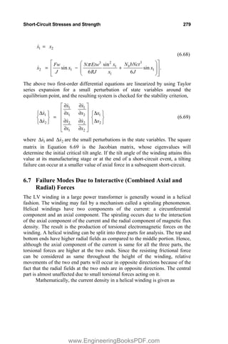
![280 Chapter 6
z z
J J
I I
J a a (6.70)
where J is the current density in A/m2
, JI and z
J are its circumferential and
axial components. The electromagnetic force density is produced in the
windings by the interaction of the current density J and the magnetic flux
density B. Mathematically,
0 .
0
r z
z z r z r r z
r z
J J J B J B J B
B B
I
I I I I
u
a a a
F J B a a a (6.71)
The first term on the right side gives the radial component of the force, the
second term in the circumferential direction represents the torsional force, and
the last term denotes the axial component of the force. Since the radial
component of the flux density Br is maximum at the winding ends, the torsional
forces are maximum at the ends. Practically also, it has been observed that in
helical windings the spiraling of conductors occurs at the ends. With an increase
in the helical angle the axial component of the current density increases, which
in turn increases the torsional (spiraling) forces. These forces produce
circumferential displacements of the helical winding [38].
The axial component of the current produces the azimuthal (I )
component of the magnetic flux density [39]. Although this component is lower
than the axial and radial components of the magnetic field, it is present in the
winding throughout its height. Although it does not contribute much to the eddy
loss in the winding, stray losses in nearby structural components can be
appreciable [39].
6.8 Effect of Prestress
The clamping pressure applied on the windings after the completion of core-
winding assembly is called prestress. It has a significant impact on the response
of windings during short circuits. Mechanical integrity of windings can be
ensured if a properly chosen prestress gets maintained throughout the life of the
transformers. If applied prestress is sufficient and maintained during the short-
circuit duration, it may rule out the onset of free buckling due to radial forces.
This is due to the transfer of axial prestress force to each disk through the radial
insulation spacers [28].
The prestress value should be chosen accurately to avoid an excited
resonance and large displacements of the windings. It has a significant effect in
deciding the natural frequencies of the windings and their oscillations. The
relationship between the natural frequencies and the prestress value can be
highly nonlinear [40]. A high value of prestress reduces oscillations of the
www.EngineeringBooksPDF.com](https://image.slidesharecdn.com/transformer-engineering-design-technology-and-diagnostics-second-edition-pdf-230506172819-680afe24/85/transformer-engineering-design-technology-and-diagnostics-second-edition-pdf-pdf-301-320.jpg)
![Short-Circuit Stresses and Strength 281
windings. It increases the stiffness of the overall system thereby increasing the
mechanical resonance frequencies. If an unprestressed natural frequency is
higher than the excitation frequencies, the oscillations are reduced at higher
values of the prestress. On the contrary, if the unprestressed natural frequency is
lower than the excitation frequencies, a higher value of the prestress may bring
them closer. Therefore, the prestress value should be judiciously chosen [19, 41,
42].
The above discussion assumes that the prestress value is constant;
however, it may change due to variations in temperature, presence of moisture in
insulation, and its aging. This will in turn affect the short-circuit performance of
the transformer. Any change in the thickness of the materials in the windings
and the end insulation regions will change the clamping pressure. Cellulose
insulation is organic in nature; its thickness and stiffness may change
appreciably over a period of time due to effects of temperature, moisture and
aging. Coefficients of thermal expansion of winding conductors, supporting
metallic structure and insulation are different; the coefficient for the insulation is
the greatest amongst them. Also, with an increase in temperature, (solid)
insulation material tends to shrink due to its decomposition processes.
Furthermore, with variations in temperature, there is continuous exchange of
moisture between oil and solid insulation. All these factors may reduce
ultimately the mechanical strength and stiffness of the insulation, and change the
natural frequencies; thus the problem of short-circuit withstand requires a
thorough understanding of all the involved physical phenomena. The natural
frequencies are reported to vary as a function of the square root of the ratio of
the prestress value to the maximum electromagnetic stress in the winding [19].
The natural frequency of a winding may change during the short-circuit
period due to changes in the insulation characteristics and the ratio of the
prestress to the total stress. Thus, the natural frequencies measured from the free
response may be different after a short circuit as compared to those measured
prior to the short-circuit event. Also, during the short circuit a winding, which
may be in resonance at some time experiencing a higher stress, may get detuned
from the resonance due to a change in insulation characteristics at some other
instant.
6.9 Short-Circuit Test
A short-circuit test can be performed by one of the following two techniques:
the preset short-circuit method and the post-set short-circuit method. In the pre-
set short-circuit test, a previously short-circuited transformer on its secondary
side is energized from the primary side. If the secondary winding is the inner
winding, the limb flux is low as explained in Section 5.12.2 (Figure 5.38)
resulting in an insignificant transient inrush current, and the method will work
well. If the primary winding is the inner one, there is substantial flux density in
www.EngineeringBooksPDF.com](https://image.slidesharecdn.com/transformer-engineering-design-technology-and-diagnostics-second-edition-pdf-230506172819-680afe24/85/transformer-engineering-design-technology-and-diagnostics-second-edition-pdf-pdf-302-320.jpg)
![282 Chapter 6
the limb and hence the inrush current is superimposed on the short-circuit
current. Since the inrush current flows through the primary winding only, it
creates a significant ampere-turn unbalance between the primary and secondary
windings resulting in high short-circuit forces. Depending upon the instant of
closing and the core residual flux, the magnitude of the inrush current varies (as
explained in Chapter 2). In order to reduce the inrush current and its effects
during the test, the core can be deliberately premagnetized with the opposite
polarity [43].
In the post-set short-circuit test method, the transformer is in the energized
condition and its secondary winding is short-circuited. Naturally, this method is
preferred as there are no inrush currents and the related problems, and also due
to the fact that the test circuit represents typical site conditions during faults.
However, the disadvantage of this method is that the short-circuit capacity of
test stations has to be much higher [9, 44] than that in the first method to
maintain the rated voltage across the transformer terminals (by overcoming the
voltage drop across the series impedance between the source and the
transformer) and establish the required value of the short-circuit current. If the
source impedance is not negligible as compared to the transformer impedance, a
higher voltage needs to be applied, subject to a limit of 1.15 p.u. on the no-load
source voltage according to IEC standard 60076-5 (third edition: 2006-02).
Thus, the required short-circuit capacity of the test station increases. The
capacity should be at least 9 times the short-circuit power of the transformer for
a 15% over-excitation condition [44]. The test stations may not have such
capability, and hence short-circuit tests on large transformers are usually carried
out by the pre-set method.
After the short-circuit test, the performance is considered satisfactory if
the following conditions are met according to the IEC standard:
- results of short-circuit tests and measurements performed during tests do not
indicate any condition of a fault
- routine tests including dielectric tests, repeated after the short-circuit test, are
successful
- out-of-tank inspection does not indicate any displacement/deformation of the
active part and/or support structures
- there are no traces of internal electrical discharges
- change in impedance is not more than 2% for any phase after the test for
transformers up to 100 MVA rating. The corresponding value is 1% for
ratings above 100 MVA. The more stringent requirement for large
transformers is in line with the experience that a variation in the impedance of
more than 1% in large power transformers indicates a large deformation in
one or more windings, whereas a change in the impedance between 0.5% to
1% indicates a progressive movement of winding conductors [43].
www.EngineeringBooksPDF.com](https://image.slidesharecdn.com/transformer-engineering-design-technology-and-diagnostics-second-edition-pdf-230506172819-680afe24/85/transformer-engineering-design-technology-and-diagnostics-second-edition-pdf-pdf-303-320.jpg)
![Short-Circuit Stresses and Strength 283
To evaluate test results, the most important and conclusive diagnostic test seems
to be the impedance measurement along with visual inspection [43], although
advanced techniques like FRA (frequency response analysis), vibration
measurements, dynamic oil pressure measurements, etc. are also used.
6.10 Effect of Inrush Current
As explained in Chapter 2, when a transformer is switched on, the magnitude of
its inrush current depends on many factors, the predominant factors being the
instant of switching and the residual magnetism in the core. The inrush current
can be as high as six to eight times the rated current, and transformer users are
always apprehensive about its repeated switching. Inrush transients are more
frequent than short circuits and they last for a few seconds compared to the short
circuits which are usually cleared in tens of milliseconds. The energized winding
is subjected to the mechanical stresses during an inrush transient. Inrush currents
are usually not taken very seriously from the mechanical design considerations.
Inner windings have a lower value of air-core reactance. Therefore, a
transformer switched from the inner winding experiences a higher inrush
current. It is well-known that layer/helical windings are vulnerable to short
circuits. Hence, if a transformer is switched on frequently from its inner
layer/helical winding, forces generated due to the inrush currents may make it
loose over a period of time; such a weakened winding becomes vulnerable
during a subsequent short circuit event. When a transformer is switched from the
outer HV winding having a higher air-core reactance value, the magnitude of the
inrush current and the corresponding forces are lower.
Recent insulation failures in larger transformers, which were frequently
energized under a no-load condition, have attracted attention of researchers. The
impact of inrush currents on mechanical stresses of windings has been
investigated in [45]. It is shown that the axial forces calculated with maximum
possible inrush currents are of the same order of magnitude as that calculated
with short-circuit currents, and hence the use of controlled switching strategies
is generally recommended. In another paper [46], the force patterns under the
short-circuit and inrush conditions are compared and shown to be significantly
different from each other.
6.11 Split-Winding Transformers
Split-winding transformers have the advantage that splitting secondary windings
into two parts obviates the need of having two double-winding transformers.
There is a considerable saving in instrumentation (on the HV side) and space,
since a transformer, with one HV winding and two LV windings, substitutes two
double-winding transformers of half the power rating.
www.EngineeringBooksPDF.com](https://image.slidesharecdn.com/transformer-engineering-design-technology-and-diagnostics-second-edition-pdf-230506172819-680afe24/85/transformer-engineering-design-technology-and-diagnostics-second-edition-pdf-pdf-304-320.jpg)
![284 Chapter 6
HV
HV2
HV1
LV2
LV1
Figure 6.16 Split-winding transformer.
The arrangement also results in a considerable reduction in the values of short-
circuit currents in the two separately supplied circuits, decreasing the required
rating of circuit breakers. The two LV windings are placed axially with respect
to each other in order to have equal impedances to the HV winding which is also
split into two parts with center-line lead arrangement as shown in figure 6.16.
The split-winding arrangement requires special short-circuit design
considerations. Consider the preset short-circuit method, in which a voltage is
applied to the HV winding with one of the LV windings, say LV2, short-
circuited. The flux density distribution is completely different in the lower and
upper parts of the core limb. The flux density in the upper part is high, requiring
a high value of magnetizing inrush current for the HV1 winding, whereas there
is no demand for a significant magnetizing current by the HV2 winding since
the flux density in the bottom part of the limb is very low due to the short-
circuited inner LV2 winding. This phenomenon results into heavy distortion of
fields in the core and windings of the transformer. There is considerable radial
field due to an asymmetrical distribution of ampere-turns resulting into
excessive axial forces and end thrusts.
The phenomenon is analyzed in [44] by means of a nonlinear magnetic
model. It is recommended to do two setup tests with opposite polarity to
magnetize the core in the reverse direction so that the inrush current is reduced
to a harmless value during the pre-set method. If the short-circuit capacity of the
test station is high enough to allow the post-set method (which eliminates the
inrush currents and related problems), there is still one more characteristic of the
split-winding transformer which makes the short-circuit test on it more severe
than that on a conventional two-winding transformer. With the LV2 winding
short-circuited, some current flows in the HV1 winding not facing directly the
short-circuited LV2 winding. The current in the HV1 winding is small, in the
range of 3 to 5% of that flowing in the HV2 winding [47] due to a much higher
www.EngineeringBooksPDF.com](https://image.slidesharecdn.com/transformer-engineering-design-technology-and-diagnostics-second-edition-pdf-230506172819-680afe24/85/transformer-engineering-design-technology-and-diagnostics-second-edition-pdf-pdf-305-320.jpg)
![Short-Circuit Stresses and Strength 285
impedance value between the HV1 and LV2 windings, but it is sufficient to
cause an ampere-turn unbalance along the height of the windings. The ampere-
turns of the HV2 winding are smaller than that of the LV2 winding, and
corresponding to the ampere-turns of the HV1 winding there are no balancing
ampere-turns in the LV1 winding (since it is open-circuited). Hence, there is a
considerable distortion of the leakage field resulting into higher axial short-
circuit forces [48]. For a given value of the short-circuit current, the forces are
higher for the case in which only one of the LV windings is short-circuited as
compared to the case when both LV windings are short-circuited. Thus,
although the split-winding configuration helps in limiting the rating of circuit
breakers, it poses problems for the short-circuit withstand.
The phenomenon has been accurately analyzed using coupled circuit-field
simulations in [49]. The short-circuit performance of a 70-MVA, three-phase,
220/6.9/6.9-kV transformer has been analyzed under the pre-set and post-set test
conditions. A 2-D axisymmetric field-circuit coupled nonlinear transient finite
element model has been developed for the purpose. Also, the beneficial effect of
deliberate pre-magnetization with opposite polarity is demonstrated.
6.12 Short-Circuit Withstand
The IEC 60076-5 (third edition: 2006-02) proposes that the ability to withstand
dynamic effects of short circuits should be demonstrated either by a short-circuit
test or by calculations/design considerations. The latter method is used if there
are constraints of cost, time, logistics and test limitations [25]. In this method,
the manufacturers need to provide calculations, technological choices and design
margins, and demonstrate the adequacy of manufacturing processes. They have
to validate dimensioning rules by reference to similar transformers which have
passed the test or by reference to the tests on representative models.
Comparisons of stress and strength values of the transformer with the
corresponding values of the reference transformers/models should be done. The
guidelines for identification of similar transformers are given in the IEC
standard. This method is a sort of comprehensive design verification with
involvement of the user to review material specifications, calculations of short-
circuit currents and stresses for various types of faults, safety margins and
quality control of manufacturing processes. The design review at different stages
of design and manufacturing is important in ensuring reliability of transformers
under short circuits. In order to improve the short-circuit performance of
transformers, the purchaser or his representative should be involved in
reviewing and assessing the quality of design and manufacturing processes at a
few important stages during the execution of the whole contract. There is a lot of
scope for cooperation between the transformer manufacturer and purchaser. Two
major areas for cooperation are technical specifications and design review. In
many cases, the purchaser may have confidence about the capability of the
manufacturer based on the design review and the results of short-circuit tests on
www.EngineeringBooksPDF.com](https://image.slidesharecdn.com/transformer-engineering-design-technology-and-diagnostics-second-edition-pdf-230506172819-680afe24/85/transformer-engineering-design-technology-and-diagnostics-second-edition-pdf-pdf-306-320.jpg)
![286 Chapter 6
model coils as well as full-sized transformers over a period of time. Guidelines
for the demonstration of the ability of transformers to withstand dynamic effects
of a short circuit are given in the IEC standard.
A short-circuit test is preferred by many purchasers to ascertain the short-
circuit performance of transformers. This is because the transformer is a highly
labor-intensive product and the short-circuit performance may be greatly
influenced by the quality of manufacturing processes. The transformer consists
of different kinds of materials whose responses to short-circuit forces are
different. Two transformers having an identical design may perform differently
during the short-circuit tests if the quality of manufacturing processes is not
consistent. Weaknesses in design and manufacturing processes are exposed
when there is a failure during the test, which may disclose some intricate failure
modes based on which design and manufacturing processes can be improved. It
should be remembered that, in addition to a detailed theoretical analysis with the
help of advanced computational techniques, it is very much essential to correlate
the results of calculations with the experimental data of short-circuit tests on
transformers or their equivalent models. These tests give authentic confirmation
of the assumptions or estimates of material properties, transfer of forces,
clearances, etc., used in the theoretical analysis.
There are many influencing factors that determine the short-circuit stresses
and withstand. These factors along with general guidelines and precautions, that
can be taken at the specification, design, and production stages of transformers,
are described below.
6.12.1 System configuration and transformer specification [1]
1. Limited extension of subtransmission networks thereby reducing short-
circuit levels in the system.
2. High impedance grounding of the neutral of distribution and sub-
transmission networks.
3. Specification of higher values of percentage impedances for critical
transformers.
4. Use of transformers instead of autotransformers, if possible, even if it
results in a higher cost.
5. Neutral end taps for transformers with on-load tap changing arrangement.
6. Specification of taps on more than one winding should be avoided.
7. Lower tapping range.
8. Removal of stabilizing tertiary winding from the specification for three-
phase three-limb transformers up to a certain rating.
9. Specification and use of the split-winding configuration should be avoided,
if possible.
The above recommendations have an impact on the power system protection and
performance; hence they should be adopted after a thorough study.
www.EngineeringBooksPDF.com](https://image.slidesharecdn.com/transformer-engineering-design-technology-and-diagnostics-second-edition-pdf-230506172819-680afe24/85/transformer-engineering-design-technology-and-diagnostics-second-edition-pdf-pdf-307-320.jpg)
![Short-Circuit Stresses and Strength 287
6.12.2 Design
1. If the stabilizing tertiary winding is essential, its current density should be
as low as possible (i.e., a massive and stiff winding).
2. For withstanding radial forces, the conductor dimensions can be chosen in
such a way that the conductor can resist the compressive forces on its own,
without relying on its supporting structures.
3. Whenever a CTC conductor is used for achieving lower winding stray
losses and for the ease of winding, it should be epoxy-bonded to greatly
enhance the resistance of the winding against buckling and tilting.
4. Windings can be made of high proof stress conductor material.
5. Use of lower current densities in windings of critical transformers.
6. Use of thicker insulating cylinders for supporting inner windings.
7. Adoption of a high slenderness ratio for the inner winding to increase its
compressive strength against the radial forces.
8. Estimation of natural frequencies of windings and ensuring that there is no
excited resonance.
9. Correct selection of winding arrangements to minimize short-circuit forces.
10. It is usually preferable to have taps in a separate winding and not in the
body of the main winding from the short-circuit strength consideration.
Further, the turns should be so arranged in the separate tap winding that
when one tap-step is cut out of the circuit, the turns are uniformly removed
along the height of the winding (e.g., the interleaved tap winding shown in
Figure 7.15), minimizing the ampere-turn unbalance between the LV and
HV windings along their height.
11. If the taps need to be provided in the body of the HV winding, their
placement at its ends should be avoided. The short-circuit forces are
reduced when the taps are put in the center. The forces are further reduced if
they are put in two groups in the body and placed symmetrically about the
center line of the winding. A relative comparison of short-circuit forces for
various arrangements of tap positions is given in [10] using residual
ampere-turn diagrams. The ampere-turns of the untapped winding should be
reduced in the region corresponding to the tapping zone of the tap winding.
The balancing of ampere-turns between the LV and HV windings in this
zone should be done at the average tap position.
6.12.3 Manufacturing processes
1. Proper alignment of axially placed spacers to give adequate support to inner
windings.
2. Accurate positioning of axial and radial support structures.
3. A winding should be wound tightly on the axial spacers placed on the
cylinder, in which case a sufficiently thick cylinder can provide significant
support to the winding for withstanding the forces that tend to buckle it.
www.EngineeringBooksPDF.com](https://image.slidesharecdn.com/transformer-engineering-design-technology-and-diagnostics-second-edition-pdf-230506172819-680afe24/85/transformer-engineering-design-technology-and-diagnostics-second-edition-pdf-pdf-308-320.jpg)
![288 Chapter 6
4. Place tight-fitting wooden dowels on the core in close contact with the
insulating cylinders, and radially in line with the axial supports.
5. Before use, special storage conditions are required for epoxy-bonded CTC
conductors as per the supplier’s instructions. Also, it is a good practice to
cut a sample of the CTC conductor used for the winding, process it along
with the winding, and then check its mechanical properties through a
suitable testing procedure [5].
6. Strictly control manufacturing processes for windings.
7. When a double-layer winding is used to have an advantage of field
cancellation due to go-and-return conductors (which reduces the associated
stray losses), short-circuit forces are high both at the winding terminations
and also in the leads. Hence, adequate precautions need to be taken for
improving the short-circuit withstand at lead take-off points and also at the
terminations. For a single-layer winding, one connection is made at the top
and the other at the bottom of the winding resulting in manageable values of
forces. But in this case, the route of high current leads from the winding
bottom should be carefully designed to minimize the stray losses as they run
parallel to the tank and other structural components before terminating on
the tank cover at the top.
8. Purchase of materials from qualified suppliers with clear material
specifications and quality assurance procedures.
9. Use of high density pressboard for insulation components within windings,
and between windings and yokes.
10. Judicious selection of the prestress value and tight control on heights of
windings with no magnetic asymmetry between them.
11. Use of clamping structures having adequate stiffness with appropriate
fastening.
12. Adequate securing of leads at winding ends.
13. Adequate fastening of connections to the tap-changer and bushings.
14. Use of fiberglass reinforced clamping rings, if required.
15. Winding cylinders made of fiberglass can be used for inner windings.
16. Use of preshrunk and oil-impregnated special insulation components (e.g.,
angle rings/spacers).
17. Vapor phase drying of windings before the final assembly in specific cases
for better dimensional control.
18. Burr-free edge rounding of spacers for eliminating the biting of the paper
insulation on winding conductors.
19. Ensuring tightness of conductors in the radial direction.
20. For better sizing, windings are individually processed (heating and vacuum
cycles) followed by an axial compression before the final assembly, which
minimizes the possibility of any looseness in them. The designed winding
height should be obtained at the final assembly stage before applying the
final clamping pressure, which is achieved by inserting/removing insulation
spacers (blocks).
www.EngineeringBooksPDF.com](https://image.slidesharecdn.com/transformer-engineering-design-technology-and-diagnostics-second-edition-pdf-230506172819-680afe24/85/transformer-engineering-design-technology-and-diagnostics-second-edition-pdf-pdf-309-320.jpg)

![290 Chapter 6
For rectangular conductors, an accurate force calculation is possible by
considering the conductor cross section as a superimposition of interacting line
current filaments. The force per unit length between parallel rectangular
conductors shown in Figure 6.17 (b), for which l d, is
s
k
d
i
i
f 2
1
7
10
2
u N/m (6.74)
where ,
s
k a function of ¸
¹
·
¨
©
§
b
a
b
d
, is the shape factor that varies according to
the dimensions and the spacing between the conductors. The value of s
k for
different values of a, b and d can be obtained from the curves given in [50, 51].
In transformers, rectangular conductors/flats are used between windings
and terminations. These conductors have to be supported at regular intervals to
withstand short-circuit forces. Consider a rectangular conductor subjected to an
electromagnetic force acting uniformly on it. Let the distance between two
consecutive supports be S. The conductor structure, subjected to short-circuit
loads, acts as a beam supported at both ends as shown in Figure 6.18. The
maximum bending moment is
12
2
S
f
M (6.75)
where f is the load (force) per unit length (to be calculated by Equation 6.74).
0000
0000
1111
1111
f S2
24
S
b
a
Fixed
Conductor
cross section
support
Configuration
f
Bending moment diagram
f S2
12
+ve
Ŧve
+ve
Figure 6.18 Calculation of maximum unsupported span.
www.EngineeringBooksPDF.com](https://image.slidesharecdn.com/transformer-engineering-design-technology-and-diagnostics-second-edition-pdf-230506172819-680afe24/85/transformer-engineering-design-technology-and-diagnostics-second-edition-pdf-pdf-311-320.jpg)
![Short-Circuit Stresses and Strength 291
Now,
y
I
M V
(6.76)
where
12
3
a
b
I is the moment of inertia,
2
a
y is the maximum distance from
the neutral axis for the conductor, and V is the stress in the conductor. By
putting the values of M, I and y in Equation 6.76 we obtain
2
2
2
N/m
2
f S
b a
V . (6.77)
If max
V is the maximum allowable stress in the conductor in N/m2
, substituting
the value of f from Equation 6.74 for the same current i (the peak value of an
asymmetrical current) flowing in the two parallel conductors, we obtain the
expression for the maximum allowable spacing between the consecutive
supports of the conductor as
s
max
k
d
b
i
a
S
V
7
10
1u meters. (6.78)
Similarly, the maximum allowable spacing between the supports of a
rectangular conductor for any other support condition can be determined.
The analysis given above is applicable for a rectilinear conductor. For
more complex arrangements (e.g., bends in a conductor or two conductors in
different planes), analytical formulations are possible [52]. However, any
complex arrangement of conductors can be easily analyzed now using FEM.
6.14 Design of Clamping Structures
The clamping structures are provided in a transformer to prevent any movement
of windings due to the forces produced at the time of a short circuit. Therefore,
the clamping structures are designed such that they put the windings under a
desired pressure condition. The clamping structures consist of the clamping ring,
flitch plates and frames, as shown in Figure 6.19.
Stresses in clamping ring:
Bolts are provided for maintaining a constant pressure on the windings; the
required pressure is applied on the clamping ring by tightening the bolts in small
transformers. For large transformers, the pressure is usually applied by hydraulic
jacks, and the bolts are then locked in positions or fiberglass/densified wood
wedges are inserted. Under short-circuit conditions, the forces produced in the
windings try to bend the portion of the ring between two consecutive bolts. The
www.EngineeringBooksPDF.com](https://image.slidesharecdn.com/transformer-engineering-design-technology-and-diagnostics-second-edition-pdf-230506172819-680afe24/85/transformer-engineering-design-technology-and-diagnostics-second-edition-pdf-pdf-312-320.jpg)


![300 Chapter 7
of oscillations. When the applied voltage is maintained for a sufficiently long
time (50 to 100 microseconds), appreciable currents begin to flow in the
inductances eventually leading to the uniform voltage distribution. Since there is
difference between the initial and final voltage distributions, as shown in Figure
7.1, a transient phenomenon takes place. During this transient period, there is
continual interchange of energy between electric and magnetic fields. On
account of a low damping factor of the transformer windings, the transient is
oscillatory. The voltage at any point in the winding oscillates about the final
voltage value, reaching a maximum as shown by curve c. It is obvious that the
strength of the transformer windings to lightning voltages can be significantly
increased if the difference between the initial and final distributions can be
minimized. This not only reduces the excessive stresses at the line end but also
mitigates the oscillations thereby keeping the voltage to ground at any point in
the winding insignificantly higher than the final voltage distribution.
The differential equation governing the initial voltage distribution
),
0
,
(
0 x
u
u for the representation of a winding shown in Figure 7.2 (wherein
inductive effects are neglected), is [1]
0
0
2
0
2
u
c
c
dx
u
d
s
g
. (7.1)
In Figure 7.2, s
L , cg and cs denote the self inductance per unit length, the shunt
capacitance per unit length to ground, and the series capacitance per unit length
between adjacent turns, respectively.
%
of
applied
voltage
a
b
20
40
80
100
60
0
100 80 60 40 20 0
% of winding height
c
line
end
neutral
end
(a) initial distribution (b) final distribution (c) maximum voltage to ground
Figure 7.1 Impulse voltage distribution.
www.EngineeringBooksPDF.com](https://image.slidesharecdn.com/transformer-engineering-design-technology-and-diagnostics-second-edition-pdf-230506172819-680afe24/85/transformer-engineering-design-technology-and-diagnostics-second-edition-pdf-pdf-321-320.jpg)


![Surge Phenomena in Transformers 305
given by Equation 7.15, with s equal to half the value of the distance between
the axes of the two windings (refer to Equation D28).
7.3 Capacitance of Windings
7.3.1 Development of winding methods for better impulse response
In the initial days of transformer technology development for higher voltages,
the use of electrostatic shields was quite common (see Figure 7.4). A non-
resonating transformer with electrostatic shields was reported in [2, 3, 4]. It is a
very effective shielding method in which the effect of the ground capacitance of
an individual section is neutralized by the corresponding capacitance to the
shield. Thus, the currents in the shunt (ground) capacitances are supplied from
the shields and none of them have to flow through the series capacitances of the
winding. If the series capacitances along the windings are made equal, uniform
initial voltage distribution can be achieved. The electrostatic shield is at the line
terminal potential and hence must be insulated from the winding and the tank
along its height. As voltage ratings and corresponding dielectric test levels
increased, it became increasingly difficult and cumbersome to design the
shields. They were found to be less cost effective since extra space and material
were required for insulating shields from other electrodes inside the transformer.
Subsequent development of interleaved windings phased out completely the use
of electrostatic shields. However, the principle of electrostatic shielding is
regularly used in the form of static end rings at the line end of high voltage
windings and static rings within the windings, which improve the voltage
distributions and reduce the stresses locally.
cs
cg
Shield
Figure 7.4 Electrostatic shields.
www.EngineeringBooksPDF.com](https://image.slidesharecdn.com/transformer-engineering-design-technology-and-diagnostics-second-edition-pdf-230506172819-680afe24/85/transformer-engineering-design-technology-and-diagnostics-second-edition-pdf-pdf-326-320.jpg)
![306 Chapter 7
10 9 8 7 6 5 4 3 2 1
11 12 13 14 15 16 17 18 19 20
30 29 28 27 26 25 24 23 22 21
31 32 33 34 35 36 38 39 40
37
winding
cylinder
spacer
line end
Figure 7.5 Continuous winding.
In order to understand the effectiveness of an interleaved winding, let us
first analyze a continuous (disk) winding shown in Figure 7.5. The total series
capacitance of the continuous winding is an equivalent of all turn-to-turn and
disk-to-disk capacitances. Although the capacitance between two adjacent turns
is high, all the turn-to-turn capacitances are in series, which results in a much
smaller capacitance value for the entire winding. Similarly, all disk-to-disk
capacitances which are also in series, add up to a small value. With an increase
in the voltage class, the insulation between turns and between disks has to be
increased which further worsens the total series capacitance.
An inherent disadvantage of a low series capacitance value of the
continuous winding was overcome by electrostatic shielding as explained earlier
until the advent of the interleaved winding. The original interleaved winding
was introduced and patented by G. F. Stearn in 1950 [5]. A simple disposition of
turns in some particular ways increases the series capacitance of the interleaved
winding to such an extent that near uniform initial voltage distribution can be
obtained. A typical interleaved winding is shown in Figure 7.6.
1
40
winding
cylinder
spacer
line end
6
14
5
15
35 24 21
31
26 36 27
2 11
12
13
4
19 10 20
25 34 33 23 32 22
39 30
29
38
28
37
3
9
18
8
17
7
16
Figure 7.6 Interleaved winding.
www.EngineeringBooksPDF.com](https://image.slidesharecdn.com/transformer-engineering-design-technology-and-diagnostics-second-edition-pdf-230506172819-680afe24/85/transformer-engineering-design-technology-and-diagnostics-second-edition-pdf-pdf-327-320.jpg)
![Surge Phenomena in Transformers 307
In an interleaved winding, two consecutive electrical turns are separated
physically by a turn which is electrically much farther along the winding. It is
wound as a conventional continuous disk winding but with two conductors. The
radial position of the two conductors is interchanged through a crossover
between them at the inside diameter and appropriate conductors are joined at the
outside diameter, thus forming a single circuit two-disk coil. The advantage is
obvious since it does not require any additional space as in the case of complete
electrostatic shielding or part electrostatic shielding (static rings). In interleaved
windings, not only the series capacitance is increased significantly but the
ground capacitance is also somewhat reduced because of improvement in the
winding space factor. This is because the insulation within the winding in the
axial direction can be reduced due to improvement in the voltage distribution,
which reduces the winding height and hence the ground capacitance. Therefore,
the distribution constant (D ) is reduced significantly lowering stresses between
various parts of the winding.
It can be seen from Figure 7.6 that the normal working voltage between
adjacent turns in an interleaved winding is equal to voltage per turn times the
turns per disk. Hence, one may feel that a much higher amount of turn insulation
may be required, thus questioning the effectiveness of the interleaved winding.
However, due to significant improvement in the voltage distribution, stresses
between turns are reduced by a great extent so that the percent safety margins
for the impulse stress and the normal working stress can be made of the same
order. Hence, the turn-to-turn insulation is used in an effective way [6]. Since
the voltage distribution is more uniform, the number of special insulation
components (e.g., disk angle rings) along the winding height reduces. When a
winding has more than one conductor per turn, the conductors are also
interleaved as shown in Figure 7.7, for a winding with 6 turns per disk and two
parallel conductors per turn, to obtain maximum benefit.
spacer
1A
2A
3A
4A
7A
8A
9A 1B
7B
2B
8B
3B
9B
4B 5B 6B
10A 10B 6A
11A 11B 12A 12B
21B 15B 21A 15A 20B 14B 20A 14A 19B 13B 19A 13A
16A 22A 16B 22B 17A 23A 17B 23B 18A 24A 18B 24B
5A
winding
cylinder
Figure 7.7 Interleaving with 2-parallel conductors per turn.
www.EngineeringBooksPDF.com](https://image.slidesharecdn.com/transformer-engineering-design-technology-and-diagnostics-second-edition-pdf-230506172819-680afe24/85/transformer-engineering-design-technology-and-diagnostics-second-edition-pdf-pdf-328-320.jpg)
![308 Chapter 7
3 1
4 2
5
15 14 13 12 11
6 17 7 8 9 20 10
16 18 19
3 1
6 7 8 9 10
4 2
5
15 14 13 12 11
16 17 18 19 20
(a) Stern winding (b) Nuys winding
Figure 7.8 Two types of crossovers in interleaved winding.
In [7], the reason for improved surge characteristics of interleaved
windings is explained using transmission line-like representation of the disks.
There can be two types of interleaved windings with regard to the crossover
connections at the inside diameter as shown in Figure 7.8. When steep impulse
waves such as chopped waves or front-of-waves enter an interleaved winding, a
high oscillatory voltage appears locally between turns at the center of the radial
build of the disk. This phenomenon is analyzed in [8, 9] for these two types of
crossovers used in the interleaved windings.
7.3.2 Turn-to-turn and disk-to-disk capacitances
For determining series capacitances of different types of windings, the
calculations of turn-to-turn and disk-to-disk capacitances are essential. The turn-
to-turn capacitance is given by
p
p
m
p
T
t
t
w
D
C
)
(
0
uS
H
H
(7.16)
where m
D is the average diameter of the winding, w is the bare width of the
conductor in the axial direction, p
t is the total paper insulation thickness (both
sides), 0
H is the permittivity of free space, and p
H is the relative permittivity of
the paper insulation. The term p
t has been added to the conductor width to take
into account fringing effects.
Similarly, the total axial capacitance between two consecutive disks based
on geometrical considerations only is given by
s
m
s
s
p
p
oil
s
p
p
DA t
R
D
t
t
k
t
t
k
C
u
»
»
¼
º
«
«
¬
ª
S
H
H
H
H
H
1
0 (7.17)
where R is the winding radial depth, s
t and s
H is the thickness and the relative
permittivity of the solid insulation (radial spacers between disks) respectively,
and k is the ratio of the area occupied by the oil to the total circumferential
area. The term s
t is added to R to take into account fringing effects.
www.EngineeringBooksPDF.com](https://image.slidesharecdn.com/transformer-engineering-design-technology-and-diagnostics-second-edition-pdf-230506172819-680afe24/85/transformer-engineering-design-technology-and-diagnostics-second-edition-pdf-pdf-329-320.jpg)
![Surge Phenomena in Transformers 309
For the continuous winding and its variations (with static end rings/static
rings between disks), there are two approaches for calculating the series
capacitance. In the first approach, the voltage is assumed to be evenly
distributed within the disk winding, which makes the calculation easy. However,
this is a major approximation for continuous disks having low effective interturn
series capacitance. The second approach, in which linear voltage distribution is
not assumed within the disks for the capacitance calculation, is accurate [10, 11,
12]. The corresponding representation of capacitances for this method is shown
in Figure 7.9. The total series capacitance of the winding is given by [10, 13]
d
d
DA
DW
d
d
DA
d
d
DA
d
d
DA
S
C
N
C
C
C
C
D
D
D
D
D
D
D
D
2
tanh
2
2
2
tanh
4
2
tanh
2
2
tanh
2
»
»
¼
º
«
«
¬
ª
»
¼
º
«
¬
ª
(7.18)
where DA
C = disk-to-disk capacitance calculated based on geometrical
considerations
d
D = distribution constant of a disk =
)
1
(
D
T
DA
N
C
C
T
C = turn-to-turn capacitance
D
N = number of turns per disk
DW
N = number of disks in the winding.
equipotential
surfaces
/N
C
2
C /2
C /2
T
T
DA D
CT
Figure 7.9 Representation of capacitances of a continuous winding.
www.EngineeringBooksPDF.com](https://image.slidesharecdn.com/transformer-engineering-design-technology-and-diagnostics-second-edition-pdf-230506172819-680afe24/85/transformer-engineering-design-technology-and-diagnostics-second-edition-pdf-pdf-330-320.jpg)

![Surge Phenomena in Transformers 311
Now, the voltages across the first, second, and third interdisk capacitances
( D
C ) from the inside diameter are
2
2 D
V
N
§ ·
¨ ¸
© ¹
,
4
2 D
V
N
§ ·
¨ ¸
© ¹
, and ¸
¸
¹
·
¨
¨
©
§
D
N
V
2
6
, respectively.
Hence, the expression for the voltage across D
C at the outside diameter is
D
D
N
V
N
2
1
2 . The total energy stored by all such capacitances is
»
»
¼
º
«
«
¬
ª
¸
¸
¹
·
¨
¨
©
§
¸
¸
¹
·
¨
¨
©
§
¸
¸
¹
·
¨
¨
©
§
¸
¸
¹
·
¨
¨
©
§
2
2
2
2
2
1
2
2
6
2
4
2
2
2
1
D
D
D
D
D
D
N
V
N
...
N
V
N
V
N
V
C
En .
(7.20)
Simplifying and using the identity:
6
)
1
2
)(
1
(
)
1
(
3
2
1 2
2
2
2
˜
˜
˜
˜
n
n
n
n
we obtain
2
2
2
1
12
1
2
1
V
C
N
V
C
N
N
En DR
D
D
D
D
(7.21)
where DR
C is the resultant interdisk capacitance.
D
D
D
D
DR
N
C
N
N
C
6
1
2
1
? . (7.22)
Instead of using the lumped parameter approach for the interdisk capacitances, if
they are represented by a distributed capacitance DU
C (i.e., capacitance per unit
radial depth based on the geometrical considerations only), the value of the
resultant interdisk capacitance for a radial depth of R can be calculated as [14]
3
3
DA
DU
DR
C
R
C
C . (7.23)
The previous two Equations are equivalent, because if the number of turns per
disk is much greater than 1 ( 1
!!
D
N ), Equation 7.22 becomes
3
3 /
R
C
/
C
N
C DU
D
D
DR # .
The resultant series capacitance of the disk pair is given as the addition of the
resultant interturn capacitance and the resultant interdisk capacitance,
1
2
1
6
1
2 2
D
D
D
D
D
D
T
se N
N
N
C
N
N
C
C (7.24)
www.EngineeringBooksPDF.com](https://image.slidesharecdn.com/transformer-engineering-design-technology-and-diagnostics-second-edition-pdf-230506172819-680afe24/85/transformer-engineering-design-technology-and-diagnostics-second-edition-pdf-pdf-332-320.jpg)

![Surge Phenomena in Transformers 313
By providing a large equipotential surface with a good corner radius, SER
reduces the stress concentration at the line end. It also improves the effective
series capacitance at the line end as explained below. The closer the location of
SER to the line end disk, the greater the increase in the series capacitance value
is. This results in reduction of stresses appearing within the line end disk.
Let us calculate the series capacitance of a disk pair with SER as per the
method given in [14]. SER is usually connected to the first turn of the winding
by means of a pig-tail; hence the potential of SER is fixed to that of the line
terminal (V) as shown in Figure 7.12. Let the winding radial depth be denoted by
R.
The voltage at any point x of the upper section representing SER is
V
x
V )
(
1 (7.30)
and the voltage at any point x of the lower section representing the first disk is
R
x
R
V
R
x
R
V
V
x
V
2
2
2
2
2
»
¼
º
«
¬
ª
. (7.31)
Let SU
C be the capacitance between SER and the first disk per unit depth of the
winding (based on the geometrical considerations only). Therefore, the energy
stored in the capacitance SU
C per unit depth at point x is
@2
2
1 )
(
)
(
2
1
x
V
x
V
C
En SU
x . (7.32)
V1
V/2
V
V
V2 (x)
(x)
x
0
0
0
V/2
V
R
Figure 7.12 Calculation of the capacitance between SER and the line end disk.
www.EngineeringBooksPDF.com](https://image.slidesharecdn.com/transformer-engineering-design-technology-and-diagnostics-second-edition-pdf-230506172819-680afe24/85/transformer-engineering-design-technology-and-diagnostics-second-edition-pdf-pdf-334-320.jpg)


![316 Chapter 7
necessitating the use of a large number of parallel conductors for controlling the
winding eddy loss. An interleaved winding with a large number of parallel
conductors is difficult from the productivity point of view. Hence, shielded-
conductor (wound-in-shields) technology is adopted in high voltage windings of
large power transformers. This is because the continuously transposed cable
(CTC) conductor, which is ideally suited for such applications (as explained in
Chapter 4), can be used with this technology.
7.3.6 Shielded-conductor winding
A shielded-conductor winding gives a modest but sufficient increase in the
series capacitance and is less labor intensive as compared to an interleaved
winding. The number of shielded conductors can be gradually reduced in the
shielded disks from the line end, giving a possibility of achieving a tapered
capacitance profile to match the voltage stress profile along the winding height
[15]. This type of winding has some disadvantages, viz. reduction in the winding
space factor, requirement of extra winding material (shields), disturbance in
ampere-turn balance per unit height of the LV and HV windings, and an extra
eddy loss in the shields.
Let us calculate the total series capacitance of a shielded-conductor disk-
pair shown in Figure 7.13. For D
N turns per disk with an applied voltage of V
across the disk-pair, the voltage per turn is ).
2
( D
N
V It is assumed that for
shields also, the same value of voltage per turn is applicable. Out of D
N turns,
the first k turns are shielded in each disk. The shield can be either floating or it
can be connected to some turn. Here, the shield conductors are assumed to be
floating. For the first disk the voltage of any turn is
D
D
c N
i
N
V
i
V
i
V ,
,
2
,
1
2
)
1
(
)
(
. (7.41)
The voltage of ith
shield turn is (the 1st
shield takes the average potential of V/2):
k
i
N
V
i
V
i
V
D
s ,
,
2
,
1
2
)
1
(
2
)
(
. (7.42)
ND
ND
ND
ND ND
ND
ND
V
V
1
1
2
2
3
3
Ŧ 1
+ +
1 2 2 Ŧ 2 Ŧ1 2
1
2
2
3
0
k
k
Figure 7.13 Shielded-conductor winding.
www.EngineeringBooksPDF.com](https://image.slidesharecdn.com/transformer-engineering-design-technology-and-diagnostics-second-edition-pdf-230506172819-680afe24/85/transformer-engineering-design-technology-and-diagnostics-second-edition-pdf-pdf-337-320.jpg)

![318 Chapter 7
using which the effective capacitance of the disk-pair can be calculated. A
similar procedure can be followed if, through an electrical connection, the shield
is attached to some potential instead of being in the floating condition. The
calculation of capacitances of a shielded-conductor winding has been verified in
[15] by a circuit model and also by measurements on a prototype model.
7.3.7 Layer winding
For a simple layer (spiral) winding shown in Figure 7.14, wherein an individual
turn may have a number of parallel conductors depending upon the current
rating, the series capacitance can be determined as follows.
Let T
C be the interturn (turn-to-turn) capacitance and W
N be the total
number of turns in the winding. As before, the voltage is assumed to be
uniformly distributed within the winding. The energy stored in the winding is
equal to the sum of the energies stored in the individual capacitances,
2
2
2
1
1
2
1
V
C
N
N
V
C
En S
W
W
T
¸
¸
¹
·
¨
¨
©
§
. (7.51)
winding
layer
N
C
N
N
C
C
W
T
W
W
T
S
#
? 2
1
. (7.52)
For a helical winding (a layer winding with radial spacers between turns), the
above equation applies with T
C calculated by using Equation 7.16 with the
consideration of the proportion of the area occupied by the spacers (solid
insulation) and the oil.
7.3.8 Interleaved tap winding
In high-voltage high-rating transformers, when a spiral winding is used as a tap
winding, the tap sections are interleaved as shown in Figure 7.15. The tap
winding consists of 8 circuits (steps) giving a voltage difference between
adjacent turns either corresponding to a one-circuit difference or a two-circuit
difference. Thus, if there are 10 turns per circuit, the voltage difference between
touching turns is either equal to 10 or 20 times the voltage per turn. This higher
voltage difference necessitates the use of higher paper insulation reducing the
interturn capacitance, but the reduction is more than compensated by an
increased capacitive effect due to a higher voltage between the turns.
1 2 3 4 W
N
Figure 7.14 Layer winding.
www.EngineeringBooksPDF.com](https://image.slidesharecdn.com/transformer-engineering-design-technology-and-diagnostics-second-edition-pdf-230506172819-680afe24/85/transformer-engineering-design-technology-and-diagnostics-second-edition-pdf-pdf-339-320.jpg)
![Surge Phenomena in Transformers 319
1 3 5 7 8 6 4 2 1 3 5 7 8 6 4 2
first turn second turn
winding cylinder
spacer
. . . . .
Figure 7.15 Interleaved tap winding.
Let us calculate the value of series capacitance of an interleaved winding
having 8 circuits with 10 turns per circuit, giving a total number of 80 turns for
the tap winding. Assuming again that the voltage is uniformly distributed within
the tap winding with the voltage per turn as ,
80
V the energy stored in the
winding is
°
¿
°
¾
½
°̄
°
®
¸
¹
·
¨
©
§
u
°
¿
°
¾
½
°̄
°
®
¸
¹
·
¨
©
§
u
»
»
¼
º
«
«
¬
ª
¸
¹
·
¨
©
§
u
u
2
2
2
80
9
2
1
9
80
10
2
1
80
10
2
2
1
6
10
V
C
V
C
V
C
En T
T
T .
(7.53)
Simplifying and equating it to ,
2
/
1 2
V
CS we obtain the effective series
capacitance of the interleaved tap winding as
T
S C
C 4
# . (7.54)
Comparing this value of the series capacitance with that of the layer winding
having 80 turns as given by Equation 7.52, it can be seen that the series
capacitance has increased by about 320 times. The series capacitance for any
other interleaved tap winding, with different turns per circuit and number of
circuits, can be easily calculated by following the above procedure.
The method presented until now for the calculation of series capacitance
of windings is based on the stored energy. There are few other methods reported
in the literature. A rigorous analytical method is presented in [16] to calculate
the equivalent series capacitance of windings. The method is also used to
determine natural frequencies and internal oscillations of windings.
Analytical methods have a disadvantage that fringing effects and
corresponding stray capacitances cannot be accurately taken into account. In this
respect, numerical methods like FEM can give an accurate value of the
capacitance. In the FEM analysis also, the capacitance is calculated from the
stored energy (En) as
2
2
V
En
C . (7.55)
The procedure is similar to that of the leakage inductance calculation by
the FEM analysis as described in Chapter 3.
www.EngineeringBooksPDF.com](https://image.slidesharecdn.com/transformer-engineering-design-technology-and-diagnostics-second-edition-pdf-230506172819-680afe24/85/transformer-engineering-design-technology-and-diagnostics-second-edition-pdf-pdf-340-320.jpg)
![320 Chapter 7
A B
12 1 p.u
0.5
3
C
D
0 p.u
0.5
6
Figure 7.16 Capacitance calculation by FEM analysis.
The series capacitance of a disk-pair of a continuous disk winding and an
interleaved winding is now calculated by FEM for the geometry shown in Figure
7.16 (dimensions are in mm). The gap between the two disks is 6 mm. There are
6 turns per disk, and uniform voltage distribution is assumed. The relative
permittivities of oil and paper insulation are taken as 2.2 and 3.5, respectively.
The geometry is enclosed in a rectangular boundary at a distance of 1 meter
from the disks on all sides, so that the boundary conditions do not affect the
potential distribution in the disks. The energy is calculated for the rectangular
area ABCD. The values of the capacitance per unit length calculated by the
analytical formulae (Equations 7.25 and 7.40) and the FEM analysis are given in
Table 7.1.
7.4 Inductance Calculation
The insulation design based on only initial voltage distribution (with inductances
neglected) may be acceptable for transformers of smaller voltage ratings. The
difference between the initial and final (linear) distributions sets up oscillations
in the winding. According to Weed’s principle [17], a winding will be non-
oscillating if the capacitive (initial) and inductive (final) distributions are alike;
otherwise the difference will set up an oscillation under conditions favorable to
it, and such an oscillation may result into much larger voltage gradients between
different parts of the winding. Hence, the voltage distribution under impulse
conditions should be calculated with the inclusion of inductances in the winding
representation.
Table 7.1 Capacitance Calculation by Analytical Method and FEM Analysis
Continuous
winding
Interleaved
winding
Analytical 57.4 pF/m 1006.8 pF/m
FEM 61.8 pF/m 1073.4 pF/m
www.EngineeringBooksPDF.com](https://image.slidesharecdn.com/transformer-engineering-design-technology-and-diagnostics-second-edition-pdf-230506172819-680afe24/85/transformer-engineering-design-technology-and-diagnostics-second-edition-pdf-pdf-341-320.jpg)
![Surge Phenomena in Transformers 321
The mutual inductance between two coaxial coil loops (A and B) of radii
A
R and B
R with a distance S between them is given in SI units as [15, 18, 19]
°
¿
°
¾
½
°̄
°
®
»
»
¼
º
«
«
¬
ª
)
(
)
(
2
1
2 2
0
k
E
k
K
k
R
R
N
N
k
L B
A
B
A
AB
P
(7.56)
where
2
2
4
S
R
R
R
R
k
B
A
B
A
(7.57)
and A
N and B
N are the turns in sections A and B respectively, whereas )
(k
K
and )
(k
E are the complete elliptic integrals of the first and second kinds
respectively. The formula is applicable for thin circular filaments of negligible
cross section. For circular coils of rectangular cross section, more accurate
calculations can be done by using Lyle’s method in combination with Equation
7.56 [20, 21].
The self inductance of a single turn circular coil of square cross section
with an average radius of a and a square side length c is given in SI units as
[15, 20]
»
»
¼
º
«
«
¬
ª
¸
¹
·
¨
©
§
¸
¸
¹
·
¨
¨
©
§
¸
¸
¹
·
¨
¨
©
§
¸
¹
·
¨
©
§
2
2
2
0
2
2041
0
84834
0
2
8
2
6
1
1
2
1
a
c
.
.
a
c
ln
a
c
a
LAA P .
(7.58)
The formula applies to a relatively small cross section such that 2
.
0
2
a
c . If
the cross section is not square, it should be divided into a number of square cross
sections, and then Equations 7.56 and 7.58 can be used to compute the self
inductance.
The calculated self and mutual inductances should be reasonably accurate.
Any difference between the calculated and measured results is mainly due to
effects of field distortions and variations within the core at high frequencies
[22]. For accurate results the field equations need to be solved which may not be
practical. Hence, in practice, correction factors are applied to the formulae for
self and mutual inductances.
Some formulations reported in the literature use customary short-circuit
inductances (which are more easily and accurately calculated) in place of self
and mutual inductances [23, 24]. Some others [25] use the network of
inductances derived through the theory of magnetic networks, which avoids the
introduction of mutual inductances in the network of lumped parameters.
www.EngineeringBooksPDF.com](https://image.slidesharecdn.com/transformer-engineering-design-technology-and-diagnostics-second-edition-pdf-230506172819-680afe24/85/transformer-engineering-design-technology-and-diagnostics-second-edition-pdf-pdf-342-320.jpg)
![322 Chapter 7
7.5 Standing Waves and Traveling Waves
The transient response of a winding subjected to impulse waves was initially
obtained in the literature by two different methods: the standing wave approach
and the traveling wave approach. The theory of electrical waves in transmission
lines cannot be directly applied to transformers due to the fact that a transformer,
unlike a transmission line, has series capacitances and mutual inductances
between winding sections.
Consider a single layer winding having self inductance (Ls) per unit
length, shunt capacitance (cg) per unit length to ground and series capacitance
(cs) per unit length between adjacent turns (see Figure 7.2). In this model, the
mutual inductance between turns and the winding resistance are neglected for
the purpose of simplifying the calculations. The set of differential equations
describing the transient process taking place in the winding can be obtained by
applying Kirchhoff’s laws as (notations according to Figure 7.2)
t
u
c
x
i
x
i
g
c
L s
s
w
w
w
w
w
w
(7.59)
t
x
u
c
i s
cs
w
w
w
2
(7.60)
t
i
L
x
u s
L
s
w
w
w
w
. (7.61)
By eliminating the currents, the above three equations can be reduced to a single
differential equation in terms of voltage as
0
2
2
4
2
2
2
2
w
w
w
w
w
w
w
x
t
u
c
L
t
u
c
L
x
u
s
s
g
s . (7.62)
The solution of Equation 7.62 gives the transient voltage distribution inside the
winding. Let us assume its solution in the following form [4, 26],
x
j
t
j
e
Ue
u
Z
. (7.63)
Since the solution contains exponential terms in both time and space, it includes
both standing and traveling waves.
In the standing wave approach, the expression of the assumed solution is
put in Equation 7.62 which after simplification becomes
0
2
2
2
2
Z
Z
s
s
g
s c
L
c
L . (7.64)
s
s
g
s
c
L
c
L
2
2
1 Z
Z
? (7.65)
www.EngineeringBooksPDF.com](https://image.slidesharecdn.com/transformer-engineering-design-technology-and-diagnostics-second-edition-pdf-230506172819-680afe24/85/transformer-engineering-design-technology-and-diagnostics-second-edition-pdf-pdf-343-320.jpg)
![Surge Phenomena in Transformers 323
¸
¸
¹
·
¨
¨
©
§
2
1
Z
g
s
g
s
c
c
c
L
. (7.66)
It can be seen from Equations 7.65 and 7.66 that both space frequency ( : the
number of standing wave cycles within the space interval of 2S ) and angular
frequency (Z ) are related to each other. With f
o
, the critical angular
frequency of the winding is obtained as
s
s
g
s
g
s
cr
c
L
c
c
c
L
lim
1
1 2
¸
¸
¹
·
¨
¨
©
§
f
o
Z
. (7.67)
This is the highest frequency in time with which the winding is capable of
oscillating. It is equal to the natural frequency of a single turn with its
inductance Ls and capacitance .
s
c
In the classical standing wave theory, the oscillations between the initial
and final voltage distributions are resolved into a series of standing waves or
harmonics both in space and time [1, 27, 28]. A study of the oscillations
throughout the transition period from the initial to final distribution allows the
calculation of the surge voltage distribution within the winding. In this
approach, the waveshapes and the frequencies of standing waves (i.e.,
eigenfunctions or natural modes) of the winding, not connected to any source,
are determined for various terminal conditions. The natural frequencies of these
free oscillations are computed and the voltage distribution for each harmonic is
obtained. The amplitudes of all these standing waves are then obtained for the
applied wave shape, and the transient voltage distribution along the winding is
finally obtained as the sum of all harmonics, a convergent infinite series. The
contribution of each harmonic depends on its wave shape and natural frequency,
and on its amplitude. The amplitude in turn depends on the difference between
the initial and final distributions. Initially, mutual inductances were totally or
partly neglected simplifying the analysis. Later on, the effect of mutual
inductances was also included [29] for more accurate determination of the
standing waves.
In the traveling wave theory, the incident wave is represented as an
infinite series of sinusoidal components, and the resulting differential equation is
analyzed to determine the conditions under which these waves can enter the
winding. The method was explained in [26, 30] by its application to windings
having uniformly distributed insulation, and for incoming surges with vertical
wave fronts and infinite tails. The traveling wave-based analysis is superior and
computationally less intensive than that based on the standing wave theory. The
www.EngineeringBooksPDF.com](https://image.slidesharecdn.com/transformer-engineering-design-technology-and-diagnostics-second-edition-pdf-230506172819-680afe24/85/transformer-engineering-design-technology-and-diagnostics-second-edition-pdf-pdf-344-320.jpg)
![324 Chapter 7
solution of the original differential Equation 7.62 is assumed in the traveling
wave theory as [26]
)
(
v
x
t
j
Ue
u
Z
(7.68)
which describes traveling waves. These waves oscillate with frequency Z and
propagate at velocity v through the winding. The above solution and the
previously assumed solution (Equation 7.63) are equivalent for v
Z
. By
substituting Equation 7.68 into Equation 7.62 and differentiating we obtain
0
2
2
2
2
¸
¹
·
¨
©
§
¸
¹
·
¨
©
§
v
c
L
c
L
v
s
s
g
s
Z
Z
Z
Z
. (7.69)
Solution of the above equation gives the velocity of propagation as
2
1
Z
g
s
g
s c
c
c
L
v . (7.70)
Equation 7.70 indicates that as the angular frequency (Z ) increases, the velocity
of the traveling wave (v) decreases. For
s
s
cr
L
c
1
Z (7.71)
the velocity of propagation is zero, which means at cr
Z Z
t the traveling waves
cannot propagate inside the winding.
In the case of standing waves, for cr
Z
Z ! , in Equation 7.65 becomes
imaginary and the solution according to Equation 7.63 is transformed into
x
t
j
e
Ue
u [
Z
(7.72)
where
1
2
2
Z
Z
[
s
s
g
s
L
c
c
L
j
j . (7.73)
Thus, for supercritical frequencies ( cr
Z
Z ! ), no standing or traveling waves
exist within the winding; there is an exponential attenuation of the voltage from
the winding terminal towards the interior.
A transformer winding can propagate only those oscillations having a
frequency below a certain critical value. The traveling wave generally gets
flattened as it travels into the winding. Unlike in transmission lines, there is no
simple relationship between the wavelength and the frequency for a wave
traveling through the transformer winding, and hence it cannot penetrate into the
winding without distortion. Due to the presence of mutual inductances and series
www.EngineeringBooksPDF.com](https://image.slidesharecdn.com/transformer-engineering-design-technology-and-diagnostics-second-edition-pdf-230506172819-680afe24/85/transformer-engineering-design-technology-and-diagnostics-second-edition-pdf-pdf-345-320.jpg)
![Surge Phenomena in Transformers 325
capacitances between sections of the transformer winding, the form of the wave
changes continuously as it penetrates inside the winding; the phenomenon is
contrary to that of transmission lines, where a wave having any shape
propagates without distortion, except for attenuation due to the effect of
resistances. A traveling wave does not change its shape when its velocity is
independent of frequency, and all natural oscillations have the same decay
coefficient [31]. While both these conditions are approximately satisfied for a
transmission line (and the waveshape is maintained), these are not satisfied for a
transformer resulting in a major distortion of traveling waves inside the winding.
Higher frequency oscillations cannot penetrate deeply into the winding and
establish a standing exponential distribution (i.e., exponential attenuation of
voltage from the terminal towards the interior) similar to the initial distribution
of the standing wave analysis [3]. In other words, the high frequency
components form a standing potential distribution and the low frequency
components form a traveling wave; the splitting of incoming surge into two
parts is the characteristics of the traveling wave theory. In [32], the standing
wave and traveling wave approaches are compared and correlated.
The traveling component moves along the winding conductor with a
velocity governed by the fundamental equation,
r
r
c
v
H
P
H
P
1
m/s (7.74)
where P and H are the permeability and permittivity of the medium,
respectively,
r
r P
S
P
P
P 7
0 10
4
u H/m, r
r H
H
H
H 12
0 10
85
.
8
u F/m,
c velocity of light 8
10
3u m/s.
Hence, for an oil-cooled transformer with 5
.
3
r
H (a typical value of the
resultant dielectric constant of an oil-paper-solid insulation system) and 1
r
P ,
the velocity of travel of a wave into the winding will be approximately equal to
160 m/ȝs .
7.6 Methods for Analysis of Impulse Distribution
Although the surge response of transformer windings was initially determined
by the standing wave and traveling wave theories, which helped in
understanding and visualizing the surge phenomena, these methods have a
disadvantage in that they can basically be applied only to a uniform winding.
Non-uniformities within windings, the presence of more than one winding per
limb, windings of other phases, etc. are some of the complexities that cannot be
handled by them. Hence, it is impractical to do the analysis by purely analytical
www.EngineeringBooksPDF.com](https://image.slidesharecdn.com/transformer-engineering-design-technology-and-diagnostics-second-edition-pdf-230506172819-680afe24/85/transformer-engineering-design-technology-and-diagnostics-second-edition-pdf-pdf-346-320.jpg)
![326 Chapter 7
means for increasingly complicated present-day transformers. With the advent
of computers, it became possible to solve differential equations numerically and
analyze practical transformer winding configurations. A lumped parameter
network is particularly well-suited for solution by computers. Using the Laplace
transform, analysis of a ladder network having a finite number of uniform
winding sections was done in [33]. Subsequently, the network is solved by using
both digital and analog computers in [24]. The digital computer is used to
calculate the coefficients of simultaneous integrodifferential equations which are
then solved by an electronic analog computer. Numerical analysis reported in
[22] uses the Runge–Kutta method to solve a second order differential equation
representing a winding. In [34], differential equations formulate an equivalent
network of a winding using a state space approach.
In [35], the transient response is calculated using a trapezoidal rule of
integration through a companion network approach. It is easier to analyze a
network for transient response calculations if there are no mutual couplings.
Hence, the equivalent network with coupled elements is replaced by that with
uncoupled elements by using the formulation given in [36]. The two circuits
(coupled and uncoupled) are equivalent and have the same nodal admittance
matrix. An advantage of using the companion network is that it can be analyzed
using well-known methods since it is a purely resistive circuit.
The equivalent circuit representation is popularly used for finding the
response of a transformer winding to high voltage surges. During transients, the
windings are coupled by electric and magnetic fields. The inductances (self and
mutual) and capacitances are distributed along the windings. The transients can
be described by partial differential equations, but their solution is difficult. If the
windings are subdivided into sections in which inductances and capacitances are
lumped, the calculation becomes easier since the partial differential equations
can be now replaced, with a close approximation, by ordinary simultaneous
differential equations. These equations can be solved by numerical analysis
using computers for complex configurations of windings. The accuracy of
results obtained using the circuit representation depends predominantly on the
degree of sophistication used in the winding representation. In one of the most
accurate representations, each turn of the winding is represented with
corresponding turn-to-turn capacitances and inductances [37]. The knowledge of
interturn voltages is important for transformers subjected to very fast transient
overvoltages. Such a model, although very accurate, is computationally
demanding. Hence, from a practical point of view, many simplifications are
done in the detailed model. A sufficient accuracy can be obtained with a
network model in which the windings are lumped into R, L and C circuit
components. The windings are represented by as many elements as there are
disks or groups of disks with corresponding resistances, inductances (self and
mutual) and capacitances (series and ground). Thus, the equivalent lumped
parameter network is a series of Ȇ circuits with mutual magnetic couplings. In
such a simplified model, although an individual turn voltage cannot be
www.EngineeringBooksPDF.com](https://image.slidesharecdn.com/transformer-engineering-design-technology-and-diagnostics-second-edition-pdf-230506172819-680afe24/85/transformer-engineering-design-technology-and-diagnostics-second-edition-pdf-pdf-347-320.jpg)
![Surge Phenomena in Transformers 327
ascertained, disk voltages can be determined which can be used to decide the
internal insulation between disks in the winding. Actually, the voltage stresses
are the result of electric and magnetic fields which appear in the winding under
surge conditions and are function of their location and time. By representing the
transformer winding as a network of elements, the field problem is effectively
converted into a circuit problem.
An equivalent network for a multiwinding transformer has been reported
in [19] in which the conventional ladder network used for a single winding
consisting of lumped elements (self and mutual inductances, series and ground
capacitances) is extended for multiple windings. The method takes into account
electrostatic and electromagnetic combinations of windings and therefore
permits the analysis of not only the voltage response of the winding to which an
impulse is applied but also transferred voltages to other windings. It is very
important to calculate the transferred voltages in the case of HV windings with
centerline lead arrangement. With both the ends of the LV winding grounded,
the voltage at their center height (the mid-height position) of the LV winding
could be oscillating and the net voltage difference between the LV and the HV
windings at the center height could be more than the applied impulse magnitude.
In such a case, the gap between the LV and HV windings has to be accordingly
decided. A transferred surge in two-winding transformers has four components,
viz. the electrostatic component decided by a network of capacitances, the
electromagnetic component due to mutual inductances between windings, free
oscillations of the secondary winding, and forced oscillations of the secondary
winding induced by the free oscillations of the primary winding. For the free
oscillations of the secondary winding, the transferred electrostatic component
represents the initial distribution and the electromagnetic component represents
the final distribution. These four components are also present at the terminals of
the secondary and tertiary windings when the primary winding is subjected to an
impulse overvoltage condition in a three-winding transformer. In [38, 39], surge
transfers in three-winding transformers have been analyzed in detail. It is shown
that the third and fourth components are usually insignificant and their effect is
not important. The electrostatic component can be reduced to a great extent if
the secondary/tertiary winding terminals are connected to an equipment (e.g., a
cable of sufficient length) having a high capacitance value to ground. Even the
bushing and terminal bus capacitances have the effect of reducing the
transferred electrostatic component. Simple formulae are given in [40] for the
calculation of transferred surge voltages in autotransformers.
In the initial works, the damping of oscillations caused by the core,
winding and dielectric losses was generally not taken into account for
simplifying the calculations. Subsequently, the effects of these losses were taken
into account by shunt elements representing conductances between nodes and
ground in the equivalent network [23]. In other words, the parameters such as
winding resistances were not considered separately since their effect on damping
was approximately taken into consideration by the shunt conductance elements.
www.EngineeringBooksPDF.com](https://image.slidesharecdn.com/transformer-engineering-design-technology-and-diagnostics-second-edition-pdf-230506172819-680afe24/85/transformer-engineering-design-technology-and-diagnostics-second-edition-pdf-pdf-348-320.jpg)
![328 Chapter 7
In distribution transformers, winding resistances significantly reduce voltage
peaks and hence they cannot be neglected. Due to availability of powerful
computational facilities, complex models can be solved now. A detailed model
of losses is incorporated in [37] for accurate calculations.
A method based on natural frequencies of windings is described in [41] for
the calculation of impulse voltage distribution. A mathematical model
representing capacitances and inductances of windings is analyzed to calculate
eigenvalues and eigenvectors, based on which the temporal and spatial
variations of voltage distributions in the windings are calculated.
Study of the effect of the iron core on the impulse response of windings
has been studied in [19]. The effect is significant for the case of an ungrounded
neutral as compared to a grounded one. It seems to indicate that there exists flux
in the core when the neutral is not grounded. It has been also reported that with
the inner nonimpulsed winding short-circuited, the core has negligible effect on
the voltage response irrespective of the neutral grounding condition (of the
impulsed winding). The main flux in the core will be cancelled by the flux
produced by the inner short-circuited winding and only leakage flux contributes
to the impulse response. When the winding connections/grounding conditions
allow the flux to exist in the core, the losses in the core have a damping effect on
peaks of the voltage response, and in this case the voltages are lower. It has been
reported in [42] that a considerable variation in the core permeability results in a
very moderate change in the voltage response. Hence, for determining the
impulse response of a winding, air core (self and mutual) inductances (which
can be easily calculated as explained in Section 7.4) are generally used and
suitable correction factors based on experience/experimental measurements are
applied.
In [43], a study of the behavior of a transformer winding subjected to
standard impulse voltage waves chopped at different instants (on the front as
well as on the tail of the waves) is presented. It is well-known that a wave
chopped at an unfavorable instant may result in higher voltage stresses at line
end sections of the winding as compared to voltage stresses due to a full wave of
the same steepness. The instant of switching and the time to collapse of a
chopped impulse predominantly decide the level of stresses.
7.7 Computation of Impulse Voltage Distribution Using State
Variable Method
Accurate determination of impulse voltage distribution in a transformer winding
is possible by using its equivalent circuit as explained in the previous section.
The evolution of the simplified equivalent network shown in Figure 7.17 is
explained in [44]. In this section, a method is elaborated for finding the impulse
distribution within a single winding, which can be easily extended for multiple
windings.
www.EngineeringBooksPDF.com](https://image.slidesharecdn.com/transformer-engineering-design-technology-and-diagnostics-second-edition-pdf-230506172819-680afe24/85/transformer-engineering-design-technology-and-diagnostics-second-edition-pdf-pdf-349-320.jpg)
![Surge Phenomena in Transformers 329
0 0
1 1 0 0 1
1n
2n
11 22 nn
L
L
L L L
C G C C G C C G C G C
1 2 3 n
Figure 7.17 Equivalent circuit of a transformer winding.
The equivalent circuit of a transformer winding consists of a finite number of
sections having elements C0 , C1, Lii, Lij and G, which are the shunt capacitance,
the series capacitance, the self inductance, the mutual inductance and the shunt
conductance of each section, respectively.
Due to the advancements in computational facilities, it is relatively simple
to calculate the impulse voltage distribution of a winding using a state space
model of the lumped parameter network as described below.
7.7.1 Derivation of differential equations
Equations for the network are formulated as [34]
0
C y t G y t ī y t
ˆ ˆ ˆ
ˆ ˆ ˆ (7.75)
where Ĉ = nodal capacitance matrix with inclusion of the input node
Ĝ = nodal conductance matrix with inclusion of the input node
ī̂ = nodal matrix of inverse inductances with inclusion of the input
node
t
ŷ = output vector of node voltages with inclusion of the input node.
The relationship between the nodal and branch matrices is defined by
°
°
¿
°
°
¾
½
T
L
b
L
T
G
b
G
T
c
b
c
Q
L
Q
ī
Q
G
Q
G
Q
C
Q
C
1
ˆ
ˆ
ˆ
(7.76)
where c
Q , G
Q and L
Q are the incidence matrices for the capacitive, conductive
and inductive elements, and b
b G
,
C and b
L are the branch matrices of the
capacitive, conductive and inductive elements of the network, respectively.
www.EngineeringBooksPDF.com](https://image.slidesharecdn.com/transformer-engineering-design-technology-and-diagnostics-second-edition-pdf-230506172819-680afe24/85/transformer-engineering-design-technology-and-diagnostics-second-edition-pdf-pdf-350-320.jpg)


![334 Chapter 7
»
¼
º
«
¬
ª
t
X
t
X
t
X
2
1
)
( , v(t) = x(t),
»
¼
º
«
¬
ª
1
2
0
Į
Į
I
A , »
¼
º
«
¬
ª
2
1
ȕ
ȕ
B , @
0
I
F and @
0
ȕ
D .
The above analysis has converted the original 2nd
order circuit Equation 7.77 to
the equivalent 1st
order state space system defined by Equations 7.96 and 7.97.
The solution of these state space equations can be written as [45]
dIJ
IJ
x
B
e
X
e
t
X
t
IJ
t
A
At
)
(
)
0
(
)
(
0
³
(7.98)
where )
0
(
X is the state vector at t=0í
and is assumed to be zero. The above
expression of X(t) can be evaluated analytically for simple )
(W
x . Alternatively, a
standard built-in function in MATLAB®
for a 1st
order system can now be used
to solve Equations 7.96 and 7.97.
After determining the values of the state variables (X) of the circuit, the
node voltages can be obtained from Equation 7.97. For the sample system given
in [35], the impulse response is calculated by the method. The winding consists
of 12 sections; the details of lumped elements are given in Table 7.2.
The input voltage is assumed to be the standard full wave defined by
įt
ȕt
e
e
x
t
x
0 . (7.99)
For (1/50) microsecond wave (which rises to its maximum value at 1
microsecond and decays to half the maximum value in 50 microseconds), when t
is expressed in microseconds the values of the constants are
0
x = 1.0167, ȕ = 0.01423 and į = 6.0691.
The calculated voltages of various nodes are plotted in Figure 7.21, which are in
close agreement with those reported in [35].
Table 7.2 Inductance and Capacitance Parameters [35]
C0 C1
412.6 pF 120 pF
L1-1 L1-2 L1-3 L1-4 L1-5 L1-6
0.668 mH 0.526 mH 0.425 mH 0.344 mH 0.283 mH 0.232 mH
L1-7 L1-8 L1-9 L1-10 L1-11 L1-12
0.186 mH 0.139 mH 0.101 mH 0.060 mH 0.030 mH 0 mH
www.EngineeringBooksPDF.com](https://image.slidesharecdn.com/transformer-engineering-design-technology-and-diagnostics-second-edition-pdf-230506172819-680afe24/85/transformer-engineering-design-technology-and-diagnostics-second-edition-pdf-pdf-355-320.jpg)
![Surge Phenomena in Transformers 335
0 10 20 30 40 50
-1
0
1
2 1
0 10 20 30 40 50
-1
0
1
2 2
0 10 20 30 40 50
-1
0
1
2 3
0 10 20 30 40 50
-1
0
1
2 4
0 10 20 30 40 50
-1
0
1
2
5
0 10 20 30 40 50
-1
0
1
2 6
0 10 20 30 40 50
-1
0
1
2 7
0 10 20 30 40 50
-1
0
1
2 8
0 10 20 30 40 50
-1
0
1
2
9
0 10 20 30 40 50
-1
0
1
2 10
0 10 20 30 40 50
-1
0
1
2 11
0 10 20 30 40 50
-1
0
1
2 12
The results obtained for another 10-section winding are also in close
agreement with that given in [46] for rectangular and chopped waves.
The voltages are also calculated using two software packages: SPICE and
SEQUEL. SPICE is a general-purpose circuit simulation program for nonlinear
DC, nonlinear transient, and linear AC analysis developed by the University of
Berkeley, California (http://bwrc.eecs.berkeley.edu/Classes/IcBook/SPICE/).
SEQUEL is a public-domain package (a solver for circuit equations with
user-defined elements), developed at IIT Bombay (see the details at
http://www.ee.iitb.ac.in/~microel/faculty/mbp/sequel1.html). It allows the user
to incorporate new elements in the package by simply writing a “template” to
describe the model equations. SEQUEL is based on the Sparse Tableau
approach, in which all variables are treated in the same manner without
separating them into “current-like” and “voltage-like” variables. This makes it
particularly convenient to write new element templates. It solves a (generally
nonlinear) system of equations of the form,
Figure 7.21 Voltage waveforms at all 12 nodes.
www.EngineeringBooksPDF.com](https://image.slidesharecdn.com/transformer-engineering-design-technology-and-diagnostics-second-edition-pdf-230506172819-680afe24/85/transformer-engineering-design-technology-and-diagnostics-second-edition-pdf-pdf-356-320.jpg)

![Surge Phenomena in Transformers 337
1971 led to a detailed investigation of the resonance phenomenon [47, 48]. All
these failures involved breakdown of off-circuit tap changers immediately after
the occurrence of transmission system faults. The taps were at the neutral end of
the common winding in all four failed autotransformers. After the investigations,
it was concluded that the traveling waves generated by line faults contributed to
the failures. Factory and field tests with nonstandard wave shapes revealed that
transient voltages could be generated across tap sections significantly in excess
of those during the standard tests.
Because the tap changers are usually remote from the transformer line
terminals, high frequency components of the incoming surges will not usually
find their way into the tap zone of the winding; instead the zone may experience
transient overvoltages associated with lower frequencies of winding resonance.
It is also reported in [44, 48] that the part winding fundamental natural
frequencies are proportional to the volt-ampere rating (per phase) raised to a
power substantially less than one and inversely proportional to the voltage rating
(phase value). Hence, as the voltage rating goes up in EHV transformers, natural
frequencies may become substantially lower (few kHz), thus increasing the
chances of the part winding resonance.
Researchers have studied voltage transients which lead to winding
resonances and the factors that can mitigate them. The voltage transients are
generated by switching operations of lines or other nearby equipment in the
network. The use of closing resistors or point of wave switching during
switching operations may possibly mitigate the effects. A transformer should be
designed such that it is as far as possible self-protecting against winding
resonances. Some methods have been suggested to protect transformers from
failures due to the part winding resonance phenomenon involving tap windings
[47, 49], viz. connection of external arresters to windings, use of shunt
capacitors, and connection of nonlinear resistors in parallel with the tap
windings.
Natural frequencies of core type transformers are normally between 5 kHz
to a few hundred kHz if one excludes the problem of very fast transients [50].
There is always a chance that the frequency of an external oscillating
disturbance is close to one of the natural frequencies of a transformer winding.
The winding natural frequencies are determined by its parameters, and these
cannot be changed beyond certain limits. In certain cases, where exact natural
frequencies of the network can be determined (e.g., a cable feeding a
transformer in a substation), it may be possible to change the winding type to
avoid resonance conditions. Every effort should be made to avoid network
conditions that tend to produce oscillating voltages. If possible, parameters of
the expected disturbances in the network should be made known to the
transformer designer since unlimited requirements will make the transformer
very costly. In this context, closer cooperation between users and manufacturers
of transformers is desirable. The knowledge of precise transmission line
propagation characteristics is essential for determining the amplitude of
www.EngineeringBooksPDF.com](https://image.slidesharecdn.com/transformer-engineering-design-technology-and-diagnostics-second-edition-pdf-230506172819-680afe24/85/transformer-engineering-design-technology-and-diagnostics-second-edition-pdf-pdf-358-320.jpg)
![338 Chapter 7
incoming surges. Also, the terminal conditions (loading, neutral grounding, etc.)
of transformers have significant impact on the resonance phenomenon.
A resonance basically is the excitation of an oscillation in a winding by an
external oscillating disturbance, both having frequencies very close to each
other. Analysis of the failure of a generator step-up transformer due to an
internal resonance caused by an oscillating voltage excitation is reported in [51].
Oscillatory switching surges can be produced in a system by sudden voltage
changes (switching operations, short line faults, etc.) at some distance from the
transformer terminals. The natural frequency of a line is given by
L
v
f
4
(7.101)
where v is the wave propagation velocity (300 m ȝs for overhead transmission
lines and 100 m ȝs for cables) and L is the length of the line (i.e., the distance
of the transformer from the location where a switching operation or a ground
fault occurs). If the natural frequency of the line corresponds to a natural
frequency of the winding, high internal overvoltages may develop. Hence, after
knowing the dominant resonant frequency of the winding, the critical line length
can be calculated from Equation 7.101, at which the placement of the circuit
breaker should be avoided. It should be ensured as far as possible that a fault
does not occur at this location.
The resonant overvoltages are basically determined by the winding design
and the damping provided by the frequency-dependent winding resistance. The
calculation of this resistance, although laborious, is essential. Oscillations are
significantly affected by internal damping effects (i.e., winding and core losses)
and external damping effects (i.e., line losses); the amplitude of oscillations
decreases with an increase in the damping.
Possibility of resonant conditions in the windings can be known from the
terminal and internal measurements. The resonances are of two types: a terminal
resonance and an internal resonance. For a complex non-uniform winding, the
terminal response may not necessarily bear a direct relation to the internal
response of a particular part of the winding. In other words, a part winding
resonance may significantly influence transient oscillations of a major part of
the winding but its effects may not be observed in the terminal impedance plot.
Although it was known long ago that high frequency resonances exist
within the transformer windings, traditionally the emphasis has been to check
the response of transformers to pulse (unidirectional) test voltages since
conditions leading to steady state high frequency excitations were not envisaged
in the power system. Hence, the standards have been based on pulse shapes
thought to be reasonably representing transient overvoltages in the system.
Designers in earlier days worried only about the standard voltage shapes and not
about the calculation of internal resonant frequencies which the nonstandard
wave shapes may excite. The pattern of oscillations in transformer windings is
www.EngineeringBooksPDF.com](https://image.slidesharecdn.com/transformer-engineering-design-technology-and-diagnostics-second-edition-pdf-230506172819-680afe24/85/transformer-engineering-design-technology-and-diagnostics-second-edition-pdf-pdf-359-320.jpg)
![Surge Phenomena in Transformers 339
not very orderly due to nonuniformities in insulation systems and distribution of
turns. It is obvious that in order to check the withstand capability against
winding resonances, there is no point in increasing power frequency test voltage
as it will not lead to a local high stress concentration in the winding. Also, it is
observed in most of the cases that under standard test conditions, the front of the
standard switching impulse waveform may rise too slowly or the tail of the
standard lightning impulse waveform may fall too rapidly to excite an internal
part winding resonance as compared to the possibility of resonances in actual
service with lower magnitudes of surges after occurrence of line faults. Hence,
the withstand can possibly be checked by suitably modifying the impulse wave
shape (front and tail portions). It has been reported in [51] that certain aperiodic
overvoltage wave shapes (different than wave shapes encountered in standard
tests) such as fast-front long-tail switching overvoltages can result in high
internal voltage stresses in transformer windings.
7.8.2 Natural frequencies of windings
For eliminating resonances in windings, an accurate determination of their
frequency response characteristics is essential. These characteristics can be
determined by actual measurements, which is an established technique. Its
disadvantage is that the response cannot be predicted at the design stage and it is
difficult to measure the internal winding response unless the winding insulation
is pierced and damaged for the use of conductively coupled probes. Capacitively
coupled nondestructive probes can be used after careful scrutiny of their
accuracy and precision. In [52], authors have used an equivalent circuit
containing lumped inductances and capacitances for determining natural
frequencies of a winding. It is shown that the mutual inductances between all the
sections of the winding must be taken into account to determine correctly the
natural frequencies. Subsequently, the method of equivalent circuit has been
used in [53] for finding oscillations of coupled windings; the natural frequencies
of the primary winding of a transformer are determined with its secondary
winding short-circuited. The natural frequencies of three-phase transformer
windings are calculated in [54] to take into account the effects of the capacitive
and inductive couplings between the windings of different phases.
Another method employs an electromagnetic scaled model to determine
the natural frequencies and the voltage response of a transformer [55]; its
obvious disadvantages are the high cost and time involved in building a scaled
model for each transformer of interest. Hence, the most convenient and
economical method is computer-based simulations. A numerical method has
been presented in [56] for determining the terminal/internal impedance versus
frequency characteristics for a general lumped parameter network, using which
the resonant frequency characteristics and amplification factors are calculated. If
a transformer winding is represented by a lumped parameter network, its
response will not exactly match that of the actual one. In practice, it is sufficient
www.EngineeringBooksPDF.com](https://image.slidesharecdn.com/transformer-engineering-design-technology-and-diagnostics-second-edition-pdf-230506172819-680afe24/85/transformer-engineering-design-technology-and-diagnostics-second-edition-pdf-pdf-360-320.jpg)
![340 Chapter 7
to choose the number of sections in the winding representation somewhat larger
than the number of required resonant frequencies [52, 56].
7.8.3 Graded capacitance winding
The development of interleaved windings is an important milestone in the
history of power transformers. Although interleaving improves dramatically the
voltage distribution in the main winding, the tap (regulating) winding, if present,
may be subjected to very high local voltages due to the part winding resonance
phenomenon. Thus, the improvement in surge voltage response obtained by
interleaving may be offset by the overvoltages on account of resonance
conditions. When the main winding is fully interleaved, the design of the tap
winding and the tap changer becomes critical in high voltage transformers since
the voltage across the tap winding may reach unacceptable levels. The surge
performance of a power transformer having taps on the HV winding has been
analyzed in [57] for two cases: an interleaved winding and a non-interleaved
continuous disk winding. For the first case, wherein both HV main winding and
its corresponding tap winding are of interleaved type, it is reported that the
voltages (with respect to ground) of various points in the HV main winding are
almost linearly distributed along the length of the winding indicating a marked
improvement as compared to the non-interleaved type. For both designs, the
voltage across the tap winding is shown to have oscillatory nature, but in the
interleaved design there is no attenuation suggesting occurrence of a part
winding resonance condition in the tap winding. The peak value of the voltage is
practically limited by the winding resistance under the resonance condition. It
has been proved that because of a high series capacitance value due to
interleaving, the resonant frequency of tap winding disks has reduced to a value
of 22 kHz which is close to the excitation frequency for the standard 1.2/50
microseconds impulse wave (the impulse wave has a frequency of about 20 kHz
when it reaches the tap winding). The reported study suggests that in order to
eliminate the possibility of resonance conditions, resonant frequencies of
different parts of the winding should be determined at the design stage, and also
the winding response for a variety of input voltage waveforms, covering a wide
range of frequencies of practical importance, should be studied.
Thus, interleaving may not always be the right solution for high voltage
windings and it may lead to high voltages in some parts of the windings.
Usually, it is thought that in order to improve the voltage distribution, it is
always better to have the main winding fully interleaved. If the tap winding is of
non-interleaved type, due to a substantial increase in its impedance (on account
of its less series capacitance), the voltage across it can be higher. Hence, there
may be a temptation to make the tap winding also interleaved, in which case
there is a possibility of a part winding resonance condition as explained earlier.
One of the better options can be a graded series capacitance design. The series
capacitance of the main winding can be gradually reduced in 2 or 3 steps (by
www.EngineeringBooksPDF.com](https://image.slidesharecdn.com/transformer-engineering-design-technology-and-diagnostics-second-edition-pdf-230506172819-680afe24/85/transformer-engineering-design-technology-and-diagnostics-second-edition-pdf-pdf-361-320.jpg)
![Surge Phenomena in Transformers 341
changing the degree of interleaving) and its neutral end part (electrically
adjacent to the tap winding) can be of continuous disk type. In this case, the tap
winding can also be of continuous disk nature. The part winding resonance
phenomenon can be damped to a great extent by using the graded interleaving
technique. A graded interleaving scheme for a winding with two parallel
conductors can be obtained by using the conductor interleaving (Figure 7.7) at
line end and the turn interleaving (Figure 7.6) for subsequent disks. For the case
of one conductor per turn, interleaving schemes shown in Figure 7.23 [58] and
Figure 7.24 [8] can be used. The first type of interleaving, in which four disks
are required to complete the interleaving, results in a much higher capacitance as
compared to that in Figure 7.6 which is a two-disk interleaving method. Its
capacitance can be easily calculated by the method given in Section 7.3.5. The
second type is a one-disk interleaving method which results in lower series
capacitance as compared to the two-disk interleaving method.
Although the series capacitance increases with the degree of interleaving,
only marginal improvement in response may be obtained by complex schemes.
Also the winding process becomes more difficult; hence interleaving methods
involving more than four disks are rarely used in practice. The importance and
usefulness of the graded capacitance approach for interleaved and shielded-
conductor windings have been verified in [59]. It may be more advantageous to
have a graded series capacitance scheme, rather than high series capacitances
throughout the winding.
One useful scheme could be a two-disk interleaving arrangement at the
line end, followed by disks with one-disk interleaving and continuous disks in
sequence, with the neutral end tap section also a continuous disk winding. The
phenomenon of higher voltages due to a sudden impedance (capacitance) change
can be mitigated by means of this graded capacitance arrangement.
25 24 23 3 22 21 1
6 26 7 27 8 28 9 29 10 30
35 15 34 14 33 13 32 12 31 11
16 36 17 37 18 38 19 39 20 40
4 2
5
Figure 7.23 Four-disk interleaving. Figure 7.24 One-disk interleaving.
1
6
2
7
3
8
4
9
5
10
16 11 17 12 18 13 19 14 20 15
30 25 29 24 28 23 27 22 26 21
36 31 37 32 38 33 39 34 40 35
www.EngineeringBooksPDF.com](https://image.slidesharecdn.com/transformer-engineering-design-technology-and-diagnostics-second-edition-pdf-230506172819-680afe24/85/transformer-engineering-design-technology-and-diagnostics-second-edition-pdf-pdf-362-320.jpg)
![342 Chapter 7
initial
final
winding
tap
main winding
winding length
voltage
Figure 7.25 Tap winding with an open end.
For a tap winding with a large tapping range, the problem of higher
stresses is more severe at its open end during the impulse test condition wherein
the entire tap winding is out of circuit. The corresponding configuration and a
typical voltage distribution are shown in Figure 7.25. A high difference between
the initial and final voltage distributions at the open end is responsible for
significant voltage oscillations. The type of the HV main winding and the tap
winding can be judiciously selected to avoid a high voltage buildup in the latter
as explained earlier. A reverse graded interleaving method is proposed in [60] to
reduce the voltage buildup, in which the degree of interleaving is reduced from
the line end to the tap end for the main winding, whereas for the tap winding it is
increased from the main winding end to the open end. An increase of the series
capacitance at the open end, thus obtained, substantially reduces the voltage
stresses there.
7.8.4 Location of windings
Transient voltages appearing across the tap winding depend on its design and
position with respect to the main winding. One of the effective ways of reducing
high stresses across the tap winding or between the winding and ground, is to
have the winding located between the core and the LV winding. The inner tap
winding is usually of an interleaved type (as described in Section 7.3.8) having a
high series capacitance value reducing the impulse voltage across it. In
autotransformers, if the tap winding is placed between the HV (series) and IV
(common) windings as shown in Figure 7.26 (with taps at the line end of the IV
winding) it acts as a shield for the IV winding and improves the voltage
distribution significantly at the IV winding line end (during an impulse test on
the IV winding).
Core
LV HV
(main)
Tap
www.EngineeringBooksPDF.com](https://image.slidesharecdn.com/transformer-engineering-design-technology-and-diagnostics-second-edition-pdf-230506172819-680afe24/85/transformer-engineering-design-technology-and-diagnostics-second-edition-pdf-pdf-363-320.jpg)
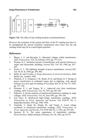


![Insulation Design 355
8.2 Field Computations
8.2.1 Analytical methods
For estimating electric stress levels at various critical electrodes, it is necessary
to find electrostatic field distribution. The field distribution can be determined
by a variety of methods. Classical methods such as the method of images give
accurate results whenever they can be applied. For complex configurations,
which exist inside a transformer, these methods cannot be applied. Initially,
transformer designers had to depend on analog methods in which conducting
paper and electrolytic tank analogs were used [1]. Before the advent of
computers and numerical methods, these methods were widely used for multi-
electrode and multidielectric material systems of transformers with two-
dimensional approximations of the problems. The stressed oil volume, required
for estimation of strength, was also calculated by direct plotting of equigradient
lines on a conducting paper analog by using suitable instrumentation [2]. Analog
methods are inconvenient, inaccurate, and expensive, and are limited in their
application. They may not be relevant now due to availability of advanced
computational techniques.
A conformal mapping technique such as the Schwarz-Christoffel
transformation has also been widely used for relatively simple geometries within
the transformers [3, 4]. In this method, the whole region of interest is mapped
into a new plane in which the solution is constructed involving unknown
constants in the transformation equation. The unknown constants are calculated
by solving a set of nonlinear equations which describe the boundaries of the
region in the original plane. Curved boundaries can also be handled in this
method. Although the method is suitable for regions with a single dielectric
material, for multidielectric problems an approximate solution can be obtained
by converting them into a single dielectric region by using equivalent insulation
distances. The method is best suited for a simply connected region containing
few electrodes. For multiple connected regions with complicated electrode
shapes and multiple dielectrics, this method is not suitable.
8.2.2 Numerical methods
In many cases, physical systems are so complex that analytical solutions are
difficult or impossible, and hence numerical methods are commonly used for
field computations. A numerical technique, the finite difference method (FDM),
is used in [5, 6]; it results in a set of linear equations which are solved by direct
matrix methods or iterative methods. FDM gives accurate results and can handle
curved boundaries accurately if more grid points are taken on the boundary. Its
main disadvantage is that the solution (potential distribution) is available at
discrete points only, and hence the method presents some difficulties where
quantities like stressed areas/volumes are required to be calculated [7].
www.EngineeringBooksPDF.com](https://image.slidesharecdn.com/transformer-engineering-design-technology-and-diagnostics-second-edition-pdf-230506172819-680afe24/85/transformer-engineering-design-technology-and-diagnostics-second-edition-pdf-pdf-376-320.jpg)
![356 Chapter 8
One of the most powerful and popular numerical techniques today is the
finite element method (FEM). It is in use for electrostatic field computations
since the last four decades [8]. Usefulness of the method has already been
demonstrated for magnetostatic and eddy current problems in earlier chapters.
At locations where the field is changing sharply, higher order polynomials can
be used to approximate the potential distribution within the corresponding
elements and/or a fine mesh can be used. As the method yields a set of linear
equations, solution can be obtained by direct matrix methods or iterative
methods. The electric stress in any element is calculated by differentiating the
approximated polynomial function. The stressed area between two equigradient
lines can be derived by finding the elements in which the stresses are within the
two limits of stress values.
Many adopt the charge simulation method (CSM) for electric field
computations because it is suitable for unbounded regions and it has high
accuracy [9]. In this method, physically distributed charges on the conductor
surface are replaced by discrete fictitious line charges placed outside the space
in which the field distribution has to be computed. The magnitudes of these
charges are calculated in order that their integrated effect satisfies the boundary
conditions exactly at some selected number of points on the boundary. The
method requires proper selection and placement of a large number of charges for
a reasonable accuracy. For example, a charge distribution on the surface of a
high voltage electrode can be replaced by k line charges placed inside the
electrode. For determining the magnitude of these charges, k points are chosen
on the surface of the electrode and the condition to be satisfied is as follows. At
each of these points on the electrode surface, the potential resulting from the
superposition of these fictitious charges should be equal to the conductor
electrode potential c
V ,
c
i
k
i
i V
Q
P ˜
¦
1
where i
P is a potential coefficient and i
Q is a discrete fictitious line charge.
When the above equation is applied to all the selected points k, we obtain a
system of k linear equations which are solved to obtain the magnitudes of the k
charges. The electric field value at any point in the domain then can be
determined easily by the superposition principle using these k charges.
CSM is not suitable for complex electrode configurations with multiple
dielectrics. On the contrary, FEM is most suitable for complex but bounded
problems. For electrodes with very small radius, because of the limitation on the
smallest size of the element that can be used and the approximation of a curved
path by small line segments, the accuracy of FEM may not be the best. Hence,
advantages of CSM and FEM can be combined with elimination of their
disadvantages in the combination method as reported in [10]. In this method, the
www.EngineeringBooksPDF.com](https://image.slidesharecdn.com/transformer-engineering-design-technology-and-diagnostics-second-edition-pdf-230506172819-680afe24/85/transformer-engineering-design-technology-and-diagnostics-second-edition-pdf-pdf-377-320.jpg)
![Insulation Design 357
entire problem space is divided into two parts; CSM is used mainly for the open
space with infinite boundary and FEM is used for the finite enclosed space.
8.3 Factors Affecting Insulation Strength
The breakdown voltage of a dielectric material is a statistically distributed
quantity and varies as a function of its physical/chemical properties and
impurities present in it. Failures may not always be initiated by high electrical
stresses; interrelated thermal, chemical and mechanical factors may have
significant influence on the breakdown processes. As compared to metals,
insulating materials exhibit an erratic behavior. With aging and/or deterioration
of electrical and mechanical properties, it becomes even more difficult to predict
their performance. In transformers, a composite oil-solid insulation system is
used. The erratic behavior of the oil is pronounced when used alone. There is a
much larger scatter of its breakdown voltage as compared to that of air. The
large scatter may be associated with random paths of streamers and variations in
their progress in the oil [11]. Hence, large oil ducts are always subdivided by
solid insulation into small ducts due to which the transformer insulation system
becomes more dependable and stable.
Compared to the breakdown processes in gases, the processes that initiate
and lead to breakdowns in the oil are difficult to comprehend. General models
using micro-bubble and weak-link theory have been attempted. It is reported in
the literature that some micro-bubbles exist in the oil even in the absence of an
electric field, and the application of a field creates additional bubbles. It is
suggested that discharges are ignited in these micro-bubbles. Due to
dielectrophoretic forces, particles/impurities are swept from surrounding oil
regions to the points of highest stress in the oil gap [12]; the corresponding
theory is described in the following subsection. These particles then tend to line
up along the electric field lines to create a weak-link in the oil gap; this
phenomenon is accentuated in the presence of moisture. Transformer designers
use to a great extent semi-empirical data for the insulation design as there is still
no coherent theory of oil breakdown.
8.3.1 Suspended solid particle mechanism
Transformer oil may contain some amount of solid impurities in the form of
fibers or dispersed particles [13]. Along with the solid impurities, bubbles
generated during overload periods are also present in the oil [14]. If each of
these impurities is considered as a sphere of radius r and permittivity H ,
immersed in oil having permittivity oil
H , then in an electric field E they are
polarized and have induced dipole moment in them. The force they experience is
given as [13, 15, 16]
www.EngineeringBooksPDF.com](https://image.slidesharecdn.com/transformer-engineering-design-technology-and-diagnostics-second-edition-pdf-230506172819-680afe24/85/transformer-engineering-design-technology-and-diagnostics-second-edition-pdf-pdf-378-320.jpg)
![358 Chapter 8
3
2
oil
oil
r
§ ·
H H
v ˜’
¨ ¸
H H
© ¹
F E E .
If E is only in the x-direction the above expression reduces to
3
3
3
2
2
.
2
oil
x x x y z x x
oil
oil
x x x
oil
oil x
x x
oil
r E E
x y z
r E E
x
E
r E
x
§ ·
½
H H w w w
v ˜
¨ ¸
® ¾
¨ ¸
H H w w w
¯ ¿
© ¹
§ ·
H H w
v ¨ ¸
H H w
© ¹
H H w
v
H H w
F a a a a a
a
a
. (8.12)
If oil
H ! H , which is true for solid particles or bubbles with water vapor content,
the force on the particles/bubbles is directed towards the high electric field
region according to Equation 8.12. If oil
H H , which is true for air bubbles
(without water content), the force on the bubbles is directed towards the low
electric field region. For metal particles H o f , therefore the quotient in the
above expression reduces to unity and the force on the metallic particles, which
is high in comparison to nonmetallic particles, is directed towards the high
electric field region.
8.3.2 Effect of moisture and impurities
Needless to say, moisture and other impurities have a significant deteriorating
effect on the dielectric strength of the transformer insulation. The moisture has a
deteriorating effect on both electrical and mechanical properties of the
insulation. As the moisture content in oil increases, strength reduces drastically
until the saturation point, after which there is no appreciable further
deterioration of the strength. Hence, percentage saturation is a decisive factor
influencing the dielectric strength of the transformer oil [17, 18]. The degrading
effect of the moisture is also significantly affected by the amount of other
impurities present in the oil [19]. The presence of solid impurities makes the
effect more significant even with low moisture content in the oil. The solid
insulation has more affinity (as compared to the oil) for moisture. It has been
reported in [20] that at room temperature, the reduction in the dielectric strength
of the oil due to cellulose particles becomes manifold at high moisture levels.
An increase in pressure or temperature increases the quantity of a gas the
oil can hold. If the oil temperature rises owing to an increase in ambient
temperature or load, the oil expands and the pressure increases. When the
pressure falls, the oil has more gas content than it can hold. The excess gas
content eventually diffuses out of the oil after some time (a few days or weeks)
depending on the ratio of the oil surface exposed to the gas and the total oil
www.EngineeringBooksPDF.com](https://image.slidesharecdn.com/transformer-engineering-design-technology-and-diagnostics-second-edition-pdf-230506172819-680afe24/85/transformer-engineering-design-technology-and-diagnostics-second-edition-pdf-pdf-379-320.jpg)
![Insulation Design 359
volume. If the pressure drops suddenly, gas bubbles may be formed in the oil,
reducing its dielectric strength [19].
The dielectric strength of paper insulation is largely decided by its
mechanical properties. A brittle paper having lost its mechanical strength has a
low dielectric strength. Aging of insulation affects its mechanical strength more
significantly than the electrical strength [19]. The rate of ageing increases
rapidly with an increase in temperature and the mechanical properties
deteriorate. An aged transformer may have 2% to 3% of moisture.
Many studies have been reported in the literature [17, 20–23] highlighting
the effects of various influencing factors, viz. temperature, pressure, impurities,
moisture, electrode shape/surface, electrode metal, applied voltage and its
duration, gap between electrodes, etc., on the oil breakdown strength.
The presence of moisture in the regions of high electric field regions may
lead to partial discharges [24]. Moisture may loosen the clamping system and
therefore reduce the ability of a transformer to withstand short-circuit forces.
The various sources of moisture in a transformer are (a) residual moisture
(typically 0.5% or less after factory processing), (b) ingressed moisture (during
repair/installation, due to poor sealing at joints, and due to a pressure difference
with respect to atmosphere), and (c) aging of cellulose insulation.
Under normal operating conditions, temperature variations in a
transformer are the major cause for the transfer of moisture between paper
insulation and oil. As the temperature increases, some amount of the moisture
present in the paper insulation transfers to the oil, and when the temperature
decreases, the moisture returns back, but at a slower rate, from the oil to the
paper. The distribution of water in the layers of paper insulation is nonuniform.
Water molecules migrate from hot inner layers closer to conductor surfaces to
outer colder layers [25].
Free water may appear in the transformer oil when moisture in it exceeds
the saturation value. This happens, for example, when a transformer is tripped
on a cool day after some time of operation at high temperatures. As the
temperature decreases abruptly, the water solubility in oil reduces quickly and
the moisture returns to the paper but this reverse process is slower as mentioned
earlier. Therefore, free water appears in the oil, which will reduce its dielectric
strength.
8.3.3 Effect of time and frequency
Volt-time characteristics are specific curves representing the relationship
between voltage and time-to-breakdown. These characteristics are generally
governed by the fact that some amount of energy is required to cause the
breakdown of a gap, and thus the breakdown voltage and the corresponding time
are interdependent [26]. The higher the voltage the lower the time is to cause the
breakdown. A typical volt-time curve of air insulation is shown in Figure 8.7.
www.EngineeringBooksPDF.com](https://image.slidesharecdn.com/transformer-engineering-design-technology-and-diagnostics-second-edition-pdf-230506172819-680afe24/85/transformer-engineering-design-technology-and-diagnostics-second-edition-pdf-pdf-380-320.jpg)
![360 Chapter 8
Voltage
Time
Figure 8.7 Typical volt-time curve.
In short-time power frequency overvoltage tests, the breakdown strength
of solid insulation is influenced by temperature. When an alternating voltage is
applied, initially the heat on account of dielectric losses is stored inside the
insulation, and its temperature begins to rise. The heat is dissipated to
surrounding ambient which is at a lower temperature. The insulation
temperature continues to rise until a state of equilibrium is reached, wherein the
heat dissipated is equal to the heat generated. But with an increase in the
temperature, the resistance of the solid insulation decreases due to its negative
temperature coefficient of resistance resulting in an increase of its leakage
current. Losses further increase due to the increased current value, and this leads
to a run-away condition resulting in an eventual breakdown. Hence, with an
increase in the time of application of the voltage, the dielectric strength reduces.
For most insulating materials, the infinite time strength is approximately two-
thirds of the one-minute strength, and the one-second strength is about 1.6 times
the one-minute strength [27].
The dependence of the oil dielectric strength on the duration of voltage
application is erratic as compared to the solid insulation. Although it is difficult
to obtain definite volt-time characteristics, it can be said that the dielectric
strength reduces rapidly after a few seconds and remains more or less constant
after a few minutes for power frequency test voltages. It requires time for
impurities to get lined up and bridge the gap; hence for a very short time period
of voltage application the strength is very high.
The frequency of the test voltage has a significant effect on the insulation
strength; its increase results in reduction of the strength, and thus increases
rapidly the severity of the power-frequency overvoltage test. As the frequency
increases, the dielectric loss and the heating effect increase, reducing the
strength of the solid insulation. The strength does not vary linearly with the
reciprocal of the frequency [28] but approximately with an exponent of 0.137,
i.e., strength .
)
1
( 137
.
0
f
v The frequency has a much smaller effect on the oil
strength compared to that on the solid insulation. In general, it can be concluded
that an increase in the frequency has a harmful effect on the strength of
www.EngineeringBooksPDF.com](https://image.slidesharecdn.com/transformer-engineering-design-technology-and-diagnostics-second-edition-pdf-230506172819-680afe24/85/transformer-engineering-design-technology-and-diagnostics-second-edition-pdf-pdf-381-320.jpg)
![Insulation Design 361
transformer insulation during the power-frequency overvoltage test. If the
frequency is increased, the time of application of the test voltage should be
reduced to produce the same amount of dielectric stress. Hence, standards
specify the total number of cycles for the power frequency induced overvoltage
test. When this test (in which the insulation is stressed to at least twice the
voltage/turn) is conducted, the frequency is also increased in order to avoid core
saturation. The IEC standard 60076-3, second edition: 2000, specifies that the
test time should be 60 seconds for any frequency up to and including twice the
rated frequency. For a test frequency higher than twice the rated frequency, the
test time should be reduced and calculated in accordance with the following
formula,
frequency
test
frequency
rated
duration
test u
120 seconds (8.13)
subject to a limit that it should not be less than 15 seconds. In other words, the
number of cycles for the test is fixed; 6000 cycles for 50 Hz and 7200 cycles for
60 Hz transformer. Hence, for a 50 Hz transformer, if the test is conducted at
200 Hz, the test duration should be 30 seconds.
The effect of the time of application and frequency of the voltage (during
power-frequency overvoltage tests) on the creepage strength is not significant as
compared to that on the puncture of solid insulation [28]. The creepage
breakdown in the absence of conducting material impurities is mostly decided
by oil failure, and an increase in the frequency does not result in significant
decrease of the oil strength due to a smaller heat effect [29].
Regarding impulse volt-time characteristics, two types of curves have
been derived in the literature. For the first one, called full-wave volt-time curve,
a full impulse wave is applied across the insulation and the breakdown may
occur either on the wave-front or wave-tail portions or it may not occur if the
voltage is low. A volt-time curve is plotted using these breakdown points. For
the second one, the wave-front slope is varied, and for each slope value the
voltage is increased till the breakdown occurs. This front-of-wave volt-time
curve is of similar nature but has somewhat different values as compared to the
full-wave volt-time curve.
The impulse volt-time curve of the insulation used in a transformer is
drastically different than that of air insulation. Typical curves for oil and oil-
impregnated pressboards are shown in Figure 8.8. The curves indicate that the
oil and solid insulations have flat characteristics after few microseconds.
Composite oil-solid insulation system generally has volt-time characteristics
close to that of the solid insulation alone. It is reported in [30] that the
dependence of dielectric strength on the impulse duration in the range of 10–3
to
10–1
seconds is small for major insulation consisting of oil-barrier system (e.g.,
gaps between windings).
www.EngineeringBooksPDF.com](https://image.slidesharecdn.com/transformer-engineering-design-technology-and-diagnostics-second-edition-pdf-230506172819-680afe24/85/transformer-engineering-design-technology-and-diagnostics-second-edition-pdf-pdf-382-320.jpg)
![362 Chapter 8
Time in microseconds
10 10 10 10 10
Voltage
4
3
1 2
0
(a)
3 4 5
10 10 10
10
0 1 2
Time in microseconds
10 10
Voltage
(b)
Figure 8.8 (a) Volt-time curve of oil-gap; (b) Volt-time curve of oil-
impregnated pressboard.
The impulse ratio can be defined as the ratio of the impulse full wave
strength to the one-minute r.m.s. AC (50 or 60 cycles) strength. Long ago,
researchers reported the impulse and one-minute volt-time characteristics [31,
32, 33] and the corresponding impulse ratios. Later, the volt-time curves for
partial discharge inception voltages have also been investigated. The partial
discharge and breakdown volt-time curves, and corresponding impulse ratios are
reported in [34] for three different configurations, viz. turn-to-turn insulation,
disk-to-disk insulation and oil gaps between barriers. It has been shown that the
breakdown volt-time curve, as expected, is significantly above the partial
discharge volt-time curve in the microsecond range. The two curves come very
close to each other in the AC long-term region of several minutes as shown by
the typical curves in Figure 8.9. It means that for very short times, a partial
discharge initiated is not sufficient, whereas in the longer duration of several
minutes its magnitude is sufficient to cause a breakdown.
During factory testing, different dielectric tests, lightning impulse,
switching impulse, and short-time/long-time power frequency tests, are carried
out separately independent of each other. In actual power system operation, the
www.EngineeringBooksPDF.com](https://image.slidesharecdn.com/transformer-engineering-design-technology-and-diagnostics-second-edition-pdf-230506172819-680afe24/85/transformer-engineering-design-technology-and-diagnostics-second-edition-pdf-pdf-383-320.jpg)
![Insulation Design 363
transformer may be subjected to superimposed AC and lightning impulse
voltages. The dielectric strength under such superimposed AC and lightning
stress levels is reported in [35]. The breakdown voltage under the superimposed
stress condition can be significantly lower than the corresponding value for the
lightning impulse alone.
Gas-insulated substations (GIS) are being used widely all over the world.
Disconnecting switch operations in GIS generate steep front transient
overvoltages characterized by a rise time of a few nanoseconds (5 to 20 ns), a
short duration of several microseconds, and amplitude as high as 2.5 per unit.
The 50% breakdown probability voltage of oil-paper insulation is reported to be
lower for steep-fronted GIS transients than for lightning impulses [36]. Oil-
paper insulated equipment like transformers or their bushings, when subjected to
GIS transients, may fail at voltages below the lightning impulse level. Hence,
the insulation of transformers for the GIS applications must be designed with
due consideration to these steep-fronted transients.
Sometimes transformers are subjected to high frequency oscillatory
overvoltages. In such cases, the damping of oscillations (defined as the ratio of
two consecutive amplitudes of same polarity) has significant impact on the
dielectric strength of their insulation; the strength increases with the increase in
damping. For example, the breakdown strength for an undamped oscillating
voltage having a frequency of 0.9 MHz is below the dielectric strength for the
lightning impulse voltage, whereas with a damping ratio of 0.9 the strength is in
the same range of as that for the lightning impulse voltage [37].
8.3.4 Effect of temperature
As temperature increases, the dielectric strength of most of the solid insulations
reduces. Due to an increase in the dielectric loss (and the power factor), the
temperature goes up further. The ohmic resistance of the insulation reduces with
increasing temperature, which results in flow of more current through it. It may
finally lead to a current run-away condition and an eventual breakdown.
10Ŧ6 10Ŧ4 10Ŧ2 100 102 104
Voltage
Time (Seconds)
PD
BD
Figure 8.9 Breakdown (BD) and partial discharge (PD) volt-time curves [34].
www.EngineeringBooksPDF.com](https://image.slidesharecdn.com/transformer-engineering-design-technology-and-diagnostics-second-edition-pdf-230506172819-680afe24/85/transformer-engineering-design-technology-and-diagnostics-second-edition-pdf-pdf-384-320.jpg)
![364 Chapter 8
The oil dielectric strength usually increases with temperature in the
operating range. A marked improvement in the strength is observed at high
temperatures for the oil containing high moisture content. The temperature
effects are dynamic in the sense that a considerable amount of time is required
for establishing equilibrium between moisture in the oil and that in the solid
insulation made from cellulose material. During different thermal loading
conditions, there is continuous interchange of moisture affecting the strength to
some extent. For a reasonable temperature rise, the amount of moisture in the oil
reduces, which helps to keep the transformer insulation system in a healthy
condition. It is known that an increase of temperature usually increases the
mobility of carriers and hence the conductivity. Hence, the breakdown voltage
of the oil should decrease with an increase in its temperature; experiments
conducted by many researchers show the opposite trend. Variations in the
mobility of carriers, therefore, may not possibly be used to explain the results of
experiments. There is some amount of gas bubbles present in the oil and their
solubility increases with temperature; this explains the increase of strength with
the temperature [38]. Hence, it is generally not preferable to keep a transformer
idle for a long time. Even a spare transformer should be kept in a no-load
condition for a reasonable amount of time periodically. The strength increases
with temperature from –5°C to about 80 to 100°C; above which it reduces [27,
39]. Below –5°C, the strength increases rapidly as moisture particles in the
suspension are frozen.
8.3.5 Effect of thickness
It is well-known that the dielectric strength of an insulating material does not
generally increase in direct proportion to its thickness in a nonuniform field
condition. The strength can be expressed in terms of the thickness by the
following simple exponential formula [40]:
n
thickness
E )
(
v . (8.14)
The numerical constant n varies from 0.5 to 1.0 depending on the
processing/treatment of the material and the degree of nonuniformity of the
field. For an untreated insulation, n is lower as compared to a treated insulation.
For better shaped electrodes giving uniform fields, its value is higher. For an
electrode with a small radius, there is more crowding of equipotential lines at its
surface resulting in a high stress and a low value of the breakdown voltage. The
above equation indicates that as the voltage rating increases, the insulation
content of the transformer increases more rapidly.
8.3.6 Stressed volume effects
The breakdown strength of the transformer oil decreases as its stressed volume
increases [41]. This is also in line with the general fact that the insulation
www.EngineeringBooksPDF.com](https://image.slidesharecdn.com/transformer-engineering-design-technology-and-diagnostics-second-edition-pdf-230506172819-680afe24/85/transformer-engineering-design-technology-and-diagnostics-second-edition-pdf-pdf-385-320.jpg)
![Insulation Design 365
strength reduces when its area under test increases [42]. The oil dielectric
strength reduces as its stressed volume increases for both power frequency and
impulse voltages [17]. Although, designers take either the stressed area or the
stressed volume for strength considerations, it is generally agreed that the size of
the structure is instrumental in the breakdown process. The strength calculations
based on the stressed oil volume are more commonly used in the industry. The
breakdown of a gap is usually initiated at the weakest spot under a high stress
condition. If in some other gap a greater volume of oil is subjected to the same
level of stress, it is quite probable that a still weaker spot is present, resulting in
the breakdown at a lower voltage. The amount of impurities and electrode
protrusions become important considerations for the area/volume effects.
Usually the relationship between the breakdown strength and the stressed
volume is obtained experimentally from many breakdown studies for various
types of electrode configurations. The breakdown strength for a plain oil gap is
expressed in terms of the stressed oil volume (for power frequency test voltages)
as [12]
137
.
0
9
.
17
SOV
E kVrms/mm (8.15)
where the stressed oil volume (SOV) is in cm3
. In [43], the 50% breakdown
probability stress for one-minute power frequency voltage is calculated as
5
2
5
11 5
9
1
.
SOV
.
E .
kVrms/mm (8.16)
where SOV is in cm3
. It can be verified that the strengths given by Equations
8.15 and 8.16 give the values of E of the same order for practical values of SOV
(e.g., in the case of a high voltage lead to ground configuration). The design
should be such that the calculated stress value should be lower than E by some
experience-based margin. It is assumed in the above equations that electrodes
are covered with some minimum thickness of paper insulation.
Thus, if a failure is predominantly decided by particles/impurities, a larger
oil volume will provide more particles which are drawn into high stress zones,
which may subsequently lead to a breakdown. However, a point is reached after
which a further increase in the volume will have an insignificant effect on the
strength since there is little influence of the field on remote zones unless the
field divergence is low. Hence, the volume in the above equations is taken as
corresponding to the region in which the calculated electric stress values are
between the maximum value and 90% of the maximum value.
Equations 8.15 and 8.16 tell us that as the stressed volume increases, the
dielectric strength of the insulation system reduces. If the electrode radius is
increased, the stress values reduce, but at the same time the stressed oil volume
increases reducing the withstand. Hence, an optimum electrode contour can be
determined by studying the relative variations in the stress and strength values
with different electrode contours [44].
www.EngineeringBooksPDF.com](https://image.slidesharecdn.com/transformer-engineering-design-technology-and-diagnostics-second-edition-pdf-230506172819-680afe24/85/transformer-engineering-design-technology-and-diagnostics-second-edition-pdf-pdf-386-320.jpg)
![366 Chapter 8
8.3.7 Creepage phenomenon
The solid insulation is used inside a transformer at many places, viz. between
turns, between layers, between disks, between a winding and ground, and
between windings. The designer is confronted with mainly two types of
electrical failures: puncture and creepage. The creepage strength of the solid
insulation is significantly lower than its puncture strength. Along equipotential
lines the creepage strength is maximum; therefore the electric field (E) should
be normal to the insulation surface (since the equipotential lines are at right
angles to the electric field). Due to complications of winding construction and
connections, it is difficult to keep the field normal to the insulation surface
everywhere. Also, it is not always possible to bend the solid insulation
components to any desired radius. In any case, considering the fact that the
electric field is actually a 3-D quantity, difficulties of having shaped insulation
components normal to the field are obvious. The places where there is a field
component parallel to the insulation surface, the strength is significantly
reduced. When there is a failure along the surface of insulation, it is termed a
creepage failure phenomenon. If the placement of the solid insulation results in
stresses along its surface, much of the purpose of using it, viz. subdivision of oil
ducts for higher overall strength, may be defeated.
The creepage flashover characteristics of oil-pressboard interfaces have
been analyzed and reported in the literature [45, 46]. A permittivity mismatch of
two insulation materials usually assists flashover phenomenon at their interface
[47]. The electric field in the oil immediately adjacent to the pressboard is
distorted due to the permittivity mismatch. Significant improvements can be
made by matching permittivities of the oil and pressboard insulations [48]. Thus,
a pressboard material having permittivity close to that of the oil not only reduces
the oil stress but also results in a higher value of the flashover voltage along the
oil-pressboard interfaces [49]. Hence, with a low permittivity pressboard, there
is significant scope for optimization of insulation content since the electric field
distribution will become more uniform in the oil-paper-pressboard insulation
system of transformers. A low permittivity pressboard, manufactured by
blending polymethylpentene fibers with cellulose fibers, has been used in a 765
kV, 500 MVA transformer [49].
1 2 3 4 5
-x 0 +x
64 kV 58 kV 50 kV 38 kV 35 kV
V1 V V V V
2 3 4 5
Figure 8.10 Cumulative stress calculation.
www.EngineeringBooksPDF.com](https://image.slidesharecdn.com/transformer-engineering-design-technology-and-diagnostics-second-edition-pdf-230506172819-680afe24/85/transformer-engineering-design-technology-and-diagnostics-second-edition-pdf-pdf-387-320.jpg)
![Insulation Design 367
8.3.8 Cumulative stress calculations
Using calculations based on SOV, the strength of an oil gap can be calculated as
discussed in Section 8.3.6; SOV-based calculations are more relevant for larger
oil gaps. Another approach, in which cumulative stress calculations are done, is
commonly used for the design of the insulation system of transformers. The
approach is used for both creepage withstand assessment and oil gap design.
For estimating creepage withstand characteristics, cumulative stress
distributions are determined along oil-solid interfaces. For a two-electrode case,
finding the cumulative stress distribution is easy. The maximum stress is usually
at one of the electrodes, and it reduces as we move toward the other electrode.
Hence, the cumulative stress at any point is the difference between the electrode
voltage and the voltage at that point divided by its distance from the electrode.
For complex electrode configurations, with more than two electrodes, the
maximum stress may not be at one of the extremities of the path (interface)
under consideration, in which case the cumulative stress calculation should be
started from the maximum stress point. The creepage stress distribution along a
solid-oil interface can be calculated by using the procedure described in [50].
Let us consider a solid-oil interface shown in Figure 8.10 and assume that
the potential values, calculated by some method at points 1, 2, 3, 4 and 5, spaced
at 2 mm distance, are as given in the figure. It is also assumed that the stress is
maximum at point 3 (7 kVrms/mm). The creepage stress is calculated for a unit
length of 2 mm in either direction from point 3, and the path is extended in the
direction of higher stress. Next, the cumulative stress is calculated for 4 mm
length in either direction as shown in Table 8.1. The calculation procedure is
continued till the entire path is traced. The calculated cumulative stress values
are plotted in Figure 8.11. The withstand for each of these creepage distances
(for power frequency overvoltages) can be calculated by [51]
37
.
0
2
15
d
Ecreep kVrms/mm (8.17)
Table 8.1 Cumulative Stress Calculation
Cumulative stress calculation
Path
length
(mm)
+ x direction í x direction Path extended
to point
2
kV/mm
0
.
6
2
4
3 V
V
kV/mm
0
.
4
2
3
2 V
V 4
4
kV/mm
75
.
3
4
5
3 V
V
kV/mm
0
.
5
4
4
2 V
V 2
6
kV/mm
83
.
3
6
5
2 V
V
kV/mm
33
.
4
6
4
1 V
V 1
www.EngineeringBooksPDF.com](https://image.slidesharecdn.com/transformer-engineering-design-technology-and-diagnostics-second-edition-pdf-230506172819-680afe24/85/transformer-engineering-design-technology-and-diagnostics-second-edition-pdf-pdf-388-320.jpg)
![368 Chapter 8
2 2.5 3 3.5 4 4.5 5 5.5 6
0
2
4
6
8
10
12
Path length in mm
Cumulative
stress
kV/mm
withstand curve
Figure 8.11 Plot of cumulative stress.
where d2 is the creepage path length in mm. The equation is valid for a degassed
oil and a good quality solid insulation with clean surface, and is in agreement
with the curve deduced in [52, 12] by considering creepage field strengths for
four different configurations.
It should be remembered that the calculated cumulative stress levels
should be lower than the value given by Equation 8.17 by a margin depending
on quality of components and manufacturing processes, i.e., the margin between
the creepage withstand and creepage stress for any length should be more than a
certain value fixed by the designer based on experience/established practices.
Usually, the creepage strength is considered about 30% lower than the bulk oil
(jump) strength [53, 54].
The reference withstand curve for bulk oil, subjected to power frequency
overvoltages, is described by the following equation [12],
38
0
1
18 .
oil d
E
kVrms/mm (8.18)
where d1 is the oil gap in mm between covered electrodes, and the oil is
considered without gases.
It is always advisable to cover the electrodes with some insulation as it
improves the strength by about 15 to 20% [12]. The creep withstand calculated
by Equation 8.17 is about 17 to 13% lower than the bulk oil withstand given by
Equation 8.18 (for a length of 1 to 100 mm), but as a conservative value it can
be taken 30% lower as mentioned earlier for any distance. The creep withstand
has been taken about 21% lower than the bulk oil strength in [55].
Thus, we have seen that there are two distinct approaches for determining
the withstand for bulk oil breakdown phenomena; one is based on the distance
www.EngineeringBooksPDF.com](https://image.slidesharecdn.com/transformer-engineering-design-technology-and-diagnostics-second-edition-pdf-230506172819-680afe24/85/transformer-engineering-design-technology-and-diagnostics-second-edition-pdf-pdf-389-320.jpg)
![Insulation Design 369
(Equation 8.18 above) and the other is based on the stressed oil volume
(Equation 8.15 or 8.16). These two approaches do not contradict each other, and
the consistency of the strengths obtained from the gap length and stressed oil
volume considerations has been elaborated in [12].
8.3.9 Effect of oil velocity
The velocity of oil has noticeable influence on its breakdown characteristics. It
is reported in [43] that the power frequency breakdown voltage of moving oil is
higher than that of stationary oil by 10 to 15% at about 5 cm/s, and it reduces
and becomes equal to that of the stationary oil at a velocity of about 25 cm/s. It
reduces further for higher velocities. The explanation for this particular behavior
is as follows. If oil movement is more dominant than the force by which
impurities are swept and drawn in high stress zones as observed in the case of
stationary oil, the breakdown voltage tends to be higher as the velocity
increases. When it increases beyond a certain value, reduction of the breakdown
voltage may be linked to the stressed oil volume effect, wherein the probability
of a large number of impurities passing through a high stress zone between the
electrodes increases. This phenomenon is in line with the weak-link theory; the
chances that weak-links of the oil (particles/impurity) may initiate a discharge
are higher due to the fact that a higher volume of the oil passes through a high-
stress zone [18]. Contrary to this theory, a higher velocity shortens the time for
which impurities will remain in the high stress zone, and the breakdown voltage
should increase as per volt-time characteristics. Hence, the breakdown voltage at
higher velocities will depend on which of the two effects, the volt-time effect or
the oil volume effect, is the deciding factor. For impulse conditions, the
breakdown voltage does not seem to be affected by the oil velocity.
8.3.10 Processing of insulation
Removal of moisture and impurities from insulation is one of the most important
manufacturing processes. Removing moisture from the oil is relatively simple,
which can be done by conventional methods of filtration or heat/vacuum cycles.
However, most of the moisture is in the solid insulation (it can be as high as
99%). Hence, a challenge is to make the solid insulation dry efficiently and
quickly.
With an increase in the size of transformers, the time taken for processing
of their insulation also increases. The time taken by a conventional hot air-
vacuum process is considerably higher for large transformers with high voltage
ratings. The conventional drying method may take more than 7 days for a 220
kV class transformer. The method consists of heating the assembly of the core
and windings in an air medium and applying vacuum for extracting moisture.
Moisture in an insulating material can be reduced by raising its temperature
and/or by reducing water vapor partial pressure, i.e., by applying vacuum. The
application of a vacuum speeds the moisture extraction process; heating alone
www.EngineeringBooksPDF.com](https://image.slidesharecdn.com/transformer-engineering-design-technology-and-diagnostics-second-edition-pdf-230506172819-680afe24/85/transformer-engineering-design-technology-and-diagnostics-second-edition-pdf-pdf-390-320.jpg)
![370 Chapter 8
takes more time to remove a given amount of moisture from the solid insulation.
Depending on the rating and voltage class of the transformer, several cycles of
alternate heating and vacuum are required until the transformer insulation is
dried. A moisture content of less than 0.5% is usually taken as the acceptance
criterion for ending the process.
Requirement of a faster and more efficient process along with the need for
better insulation performance resulted in the development and use of the
kerosene vapor phase drying (VPD) method [56]. It is a fast and efficient
method in which kerosene vapor at a high temperature is used as the heating
medium instead of hot air (used in the conventional method). A special grade of
kerosene, heated to about 130°C in an evaporator and converted into vapor form,
is injected into the autoclave or transformer tank housing the assembly of the
core and windings. As the process of heating is done under vacuum, the
moisture extraction starts during the heating period itself. When the insulation
reaches a certain desired temperature, a fine vacuum is applied to remove the
remaining moisture. In the VPD process, windings and insulation systems are
almost uniformly heated, whereas in the conventional process inner insulation
components may not be heated adequately. The total process time in the VPD
method is less than half of that for the conventional method in which, as heating
is done through the medium of air in presence of oxygen, the temperature is
limited to about 110°C. On the contrary, in the VPD process, the drying is done
in an oxygen-free atmosphere (virtually in vacuum), and hence there are no
harmful effects or loss of insulation life even at 130°C. Thus, uniform heating at
a higher temperature under vacuum results in faster removal of moisture. The
VPD process has another advantage that the vapor condensing on colder
winding and insulation parts washes out impurities. This aspect is particularly
useful when one wants to clean windings of transformers which come back to
factory for repair. With uniform heating of all insulation parts, shrinkage is
uniform. Furthermore, shrinkage is negligible during operation on site, ensuring
the mechanical integrity of windings.
Low frequency heating (LFH) method is also used for the drying purpose,
particularly for distribution and medium range power transformers. A low fre-
quency (few mHz) impedance voltage is applied to the HV winding with the LV
winding short-circuited, which results in uniform heating of the windings of the
transformer (since the eddy current loss in the winding conductors, a cause of
uneven temperature distribution, is almost zero). The windings are heated to
110°C and the moisture in the solid insulation is removed in less time as com-
pared to the conventional technique, consisting of hot oil circulation and vac-
uum cycles, in which the operating temperature is about 60 to 80°C. The re-
quired impedance voltage is also low due to a very low frequency of operation.
Generally, a current less than 50% of the rated value is required to reach a de-
sired winding temperature. Main advantages of the technique are reduction in
the process time, energy savings, and on-site applicability. At the site, after tak-
ing the (wet) transformer out of service and with its oil removed, the method can
www.EngineeringBooksPDF.com](https://image.slidesharecdn.com/transformer-engineering-design-technology-and-diagnostics-second-edition-pdf-230506172819-680afe24/85/transformer-engineering-design-technology-and-diagnostics-second-edition-pdf-pdf-391-320.jpg)

![372 Chapter 8
time needs to be provided before the commencement of high voltage tests.
During the settling period, heavier particles/impurities settle down at the bottom
and the air bubbles move up or get absorbed. After the hold time, air bubbles
should be released by bleeding (through air release plugs) at the top so that the
transformer is free of (trapped) air. With this, dielectrically critical areas are
cleared. The hold time increases with the voltage rating of transformers. For 132
kV class transformers it should be minimum 24 to 36 hours, for 220 kV class it
should be about 48 hours, and for 400-500 kV class transformers it is desirable
to have the hold time of about 72 hours [57]. A lower hold time may be adopted
by the transformer manufacturers based on their experience.
8.4 Test Methods and Design Insulation Level (DIL)
In service, the transformer insulation is subjected continuously to operating
voltages and occasionally to overvoltages. The operating voltages decide the
working voltage stress on the insulation. The overvoltages can be broadly
divided into lightning overvoltages (aperiodic surges with duration of one to tens
of microseconds), switching overvoltages (oscillatory surges with duration up to
thousands of microseconds), and temporary overvoltages (lasting for few
minutes) at or close to the power frequency. Standards on transformers have
defined test levels for various voltage classes. There are basically four different
types of tests: a lightning impulse test, a switching impulse test, a short duration
power frequency test, and a long duration power frequency test with partial
discharge measurement. While the first three tests check the insulation’s
overvoltage withstand capability, the long duration test is mainly intended for
checking the insulation behavior under working voltage stresses. The design of
insulation between various electrodes is decided by one or more of these test
levels. An interdisk spacing is decided by impulse stresses, whereas the end
insulation between the windings and the top/bottom yoke is predominantly
decided by the power frequency test voltages. The conductor insulation is
decided by either the impulse stress or the working voltage stress.
When oil and solid insulation are stressed together, two kinds of failures
can usually occur. In one type, there could be a complete catastrophic failure
between two electrodes (e.g., jump breakdown, creepage breakdown or
combination of both). This kind of failure is uncommon if adequate clearances
are provided and maintained. The second one is a local oil failure (partial
discharge). In earlier days, the partial discharge (PD) measurement test was not
conducted due to nonavailability of proper instrumentation. Also, many partial
discharges used to result in undetected damages (since the solid insulation acted
as a barrier to propagation of discharges). With the development of
instrumentation and awareness of slow but damaging effects of discharges, the
partial discharge test has become one of the most important tests for high
voltage transformers. The international standards on transformers have defined
PD limits. Some manufacturers set their internal norms much lower than those
www.EngineeringBooksPDF.com](https://image.slidesharecdn.com/transformer-engineering-design-technology-and-diagnostics-second-edition-pdf-230506172819-680afe24/85/transformer-engineering-design-technology-and-diagnostics-second-edition-pdf-pdf-393-320.jpg)
![Insulation Design 373
specified in the standards in order to ensure long-term reliability of transformers.
In order to obtain very low PD levels, sharp electrodes inside the transformer
have to be rounded or electrostatically shielded. Processing and impregnation
procedures have to be excellent for minimizing impurities and air voids. Also,
the manufacturers should have proper instrumentation for the measurement of
low PD levels. Ambient partial discharges in the test area and surrounding
environment have to be minimized. Partial discharges lead to progressive
damage of insulation resulting in an eventual failure after a time period which
depends on their severity and location inside the transformer. Hence, it is
advisable to eliminate sources and causes of partial discharges so that
progressive deterioration of insulation becomes a remote possibility.
A transformer should be designed and manufactured such that it is partial
discharge free. It should be noted that the impregnation of insulation may not be
perfect and also it may not be possible to control the dielectric field uniformly at
all locations. Hence, in practice some amounts of partial discharges are always
there; efforts should be made to minimize them. Electric stress values below PD
inception levels do not result in aging of the mechanical strength of the
pressboard. In such a case, the life of the pressboard insulation is decided by the
mechanical strength as affected by thermal conditions [49]. PD is usually
measured either in pico-coulombs or micro-volts. Its detection and measurement
of PD is difficult. Methods for locating PD sources are discussed in Section
14.3.
Design insulation level: After calculating voltages at critical locations inside a
transformer (within the windings, at the ends of the windings, on the surface of
leads, etc.) under all test conditions, it is quite meaningful to convert these
voltages to one equivalent voltage, which is usually the one-minute short
duration power frequency voltage. This equivalent voltage level is called the
design insulation level (DIL) which is expressed in kVrms. Thus, at any point
inside the transformer, there is only one DIL, which is the maximum of the
equivalent one-minute power frequency voltage levels during the four different
tests. This approach is widely followed by transformer designers for simplifying
the insulation design process. The conversion factors used by different
manufacturers for converting the calculated voltages (under various tests) to the
one-minute r.m.s. level may not be identical but they fall in a narrow range. The
factors reported in [54] are given in Table 8.2.
Table 8.2 Factors for Conversion to One-Minute (r.m.s.) Power Frequency
Level
Test voltage Multiplication factor
Lightning Impulse Level (BIL) ~ (1/2.30)=0.44
Switching Impulse Level (SIL) ~ (1/1.80)=0.55
Long duration (one hour) power frequency voltage ~ (1/0.80)=1.25
www.EngineeringBooksPDF.com](https://image.slidesharecdn.com/transformer-engineering-design-technology-and-diagnostics-second-edition-pdf-230506172819-680afe24/85/transformer-engineering-design-technology-and-diagnostics-second-edition-pdf-pdf-394-320.jpg)
![374 Chapter 8
The conversion factor for the one-hour power frequency test voltage is in
agreement with the following equation given in [43],
0 055
1
1
.
t
V t V (8.19)
where 1
V and t
V are the 50% breakdown probability voltages for 1 minute and t
minutes, respectively. The equation gives 1
60 V
V as 0.8, which is in line with
that given in Table 8.2.
The multiplication factor for BIL in Table 8.2 is in accordance with the
impulse ratio (the ratio of the lightning impulse level to the power frequency
level) of about 2.3, as evident from Table 8.3 which gives commonly used BIL
and power frequency test levels for various voltage classes. An impulse ratio in
the range of 2.3 to 2.5 is being used in the industry [11, 12] while calculating the
equivalent DIL of a BIL value. This range of the impulse ratio represents an
average conversion factor for the impulse voltage duration in the range of 10 to
100 microseconds. The overvoltages stressing the interdisk or interturn
insulations during the impulse test may be shorter than 10 microseconds in
which case the conversion factor seems conservative. The impulse ratio of 2.68
has been suggested in [30] for 1.5/40 microsecond impulse waveform while
designing interwinding and interdisk insulations, giving the corresponding
multiplication factor of 0.37 for BIL in Table 8.2 (in place of 0.44). A lower
value may open avenues for insulation optimization since in that case the
equivalent DIL value is lower. On the other hand for impulse overvoltages of
more than hundreds of microseconds duration (close to switching transients),
there is a risk in using the impulse ratio between 2.3 to 2.5 and therefore it
should be lower. Thus, the conversion factor should be judiciously selected
based on detailed analysis and experimental data. For AC voltages and non-
oscillatory impulses having durations other than that of lightning, switching and
long duration power frequency voltages, an interpolation is done with caution
for finding DIL [53].
Having estimated the DIL at critical electrodes inside a transformer, one
can proceed with the design of its insulation system.
Table 8.3 Impulse Ratios
Voltage class BIL (kVp) Power frequency test level (kVrms) Impulse ratio
132 kV 550 230 2.39
220 kV 950 395 2.40
400 kV 1300 570 2.28
www.EngineeringBooksPDF.com](https://image.slidesharecdn.com/transformer-engineering-design-technology-and-diagnostics-second-edition-pdf-230506172819-680afe24/85/transformer-engineering-design-technology-and-diagnostics-second-edition-pdf-pdf-395-320.jpg)
![Insulation Design 375
LV HV
barriers
Insulating
Figure 8.12 Subdivided duct between LV and HV windings.
8.5 Insulation between Two Windings
The gap between the low voltage (LV) and high voltage (HV) windings is
subdivided into many oil ducts by means of solid insulating barriers (Figure
8.12). The insulation system of oil-cooled power transformers consists of a
combination of oil and solid insulation (paper and precompressed board). Both
of them are cheaper than most other insulating materials, and together they give
much higher dielectric strength than individually.
In an oil-pressboard insulation system, since the maximum admissible
stress in a good quality pressboard material for one-minute power frequency
overvoltage is about 40 kVrms/mm [53], the limiting design stress values are
primarily due to stress levels in the oil. In degassed oil with almost uniform field
distribution (e.g., between barriers in the HV-LV gap), a typical PD inception
field stress value for an 8 mm oil duct is 10 kVrms/mm for insulated winding
conductors [52, 58]. Since the stress is high at winding conductor corners, the
PD inception stress value for an 8 mm oil duct next to windings for degassed oil
is lower, i.e., about 8.4 kVrms/mm. The allowed (design) stress values can be
lower than these PD inception stress values depending on the required safety
margin and the quality of manufacturing processes. Thus, the dielectric strength
of the solid insulation is much higher than that of the oil. Since electric stress (E)
is inversely proportional to permittivity, the oil stress is significantly higher than
that in the solid insulation. The oil permittivity ( # 2.2) is about half that of the
solid insulation, hence the oil stress is twice the solid insulation stress in uniform
fields. Since the oil has to bear a higher stress, it is recommended to make
barriers as thin as possible and give more space for the oil ducts. In the oil-
paper-pressboard insulation system, the strength of the insulation arrangement is
predominantly decided by the strength of the oil ducts. Hence, the design of a
transformer insulation system essentially means proper dimensioning of oil
www.EngineeringBooksPDF.com](https://image.slidesharecdn.com/transformer-engineering-design-technology-and-diagnostics-second-edition-pdf-230506172819-680afe24/85/transformer-engineering-design-technology-and-diagnostics-second-edition-pdf-pdf-396-320.jpg)
![376 Chapter 8
ducts and oil-solid interfaces. For a given total gap between two windings, there
is no advantage gained by increasing the solid insulation thickness just because
its strength is higher. On the contrary, a high solid insulation thickness results in
more stress in oil ducts. The barriers should be as thin as possible, if permitted
from mechanical strength considerations. Barriers with a thickness of 1.5 to 2
mm are generally used for getting good mechanical stability. The lower the oil
duct width, the higher the withstand stress (kV/mm) is. The number of barriers
in an interwinding gap should be adequate so that larger oil gaps are avoided (oil
gaps larger than 14 mm are usually not recommended in the interwinding gaps).
Insulating barriers have an additional function of acting as barriers against the
propagation of a discharge streamer in the oil between electrodes. The barriers
break the oil path into smaller ducts and prevent the lining up of impurities in
the oil.
The size of the first duct next to windings should be properly chosen.
Although a small width is desirable as it gives higher kV/mm withstand value,
thermal considerations may not allow the use of duct width below 6 mm. The
first duct is usually of 6 to 10 mm size. Withstand for the ducts (the first duct
and the other ducts in the HV-LV gap) can be determined by referring to
published curves [52, 58] for four types of gaps, degassed oil between barriers,
gas saturated oil between barriers, a degassed first oil duct, and a gas-saturated
first oil duct. The maximum stress in the first duct has to be accurately
determined (say, by FEM). Breakdown gradients obtained for a typical
configuration are given in [30]. The values of breakdown gradients for a yoke-
end-line-lead arrangement (the line terminal at the yoke end of a winding) are
lower than those for a centerline-lead arrangement (the line terminal taken at the
midpoint of the winding stack with two parallel branches). This is because the
field distribution in the first duct at the line terminal is more nonuniform for the
former as compared to the latter arrangement. Actual design values should be
lower than the breakdown values depending on the margin to be kept. The HV-
LV (HILO) gap value is usually based on the average stress expressed as [59],
)
5
.
0
( insulation
solid
gap
HILO
DIL
Eav
u
. (8.20)
It typically has a value of about 6 kVrms/mm. A manufacturing tolerance is
added to the HILO gap calculated by the above expression. For a winding-to-
end-limb clearance (e.g., in a single-phase three-limb construction) or an
innermost-winding-to-core clearance, a lower value of Eav is used due to the
presence of sharp corners of the core. In some critical cases, an electrostatic
shield is used around the core/end limb facing the windings. The phase-to-phase
insulation design is very similar but the stresses due to switching impulse and
power frequency test levels need to be considered; most of the time the voltages
between phases are 150% of phase-to-ground voltage levels.
www.EngineeringBooksPDF.com](https://image.slidesharecdn.com/transformer-engineering-design-technology-and-diagnostics-second-edition-pdf-230506172819-680afe24/85/transformer-engineering-design-technology-and-diagnostics-second-edition-pdf-pdf-397-320.jpg)


![Insulation Design 379
Angle caps are used to protect the winding corners from another winding
or an end limb as shown in Figure 8.15. Angle rings/caps made from molded
material are usually available in a sector form, which have to be overlapped by
doing proper chamfering. The overlapping distance is usually kept as 30 to 40
times the thickness of the angle rings/caps.
Although it is essential to achieve near-uniform initial impulse voltage
distribution, what is more important from the insulation design point of view is
obtaining uniform dielectric stresses in relation to corresponding strength values.
Generally, it is very difficult to obtain equal initial impulse voltages between
disks/turns throughout the winding; the insulation should be designed such that
the margin between the strength and the stress is in the same range of values
along the winding height. This is an ideal design which may not be possible
since, for cooling purposes, adequate interdisk or interturn gaps are kept at the
neutral end even though the stresses are low. It is not advisable to increase the
turn or disk insulation, where stresses are high, without detailed calculations.
There could be failure even if extra insulation is provided because the increase
in the strength may not be commensurate with the increase in the stress due to a
reduced series capacitance value.
8.7 Design of End Insulation
In the composite oil-solid insulation system, the strength of an insulation
arrangement is predominantly determined by the strength of oil gaps. The solid
insulation is used to subdivide long oil gaps (having lower dielectric strengths)
into smaller ones. While assessing the end insulation design, the strengths of oil
gaps and solid-oil interfaces are evaluated. FEM is commonly used for
estimation of electrostatic field distribution. A typical end insulation
arrangement is shown in Figure 8.16. The electric stress distributions along
various contours between the windings and between the yokes and the windings
are examined [60]. Two such contours are shown in the figure by dotted lines.
For each oil duct within a selected contour (e.g., A-C), the cumulative
field distribution is determined by integrating the field along the contour starting
from the maximum value as described in Section 8.3.8. If in an oil gap, the
maximum stress is at one of the extreme ends, the calculations are greatly
simplified since the cumulative stress at any point with a distance of d from the
point of maximum stress on the contour is calculated as the voltage difference
between the two points divided by d. In this case the cumulative stress is
³
d
x
d dx
E
d
E
0
)
(
)
(
1
. (8.22)
The cumulative oil stress values for each oil gap along the contour A-C are
plotted and compared with a reference strength/withstand curve, described by a
formula such as Equation 8.18, as shown in Figure 8.17.
www.EngineeringBooksPDF.com](https://image.slidesharecdn.com/transformer-engineering-design-technology-and-diagnostics-second-edition-pdf-230506172819-680afe24/85/transformer-engineering-design-technology-and-diagnostics-second-edition-pdf-pdf-400-320.jpg)

![Insulation Design 381
The minimum safety margin is a function of quality of insulation and technology
of drying/oil impregnation processes. Usually a safety margin of 25 to 35% in
critically stressed parts of the transformer insulation is considered as sufficient
to pass successfully the long duration (one hour) induced overvoltage test
without partial discharges and also the impulse test [61].
The placement of angle rings/caps is an important aspect of the end
insulation design. They divide larger oil ducts into smaller ones increasing the
withstand of the total gap and the resulting oil ducts. The angle rings/caps
should be placed along the equipotential lines; otherwise higher creepage
stresses along their surface may reduce the overall dielectric strength. As we go
away from the winding corner, the radius of an angle ring/cap should be more so
that it lies along an equipotential line and the creepage stress on its surface is
minimized. The angle rings/caps with a fixed and small radius of 2 to 3 mm are
cheaper than the contoured ones with a much higher radius. However, the
creepage stress on the noncontoured angle rings/caps can be high, reducing the
overall strength of the insulation arrangement. In order to optimize end
insulation clearances, contoured angle rings/caps need to be used which reduce
not only the creepage stresses but also the oil duct sizes in high stress zones
thereby improving their withstand. The effectiveness of a contoured angle ring
can be clearly seen from Figure 8.18. The creepage stress along the portion AB
of the contoured angle ring is much less than that along the corresponding
portion CD of the noncontoured angle ring. The first angle ring/cap should be
close to the winding for having a smaller first oil duct width.
Apart from an effective subdivision of oil ducts by barriers/angle rings
(caps)/solid washers, it is necessary to reduce electric stresses at winding
corners. The stress can be reduced by placing a static end ring (SER) at the end
of the winding (see Section 7.3.4 for a discussion on SERs). The inner and outer
diameters of the SER have to be flush with the corresponding diameters of the
winding, and it should be as close to the winding end disk/turn as possible all
along the circumference.
(a) Contoured angle ring (b) Noncontoured angle ring
Figure 8.18 Effectiveness of contoured angle ring.
www.EngineeringBooksPDF.com](https://image.slidesharecdn.com/transformer-engineering-design-technology-and-diagnostics-second-edition-pdf-230506172819-680afe24/85/transformer-engineering-design-technology-and-diagnostics-second-edition-pdf-pdf-402-320.jpg)
![382 Chapter 8
R =2
2
6
R =
1
6
R =
1
paper insulation
SER
SER
R =2
2
Figure 8.19 Static end ring.
In low voltage windings, if the SER is dispensed with, a turn or disk angle
ring/cap is usually placed on the last turn/disk, which reduces the stress in the oil
duct immediately next to it.
A typical sketch of an SER is shown in Figure 8.19. The inner radius (R2)
close to the winding disk is usually standardized to 2 mm, whereas the outer
radius (R1) can be at least 6 mm and it may be more as the voltage rating and
radial depth of the winding increases. The paper insulation thickness is of the
order of 3 mm. A static ring (SR) may be placed between two disks of a
winding, particularly between the second and third disks and between the fourth
and fifth disks from the line end of a continuous disk winding since the lightning
impulse voltage appearing across these disks can be high.
Sometimes, the LV winding height is kept greater (by a few mm) than the
HV winding height. The stress at the LV corner facing the HV winding is lower
in this case compared to the case wherein the LV winding height is equal to or
shorter than the HV winding height.
8.8 High Voltage Lead Clearances
In high voltage transformers, the clearances between leads and ground, between
leads, etc. have to be judiciously selected. Consider a high voltage insulated lead
near a ground plane as shown in Figure 8.20. The maximum electric stress in the
paper insulation and the oil can be calculated by the well-known formulae given
in Section 8.1. The complete stress distribution can be accurately analyzed by
using FEM.
The oil duct strength can be computed on the basis of the stressed oil
volume (SOV) theory. The stressed volume between the maximum stress and
the contour of 90% of the maximum stress for a cylindrical lead-plane
configuration can be calculated by the following approximate formula [62],
www.EngineeringBooksPDF.com](https://image.slidesharecdn.com/transformer-engineering-design-technology-and-diagnostics-second-edition-pdf-230506172819-680afe24/85/transformer-engineering-design-technology-and-diagnostics-second-edition-pdf-pdf-403-320.jpg)
![Insulation Design 383
Lead
Paper insulation
Oil
Figure 8.20 High voltage lead insulation.
l
r
SOV
18
2
S
(8.23)
where r is the bare lead radius and l is the effective lead length. A more accurate
formula for a bare lead is given in [63]. SOV for a covered lead and/or for a
complex configuration of electrodes can be calculated by using FEM. The 50%
breakdown probability stress for one-minute power frequency voltage can be
calculated from the SOV value through Equation 8.16. The safe withstand value
is lower than this breakdown stress value and can be decided by the transformer
manufacturer depending on the acceptable value of the percentage breakdown
probability and the quality of manufacturing processes (which decide the level
of impurities) [43, 64]. The margin kept is also a function of manufacturing
practices and required working tolerances. For example, a lead-to-tank clearance
may actually be less than that specified in the drawing. Mechanical tolerances,
lowering clearances and magnetic clearances may dominate over the dielectric
design considerations in lower voltage ratings.
An increase in breakdown voltage for a lead-to-ground configuration can
be obtained by one or more of the following means: an increase in the clearance,
an increase of the bare lead diameter, an increase in the thickness of the paper
insulation, and placement of barriers to subdivide the oil duct. The first option is
obviously not cost effective as it increases the material cost and the size of the
transformer. Out of the remaining three options, the paper covering has
significantly more impact in improving the withstand [65]. With an increase in
the paper insulation, more voltage is dropped across it, reducing the stress in the
oil. Thermal considerations and manufacturing time are also the deciding factors
while standardizing the bare diameter, the paper insulation thickness, and the
clearance for various DILs. When the electrode is not sharp, barriers can be put
along equipotential lines to enhance the strength.
www.EngineeringBooksPDF.com](https://image.slidesharecdn.com/transformer-engineering-design-technology-and-diagnostics-second-edition-pdf-230506172819-680afe24/85/transformer-engineering-design-technology-and-diagnostics-second-edition-pdf-pdf-404-320.jpg)
![384 Chapter 8
It should be noted that the increase of either the bare lead diameter or the
paper thickness increases SOV, but the reduction in strength due to an increased
SOV is not significant as compared to the reduction in the stress value because
of the logarithmic relationship between the strength and SOV.
When there is a row of tap leads facing a winding or a tank wall, the
maximum stress is less compared to that in an isolated lead case. The extent of
the stress reduction has to be assessed for the worst configuration (giving
minimum reduction) and then the electrical clearances can be standardized
accordingly using the isolated lead-to-ground clearances. The clearance of the
row of tap leads to ground is usually lower as compared to that of the isolated
lead to ground case.
The above analysis has assumed a smooth ground plane. When the ground
electrode is not smooth and is having sharp corners, it becomes difficult to
standardize the clearances. It is preferable to have at least 2 mm radius at the
corners. With this minimum corner radius, in the absence of detailed analysis, 1
mm of oil gap per kVrms of the DIL seems to be a safe design criterion (i.e., an
average stress of 1 kVrms/mm). A value of about 1.4 kVrms/mm or more can be
used, based on experience.
In some cases due to nearness of high voltage electrodes to the tank, the
electric field at its surface may be high and therefore the tank surface should be
covered with proper insulation [53].
The above analysis holds good for jump clearances in oil between a lead
and ground. There is one more design consideration when leads are supported
by a solid insulation piece fixed to a grounded part as shown in Figure 8.21
(equipotential lines obtained from an FEM analysis are also displayed). In this
case, the cumulative creepage stress on the pressboard surface and the
corresponding withstand are calculated using the procedure given in Section
8.3.8. For nonhomogeneous field distributions (involving sharp electrodes), the
rule of 1 mm of creepage path per kVrms may be followed in the absence of
detailed analysis.
Sometimes insulating barriers are placed close to high voltage leads in
high stress zones. The combined effects of the oil velocity and particles
sweeping towards high stress zones, as discussed in Section 8.3.9, have a
definite role to play in power frequency breakdowns. The barriers make the oil
flow restricted in the high stress zones so that the probability of the occurrence
of breakdown phenomena (in which floating particles are drawn into high stress
zones helping breakdown processes) is reduced to a great extent. Hence, the
barriers can be quite effective when used to subdivide large oil gaps in the high
stress zones. They should be placed close to the electrode along equipotential
lines. If there is an appreciable creepage stress along their surface (due to
improper placement), the overall strength may not improve.
www.EngineeringBooksPDF.com](https://image.slidesharecdn.com/transformer-engineering-design-technology-and-diagnostics-second-edition-pdf-230506172819-680afe24/85/transformer-engineering-design-technology-and-diagnostics-second-edition-pdf-pdf-405-320.jpg)
![Insulation Design 385
Figure 8.21 Optimum creepage distance calculation by FEM analysis.
Nonuniform field patterns exist in the vicinity of high voltage leads
between winding terminations and lower bushing connections. Covering the
leads with thick paper insulation may not help much as the stress in the oil may
not be reduced significantly. Also, too much insulation on the leads limits their
thermal capability. The scatter of the breakdown voltage for such a wide oil duct
can be much higher resulting in lower dielectric strength. The modern lead exit
systems [54] consist of pressboard barrier systems which divide the oil gap into
smaller gaps. The lead is covered by a thin layer of molded pressboard.
8.9 Statistical Analysis for Optimization and Quality
Enhancement
8.9.1 Parameter design
Optimization of an insulation system requires identification of factors having
significant influence on stresses and strengths. Orthogonal array design of
experiments is a technique that allows the effect of several parameters to be
determined efficiently. The analysis of relative effects of the different factors
can be done by decomposition of variance which is commonly called as analysis
of variance (ANOVA).
An approach for the optimization of major insulation of a 400 kV class of
transformer has been described in [66]. Figure 8.22 shows a sectional view of
transformer windings, in which the insulation arrangement of two disks of its
HV winding is depicted. The factors affecting maximum oil stress and strength
are viz. the conductor radius (R), the conductor paper covering (PC), the disk
angle ring thickness (DAR), the HV-LV gap, the duct width between the disks,
www.EngineeringBooksPDF.com](https://image.slidesharecdn.com/transformer-engineering-design-technology-and-diagnostics-second-edition-pdf-230506172819-680afe24/85/transformer-engineering-design-technology-and-diagnostics-second-edition-pdf-pdf-406-320.jpg)
![386 Chapter 8
the first oil duct width and the voltage difference between the disks. The
quantification of the effect of these factors has been reported in [66], which is
based on 36 FEM simulations for specific combinations of the above seven
factors. Such an analysis helps designer to do parameter design, i.e., choosing
an optimum combination of the factors. A quadratic surface is generated by
using multiple regression analysis to express the oil stress in terms of the factors,
which has been used further for the tolerance design as explained below.
8.9.2 Tolerance design
Insulation optimization cannot be done in isolation without due consideration to
variations usually observed during the manufacturing processes. The tolerance
design methodology can be used to identify critical insulation components
whose manufacturing variation needs to be controlled. For this, the deviations in
dimensions of all (control) factors are first determined by choosing random
samples from the manufacturing site. The standard deviation ( SD ) can be
calculated from the data. For the tolerance design, three levels of the factors can
be taken around the mean ( m ) as SD
m 2
3
, m , and 3 2
m SD
[67].
Either FEM simulations can be used to obtain the oil stress values for the
specific combinations of the factors or the quadratic surface generated earlier (at
the parameter design stage) can be used expediting the analysis. The subsequent
ANOVA analysis can reveal the relative effects of manufacturing variations in
the factors on the stress values. This can help in identifying manufacturing
processes that need to be controlled on priority to help reliability
enhancement/optimization efforts. The extra investment needed to improve a
particular process can also be justified by such analysis.
duct between
first duct
arrangement
LVŦHV
gap
R
PC
HV winding
PC
angle
ring
disk 1 disk 2
disks
oil duct and barrier
Figure 8.22 Insulation arrangement between two disks.
www.EngineeringBooksPDF.com](https://image.slidesharecdn.com/transformer-engineering-design-technology-and-diagnostics-second-edition-pdf-230506172819-680afe24/85/transformer-engineering-design-technology-and-diagnostics-second-edition-pdf-pdf-407-320.jpg)


![ª º
393
9
Cooling Systems
The magnetic circuit and windings are the principal sources of losses and
resulting temperatures in various parts of a transformer. The losses in the core
and the windings, and the stray losses due to leakage and high current fields, are
mainly responsible for heat generation within the transformer. Sometimes loose
electrical connections inside the transformer, leading to a high contact
resistance, cause higher temperatures. Excessive temperatures due to heating of
curb bolts, that are in the path of a stray field, can damage gaskets (refer to
Chapter 5). The heat generated due to all these losses must be dissipated without
allowing the core, winding, and structural parts of the transformer to reach
temperatures that will cause deterioration of its insulation. If the insulation is
subjected to temperatures higher than the allowed values for a long time, it
looses insulating properties; in other words, the insulation is aged, severely
affecting the transformer life. There are two principle characteristics of the
insulation, viz. the dielectric strength and the mechanical strength. The dielectric
strength remains high up to a certain temperature after which it drops rapidly. At
this point the insulation material becomes brittle and loses its mechanical
strength. Thus, it is primarily the mechanical strength that is affected by higher
temperatures and aging, which in turn affects the dielectric strength. Hence, the
dielectric strength alone cannot always be depended upon for judging the effect
of temperature on the insulation [1].
Accurate estimation of temperatures on all surfaces is very critical in the
design of transformers to decide the operating flux density in the core and the
current densities in the windings/connections. It helps in checking the adequacy
of cooling arrangements provided for the active parts and in ensuring reliable
www.EngineeringBooksPDF.com](https://image.slidesharecdn.com/transformer-engineering-design-technology-and-diagnostics-second-edition-pdf-230506172819-680afe24/85/transformer-engineering-design-technology-and-diagnostics-second-edition-pdf-pdf-414-320.jpg)

![Cooling Systems 395
insulated conductors is exposed to the cooling medium, and the heat flows
through a small thickness of the conductor insulation. But in small transformers
the heat may have to flow through several layers of conductors and insulation
materials before reaching the cooling medium.
The temperature drop across the insulation due to the conduction heat
transfer mechanism can be calculated by the following basic thermal law:
T
Q R
T
' u (9.1)
where Q is the heat flow (power loss) in W, and T
R is thermal resistance in
°C/W. 2 1
T T
T
' , where 1
T is the temperature of oil and 2
T is the temperature
of the winding conductor. The thermal resistance is given by
i
T
t
R
k A
u
(9.2)
where i
t is the insulation thickness in m, A is the cross-sectional area in m2
, and
k is the thermal conductivity in W/(m °C). If q denotes heat flux per unit
transfer area, the temperature drop across the insulation can be rewritten as
i
q t
k
T
u
' . (9.3)
It should be noted that the thermal conductivity of oil-impregnated paper
insulation is temperature dependent and its proper value should be taken in the
calculations [2].
9.1.2 Radiation
Any body at a raised temperature compared to its surroundings radiates heat
energy in the form of waves. The heat dissipation from a transformer tank
occurs by means of both radiation and natural convection modes. The cooling of
radiators also occurs by radiation, but it is far less than that by convection.
Because of closeness of radiator fins, the entire surface of radiators does not
participate in the heat transfer mechanism by radiation. Thus, the effective area
for radiation can be taken as the outside envelope surface of the radiators. The
emissivity of the radiating surface affects the radiation. The heat transfer in
watts by radiation is expressed by the Stephan-Boltzmann law:
4
4
a
s
R
R T
T
A
E
P
K (9.4)
where 8
10
67
.
5
u
K W/(m2
°K4
) is the Stephan-Boltzmann constant, E is the
surface emissivity factor, R
A is the surface area for radiation in m2
, s
T is the
www.EngineeringBooksPDF.com](https://image.slidesharecdn.com/transformer-engineering-design-technology-and-diagnostics-second-edition-pdf-230506172819-680afe24/85/transformer-engineering-design-technology-and-diagnostics-second-edition-pdf-pdf-416-320.jpg)
![396 Chapter 9
average temperature of the radiating surface in °K, and a
T is the ambient air
temperature in °K.
Surface emissivity is a property that depends on several factors like
surface finish, type of paint applied on the surface, etc. When the emissivity
factor is less than unity, the effective radiating surface is correspondingly less.
For tank and radiators painted with grey colour having emissivity of 0.95, the
effective radiating area is usually assumed to be that of the outside envelope
without introducing much error.
For outdoor installation, there is an effect of solar radiation during day
time. The net heat transfer from the transformer to its surrounding is less as
some heat due to solar radiation is absorbed by the tank.
9.1.3 Convection
The oil, being a liquid, has one important mechanical property in that its volume
changes with temperature and pressure [3]. Changes in volume with temperature
provide the essential convective or thermosiphon cooling. Changes in volume
with pressure affect the amount of transferred vibrations from the core to the
tank.
The heat dissipation from the core and windings in a transformer occurs
mainly due to convection. When a heated surface is immersed in a fluid, heat
flows from the surface to the cooling medium. Due to the increase in the fluid
temperature, its density (or specific gravity) reduces. The fluid (oil) in an oil-
cooled transformer, rises upwards and transfers its heat to outside ambient air
through the tank and radiators. The rising oil is replaced by the colder oil from
the bottom, and thus continuous oil circulation occurs. The convective heat
transfer is expressed by the relationship:
fluid
surface T
T
A
h
Q (9.5)
where Q is the heat flow in W, h is the heat transfer coefficient in W/(m2
°C),
A is the surface area in m2
, and the temperatures surface
T and fluid
T are in °C.
Since h depends on geometry as well as fluid properties, its estimation is very
difficult. However, many empirical correlations are available, which can be used
in the majority of design calculations.
The heat dissipation from the transformer tank to ambient air occurs
similarly but the warmed air after cooling does not come back and its place is
occupied by a new quantity of fresh air. In the case of a tank plate, heat
dissipation by convection and radiation mechanisms are comparable since the
surface area available for the convective cooling is the same as that for the
radiation cooling. The heat dissipated by the tank through the convection and
radiation modes is also usually calculated by empirical relations in which the
resultant effect of both mechanisms is taken into account.
www.EngineeringBooksPDF.com](https://image.slidesharecdn.com/transformer-engineering-design-technology-and-diagnostics-second-edition-pdf-230506172819-680afe24/85/transformer-engineering-design-technology-and-diagnostics-second-edition-pdf-pdf-417-320.jpg)


![402 Chapter 9
duct
cooling
flitch plate
laminations
Figure 9.5 Core cooling ducts.
9.3 Dissipation of Core Heat
As the transformer core size increases, it becomes more important to decide the
positions of cooling ducts in it. These cooling ducts (shown in Figure 9.5)
reduce its surface temperature rise relative to that of the oil as well as the
temperature rise of its interior relative to that at the surface. It is necessary to
maximize the core area to have an optimum design. The cooling ducts reduce
the core area, and hence their number should be minimized. This requires
accurate determination of the temperature profile of the core and effective
placement of the cooling ducts. The complicated geometry of the boundary
surface between the core and the oil, and the anisotropy of the thermal
conductivity of the laminated core, are some of the complexities involved in the
computations.
A general formulation of the approximated 2-D problem of temperature
distribution in rectangular cores subjected to linear boundary conditions
(thermal resistance being independent of heat flow and oil temperatures) is
given in [4]. The method described in [5] solves the 2-D problem by
transforming Poisson’s equation of heat conduction into Laplace’s equation. The
method can be applied to any arbitrary shape due to the use of a functional
approximation. The paper also reports an electrical analog method which uses
the analogy between electrical potential difference and temperature difference,
between electrical current and heat flow, and between electrical conductivity
and thermal conductivity. The calculation of temperature distribution in the core
is a complex 3-D problem with nonuniform heat generation. Furthermore, the
properties of core are anisotropic in the sense that the thermal conductivity along
the plane of laminations is quite different from that across them. The problem
can be solved by using a 3-D finite element thermal formulation with the
anisotropic thermal material properties taken into account.
www.EngineeringBooksPDF.com](https://image.slidesharecdn.com/transformer-engineering-design-technology-and-diagnostics-second-edition-pdf-230506172819-680afe24/85/transformer-engineering-design-technology-and-diagnostics-second-edition-pdf-pdf-423-320.jpg)


![Cooling Systems 405
The axial duct at the winding outside diameter is usually of the order of 10 to 12
mm, whereas the duct at the winding inside diameter is kept equal to or below 8
mm from the dielectric strength consideration (as explained in Chapter 8). Thus,
the thermal and dielectric requirements are in conflict while designing the
thickness of the inner axial duct. A size less than 6 mm is not preferred from the
thermal consideration. Narrow ducts or manufacturing deficiencies result in high
flow resistances, thereby leading to unacceptable temperatures within the
winding.
In power transformers, a guided oil flow is commonly used to cool their
windings effectively. The oil guiding is achieved through washers as shown in
Figure 9.8. The washers have to be accurately cut to required dimensions so that
there is proper sealing at desired locations eliminating oil leakages. If oil
guiding strips are used, they have to be securely held to the innermost conductor
(sealing at the inside diameter) or the outermost conductor (sealing at the outside
diameter) along the circumference. The location and number of these oil guiding
components have to be properly selected. Oil flow through multiple passages
has been studied in [6], in which the oil flow rates are shown to be different in
upper ducts as compared to lower ducts. Similar trends are reported in [7] for
SF6 flow rates in gas cooled transformers. The effects of the number of radial
ducts between two consecutive oil guiding washers, the width of radial ducts
and the width of axial ducts on the winding temperatures have been reported in
[8] based on FEM simulations.
oil guide
washer
disk / turn
Figure 9.8 Directed oil flow in a winding.
www.EngineeringBooksPDF.com](https://image.slidesharecdn.com/transformer-engineering-design-technology-and-diagnostics-second-edition-pdf-230506172819-680afe24/85/transformer-engineering-design-technology-and-diagnostics-second-edition-pdf-pdf-426-320.jpg)
![406 Chapter 9
When winding gradients are calculated by simple formulae, an average loss per
disk (in a disk winding) or per turn (in a layer winding) is considered, which is
calculated by adding the average eddy loss in the disk or turn to its R
I 2
loss.
The effects of winding curvature can be neglected. The average temperature rise
of the winding above the average oil temperature is then calculated as the sum of
the temperature drop across the conductor paper insulation and the surface
temperature drop. It is to be noted that the heat flux per unit surface area used in
these calculations should be determined by considering only the exposed
horizontal surface area of the winding (not covered by the radial spacers).
Although temperature rise calculations in transformers have been heavily
relying on empirical factors, there have been continuous efforts for determining
the temperatures through accurate formulations. Equations governing the
distributions of interlayer temperatures and duct-oil velocities under thermal and
hydrodynamic conditions are derived in [9] for a layer-type transformer
winding. A resistive-network analog computer has been used in the iterative
solution of equations. The finite difference method is used in [10] to find a
numerical solution for a disk-type transformer winding. A general network
method is described in [11], in which interconnecting flow paths or ducts are
represented by a network diagram, each element of which corresponds to a
single path with nodes placed at the junctions. A solution is obtained by a
numerical procedure that predicts the temperature distribution in ducts. The
temperature distribution in a winding does not vary linearly with its height as
usually assumed. Variations in temperatures with the winding height is close to
a linear distribution in a forced oil cooling condition, whereas for naturally oil
cooled transformers (ONAN and ONAF) it can be significantly nonlinear [12].
9.5 Aging and Life Expectancy
As explained earlier, the insulation properties and hence the life of a transformer
is basically decided by the mechanical strength of its insulation under normal
aging processes. Brittleness in paper insulation is strongly conducive to
dielectric failure by various mechanisms. The period of time after which the
deterioration of an insulating material becomes critical is called the service life
or life expectancy. The service life of a transformer can be calculated by using
the Montsinger formula applicable to the 80 to 140°C range of temperatures,
T
p
e
D
Life years (9.7)
where D is a constant expressed in years, p is a constant expressed in °C–1
, and
T is temperature in °C. It is generally recognized that the rate of aging as
measured by the tensile strength of class A insulation doubles for each 5 to 10°C
increase in the temperature [1]. It was reported in 1930 [13] that the aging of the
tensile strength is doubled for approximately each 8°C increase in the
temperature. Subsequent tests reported [14] on paper insulation confirmed this
www.EngineeringBooksPDF.com](https://image.slidesharecdn.com/transformer-engineering-design-technology-and-diagnostics-second-edition-pdf-230506172819-680afe24/85/transformer-engineering-design-technology-and-diagnostics-second-edition-pdf-pdf-427-320.jpg)
![Cooling Systems 407
aging rate. During discussions in the CIGRE Transformer Working Group in
1961, 6°C was considered to be a more correct value [15] and is now used
widely by transformer designers and users. It should be remembered that the
paper insulation life can be considered to reach half for a 6°C rise when the
moisture content in the insulation is within acceptable limits (typically less than
0.5% by weight); a higher moisture content will increase the rate of aging many
times.
Hence, for the temperature range of 80 to 140°C, the life expectancy is
taken to be halved for an increase in the temperature of 6°C. This means that if a
service life of N years applies for a temperature of T °C, the temperature of
6
T °C will reduce the life by 2
N years. With these figures, the constant p
in the Montsinger formula can now be determined. Rewriting Equation 9.7 as
T
p
e
D
N
years (9.8)
)
6
(
2
T
p
e
D
N years (9.9)
and taking the ratio of the above two equations we obtain
6
2 p
e
1
0.1155 C
p
? q . (9.10)
If the life expectancy at some temperature b
T is chosen to be normal, then that is
applicable to an arbitrary temperature T can be related to this normal life
expectancy. The ratio of these two life expectancies is called as the aging factor
or the relative reduction of life, and is given using the Montsinger relation as [2]
)
(
1155
.
0
1155
.
0
1155
.
0
b
b
e
e
D
e
D
Kag
T
T
T
T
. (9.11)
The limits on maximum values of currents and temperatures are given in
standards, which are applicable to loading beyond the nameplate rating. For
example, according to the IEC Standard 60076-7: 2005, the limits are given
separately for three categories of transformers: distribution, medium power and
large power transformers. For each of these, the limits are specified for three
types of loadings, viz. normal cyclic loading, long-time emergency cyclic
loading and short-time emergency loading. The limits are lower for large power
transformers. Under normal cyclic loading conditions, 150% current and hot
spot temperatures up to 120°C (for metallic parts in contact with cellulose
insulating materials) are allowed for distribution and medium power
transformers, whereas for large power transformers the corresponding limits are
130% and 120°C. For all transformers the top oil temperature limit of 105°C is
specified under normal cyclic loading conditions, whereas the limit of 115°C is
www.EngineeringBooksPDF.com](https://image.slidesharecdn.com/transformer-engineering-design-technology-and-diagnostics-second-edition-pdf-230506172819-680afe24/85/transformer-engineering-design-technology-and-diagnostics-second-edition-pdf-pdf-428-320.jpg)
![408 Chapter 9
specified for long-time emergency cyclic loading and short-time emergency
loading.
Pure oil, free from impurities and sealed from the atmosphere, can
withstand temperatures up to 140°C [3] which is the flash point of oil.
Generally, the temperature of structural components and other metallic parts
should be limited to 135 to 140°C, provided this temperature occurs over a small
surface area of a few cm2
that is in contact with a bulk quantity of oil [2].
It is generally accepted that a continuous operation with the hot spot
temperature of 98°C results in a normal use of life or rate of degradation. This is
the temperature at which the insulation of a transformer deteriorates at the
normal rate. Thus, if we choose 98°C as the temperature corresponding to the
normal life expectancy, then the aging factor applicable to an arbitrary
temperature T can be given as
)
98
(
1155
.
0
T
e
Kag . (9.12)
If the ambient temperature ( a
T ) is appreciably varying during the period
under consideration, the weighted ambient temperature should be taken for the
hot spot temperature calculation. The weighted ambient temperature awt
T is that
temperature which lasts for the same time t and causes the same loss of
expectancy as the ambient temperature a
T (t) which is varying in magnitude
with time. For equal reduction of life expectancy the following equation holds
dt
e
e
t
t
t
a
awt
³
0
)
(
1155
.
0
1155
.
0 T
T
. (9.13)
The weighted ambient temperature can be fixed once and for all in a given
climatic condition. This temperature, when calculated by Equation 9.13, is such
that the extra loss of life during the summer season is compensated by the gain
of life in the winter season.
The temperature rise limits set by the standards are in line with the hot
spot limit for the normal aging of a transformer. The hot spot limit of 98°C is
applicable to the average winding temperature rise of 55°C above ambient
temperature (for transformers without thermally upgraded insulation). The
corresponding limit is 95°C according to the IEEE standard C57.91: 1995, and
the limit is 110°C for a thermally upgraded insulation (for transformers with
65°C average winding rise); i.e., the maximum (hottest spot) winding
temperature rise of 80°C is allowed above the average ambient temperature of
30°C for the normal aging conditions.
The steady-state hot spot temperature is calculated as the sum of the
ambient external cooling medium temperature, the temperature rise of top oil
above the cooling medium and the hot spot winding gradient. Let us assume that
the hot spot gradient is 1.1 times the average gradient (which is the difference
www.EngineeringBooksPDF.com](https://image.slidesharecdn.com/transformer-engineering-design-technology-and-diagnostics-second-edition-pdf-230506172819-680afe24/85/transformer-engineering-design-technology-and-diagnostics-second-edition-pdf-pdf-429-320.jpg)

![410 Chapter 9
considered alone are much lower (in the range of few minutes to tens of
minutes).
Example 9.2
Estimate the relative extent of insulation aging of a transformer winding
subjected to a temperature of 136°C for 3 hours during a day.
Solution:
The aging factor calculated by Equation 9.12 is
6
.
80
)
98
136
(
1155
.
0
e
Kag .
Hence, the operation of the transformer at 136°C for 3 hours is equivalent to
hours
8
.
241
6
.
80
3u (approximately 10 days) of operation with the normal
aging processes.
Here again, the thermal time constant is ignored which results into a very
conservative calculation. For accurate calculations the IEC standard 60076-7:
2005 or IEEE standard C57.91: 1995 can be used.
Example 9.3
A transformer is loaded in such a way that its hot spot temperature is about 86°C
during most of the time in a day. For a few hours during the peak load period we
want to overload the transformer so that its hot spot temperature rise is limited to
120°C. How long should the period of the overload last, if the resulting loss of
life has to be kept the same as that with normal aging processes?
Solution:
The relative loss of life can be calculated by Equation 9.12,
0.1155( 98 )
ag
K e T
At 86°C hot spot temperature, the relative loss of life is 0.25 and at 120°C, its
value is 12.7. Suppose, the transformer is operated for x hours at 86°C, and then
at 120°C for (24 – x) hours. Therefore, the value of x can be calculated by the
following equation,
0.25 12.7 (24 ) 24 22.55 hours.
x x x
u u Ÿ
Therefore, the overloading can be done for approximately 1.5 hours.
It is well-known that the paper aging is highly dependent on temperature,
water and oxygen. The thermally upgraded paper is less affected by the presence
of water and oxygen as compared to the normal paper, and hence its use is
technically beneficial [16]. The thermally upgraded paper can be used for
www.EngineeringBooksPDF.com](https://image.slidesharecdn.com/transformer-engineering-design-technology-and-diagnostics-second-edition-pdf-230506172819-680afe24/85/transformer-engineering-design-technology-and-diagnostics-second-edition-pdf-pdf-431-320.jpg)
![Cooling Systems 411
increasing the overloading capability and life of a transformer. Many
transformer manufacturers are using it but the use is still not widespread.
Furfural analysis of commonly available thermally upgraded kraft papers has
been reported in [17]; it is suggested to have a detailed knowledge of the
thermally upgraded paper and its behavior during aging processes before its use
is made in transformers.
Most of the earlier work is based on the use of the tensile strength for
assessing the remaining useful life; a reduction in tensile strength to 50% of its
original value is used as the criterion. A more precise DP (degree of
polymerization) method, which is now widely getting acceptance, can give the
same information more conveniently.
Transformers subjected to a non-sinusoidal duty deserve special attention.
Hot spot temperatures and loss of life should be accurately estimated [18]. A
suitable derating factor has to be used to compensate the effects of harmonics.
Online monitoring is necessary to sense incipient faults in transformers.
Most faults of thermal nature can occur due to malfunctioning of fans/radiators or
overloading. The load on a transformer and the ambient temperature can be
remotely monitored. The modified IEEE thermal model reported in [19] can be
used to calculate the top oil temperature of the transformer at any instant using the
load current, ambient temperature and previous top oil temperature values through
a linear regression algorithm. The predicted temperature can be continuously
compared (or for example, at every 15 minutes) with the measured value. Some
kind of fault or abnormality can be suspected inside the transformer if the
measured temperature is higher than the predicted one.
9.6 Direct Hot Spot Measurement
The rate of deterioration of winding insulation increases as its temperatures
increase. Hence, it is necessary to know the hottest conductor temperature in
order to ensure an expected life for the insulation and the transformer. The oil
temperature is usually high at the top. Also, there are higher loss densities in the
winding at the top because of the eddy loss due to a radial leakage field. In
addition, an extra insulation may have been provided to line-end turns at the top.
All these reasons lead to having hot spots at disks/turns in the top portion of the
winding. The hot spot is usually assumed to be present at the second disk/turn
from the top. The hot spot winding gradient can be about 1.1 to 1.3 times the
average winding gradient over the average oil rise.
The winding temperature is traditionally measured by a winding
temperature indicator (WTI) which uses the principle of thermal imaging. A
thermometer-type sensor which measures the top oil temperature is placed in a
tank pocket and is surrounded by a heater coil carrying a current in proportion of
the load current. After proper adjustment of settings, the device reads the hot
spot temperature of the winding. The settings are specified by designers based
on the calculated value of the hot spot gradient. Since the actual value of the hot
www.EngineeringBooksPDF.com](https://image.slidesharecdn.com/transformer-engineering-design-technology-and-diagnostics-second-edition-pdf-230506172819-680afe24/85/transformer-engineering-design-technology-and-diagnostics-second-edition-pdf-pdf-432-320.jpg)
![412 Chapter 9
spot gradient is a function of many design and manufacturing parameters, viz.
winding eddy loss density, effectiveness of cooling ducts provided, etc., the
accuracy of winding hot spot temperature measurement by WTI may not always
be good. Hence, the direct hot spot measurement technique is being increasingly
specified and used. In this method a sensor, made of photo-luminescent material
and attached to the end of an optical fiber, is in thermal contact with the
winding. The sensor is usually placed between an insulated conductor and a
radial spacer. The fiber-optic cable is brought out of the tank up to the
instrument through a hole made in the tank with a proper oil-sealing
arrangement. A pulse of light from the light emitting diode (LED) in the
instrument is sent to the sensor through the fiber-optic cable, which stimulates
the sensor material to fluoresce. Depending on the decay time of the returning
fluorescent signal, which is a function of the conductor temperature, the
instrument calculates and displays the corresponding hot spot temperature by a
lookup table approach. By using the fiber-optic sensor, accurate measurement of
hot spot temperatures can be done, however the sensor insertion method is
critical. The requirements of the measurement system are that the sensor should
be sufficiently small, the signal transmission system should not degrade the
dielectric strength of the transformer, and the components used should withstand
thermal, mechanical, and chemical rigors of the transformer environment [20].
It is important to accurately calculate the loss density and corresponding
gradients at various critical locations in windings and thereafter predict locations
of hot spots. The hot spot temperatures measured at these locations by the direct
hot spot measurement technique should be reasonably close to the calculated
values. The calculations are complicated by the fact that resistivity of the
conductor changes as the temperature along the winding height changes. The
R
I 2
loss of the winding is directly proportional to resistivity, whereas the
winding eddy loss is inversely proportional to resistivity. Hence, generally as the
oil temperature increases from bottom to top, the R
I 2
loss increases while the
eddy loss tends to reduce. Since the R
I 2
loss is the dominant component,
losses are higher at the top. The stray leakage field and the corresponding
winding eddy losses are different along the winding radial depth, as explained in
Chapter 4, and this variation should be taken into account during the calculation
of hot spot temperatures.
9.7 Static Electrification Phenomenon
Generation of static charges, caused by oil streaming on a solid insulating
component, is responsible for streaming or static electrification phenomenon in
transformers. This phenomenon occurs due to the friction between the oil and
solid dielectric components of the transformers. Depending on the type of oil
and its velocity, high levels of localized electrostatic charges (due to charge
separation) can be generated leading to very high voltages inside the
www.EngineeringBooksPDF.com](https://image.slidesharecdn.com/transformer-engineering-design-technology-and-diagnostics-second-edition-pdf-230506172819-680afe24/85/transformer-engineering-design-technology-and-diagnostics-second-edition-pdf-pdf-433-320.jpg)
![Cooling Systems 413
transformer. Such an overvoltage, depending on where it occurs inside the
transformer, could trigger a sequence of electrical discharges and arcing.
Failures in some of the large high voltage transformers and autotransformers
have been attributed to the occurrence of electrostatic charges. When the voltage
and power ratings of the transformer increase, tendency is to use high oil flow
rates for the cooling purpose and to improve the insulation resistance. From the
standpoint of static electrification, these improvements result in an increase of
charging tendency. The accumulation of charges leads to production of a strong
DC field, which may stress the insulation to an unacceptable level. If high
voltage transformers are manufactured with reduced dimensions and kg/MVA
values, chances of electrostatic charging are higher. The reduction in the weight-
to-power ratio usually results in greater oil velocities and more labyrinths aiding
the static electrification phenomenon.
When oil flows through insulation ducts, charge separation occurs at the
interface of the solid insulation and the oil. The charge separation also occurs in
the other regions of the flow system such as radiator pipes and pumps. It has
been observed that paper/pressboard insulation structure acquires a negative
charge and the oil carries a positive charge. The lower part of the insulation
arrangement (i.e., bottom end insulation) may accumulate a high negative
charge leading to development of an excessive DC voltage [21, 22]. As the oil
flows up through the windings, it becomes more and more positively charged,
and the upper tank may act as a reservoir for the positive charge. There is charge
relaxation in every part of the flow system which mitigates the effect. The static
charge distribution in the system is determined by the balance of the charge
separation and charge relaxation processes [23]. The radiator pipes are efficient
charge dissipating devices.
There are many factors which influence the static electrification
phenomenon:
x Moisture content: Moisture has a significant effect on the charging
tendency; drying out causes the charge density to increase, while addition of
moisture reduces it. Since transformers are operated with low moisture
levels in oil (below 10 ppm at the time of new oil filling), high charging
tendencies may be experienced [24].
x Temperature: There is an increase in charging tendency with temperature
since the dryness of oil increases. Hence, it may be advisable to reduce the
flow rate during the warming-up process.
x Flow rate: The charging tendency increases with greater flow rates. The
increase varies somewhere between the second and fourth power of the oil
flow velocity. The average flow rate involved in one of the failures was 20
cm/s over an average typical cross section [25]; the flow rate in the
windings was 45 to 60 cm/s, and in the pumps and piping in the heat
exchangers it was more than 4.5 m/s. The consideration of static
electrification decides the upper limit of the oil flow rate in forced oil
cooled transformers, and thus impacts the cooling system design.
www.EngineeringBooksPDF.com](https://image.slidesharecdn.com/transformer-engineering-design-technology-and-diagnostics-second-edition-pdf-230506172819-680afe24/85/transformer-engineering-design-technology-and-diagnostics-second-edition-pdf-pdf-434-320.jpg)
![414 Chapter 9
x Turbulence: The charge motion or generation depends on turbulence in oil.
x Surface condition: The charge generation/separation process is enhanced
with increasing roughness of the solid insulation.
x Pumps: Pumps can be substantial sources of charge generation [26].
x Orifices: Orifice effects have been demonstrated to generate charges.
x Fields: The AC and DC fields have definite impact on the static
electrification, which is investigated in [27].
Some of the methods reported for reducing charging tendency are clay
filtration of oil and the addition of charge suppressors to oil [24]. Charge
reduction by addition of charge suppressers is not a viable solution as it
increases the electrical conductivity of oil. The oil flow can be reduced in the
susceptible temperature range by operating the cooling system using automatic
control.
In addition to incorporating pumps that operate at low flow velocities, the
effect of changing the location of pumps may also be a consideration if the
pumps prove to be the prime sources of charge generation. The pumps can be
mounted at the top of radiators to allow more distance for charge relaxation in
the oil prior to entering the bottom of the transformer.
9.8 Recent Trends in Computations
The governing equations of fluid flow are based on conservation laws of physics
[28], viz. conservation of mass, momentum and energy. Three dimensional
Navier-Stokes equations describe fluid flow and heat transfer in any domain and
the same can be applied for transformers also. Commercial software programs
generally solve these dimensional form of equations for which material properties
need to be defined. On the other hand, equations in nondimensional form are
preferred by researchers. In this approach, the effect of flow and fluid properties
are taken into account while defining nondimensional parameters. The advantage
of the dimensionless numbers is the applicability of the results to other similar heat
transfer problems. The Navier-Stokes equations can be rewritten in the
nondimensional form in which the following three dimensionless parameters
characterize fluid flow in the cooling circuit of a transformer: Reynolds number,
Grashof number and Prandtl number.
Reynolds number (Re) is uL/Ȟ where u is the velocity of oil (m/s), L is the
characteristic length (m) and Ȟ is kinematic viscosity (m2
/s). It represents the ratio
between the inertia and viscous forces acting on a fluid body, and is used to
determine whether the flow in the cooling channels of the windings is laminar
(Re2100) or turbulent (Re4000). If the Reynolds number is high, heat transfer is
better with a corresponding increase in the pressure drop which has to be
compensated by a higher pump capacity in OFAF systems.
The second nondimensional parameter, Grashof number (Gr=gȕǻTL3
/Ȟ2
), is
the ratio of the buoyancy and viscous forces. Here, g is the gravitational accelera-
www.EngineeringBooksPDF.com](https://image.slidesharecdn.com/transformer-engineering-design-technology-and-diagnostics-second-edition-pdf-230506172819-680afe24/85/transformer-engineering-design-technology-and-diagnostics-second-edition-pdf-pdf-435-320.jpg)
![Cooling Systems 415
tion (m/s2
), ȕ is the coefficient of thermal expansion for fluid (K–1
), ǻT is the
temperature difference between the fluid (either air or oil) and the winding. A
larger Gr means a stronger buoyancy force indicating the dominance of natural
convection over forced convection.
Prandtl number expresses the ratio between the momentum diffusivity
(kinematic viscosity) and the thermal diffusivity. The thicknesses of the thermal
and hydrodynamic boundary layers are related by this parameter [29]. The
kinematic viscosity of fluid indicates the rate at which momentum diffuses
through the fluid on account of molecular motion. The thermal diffusivity is
indicative of the rate of heat diffusion in the fluid. For the two cooling fluids in a
transformer, i.e., oil (cooling active parts) and air (cooling the oil in radiators), the
Prandtl number is usually of the order of 100 and 0.7, respectively.
In order to accurately model the temperature distribution inside the windings
of a transformer, a strong coupling between the cooling fluid and the solid
components (active parts) is required, which can be modeled through a conjugate
heat transfer approach. It allows an accurate modeling of the active materials that
influence overall conduction and convection modes. Two approaches are
essentially used to study temperature gradients, hot spot locations, and mass flow
distribution in windings, viz. the thermohydraulic network-based model and the
computational fluid dynamics (CFD) based simulations.
Thermohydraulic Network Model: The guided oil flow arrangement shown in
Figure 9.8 is considered for explaining the model. A winding section between any
two consecutive washers is known as a pass. Without loss of generality, one pass
can be taken for the analysis, as shown in Figure 9.9, to simulate 2-D axisymmet-
ric temperature field in a winding disk, and to determine the bulk oil temperatures
and flow distribution. The coolant flows are treated 1-D (either in the vertical or
horizontal direction as shown in the figure) in the cooling ducts with a constant
mass flow rate between nodes of the network.
1
2
3
5
7
9
4
6
8
10
1
2
3
4
5
6
7
8
9
10
11
12
13
14
15
Figure 9.9 Thermohydraulic network model [30].
www.EngineeringBooksPDF.com](https://image.slidesharecdn.com/transformer-engineering-design-technology-and-diagnostics-second-edition-pdf-230506172819-680afe24/85/transformer-engineering-design-technology-and-diagnostics-second-edition-pdf-pdf-436-320.jpg)
![416 Chapter 9
For each pass, the input data are the pressure and total mass flow rate at its
entrance, and all geometric parameters. Pressure is associated with nodes and mass
flow rate with horizontal/vertical paths. The oil velocity can vary in a horizontal
duct due to non-uniformities in cross-sectional areas and its temperature-
dependent properties; the mass flow rate is therefore considered as the main
variable [30]. The output data are the pressure and mass flow rate distribution in
various cooling ducts within the pass, and the pressure and the mass flow rate at
the pass-outlet become the input data for the next pass. The principle of
conservation of mass flowing into and out of each junction is used to formulate
equations of the hydraulic network [30]. In each closed loop, the sum of the
pressure drops is zero.
CFD Model: This allows comprehensive 3-D analysis in contrast with the
previous approach which assumes circular symmetry. 3D models generated in a
typical CAD software can be imported into a mesh generator where geometry is
discretized into a number of computational cells (or grid cells). There are many
discretization methods, but the most commonly used are the finite difference
method, the finite volume method, and the finite element method. It is
cumbersome to apply the finite difference approach for irregular boundaries.
Traditionally, commercial solvers were mostly FEM based. Most of the
commercial CFD solvers, now, are based on the finite volume method of
discretization of governing equations. Basic laws of physics are used to ensure
conservation of fluxes at discretized smaller control volumes as well as over the
complete computational domain. Necessary boundary conditions such as pressure,
velocity, mass flow, temperature and/or heat fluxes are set at the boundaries.
Temperature-dependent oil properties are generally used in CFD analysis.
The heat generation rate in each disk, calculated from electromagnetic analysis, is
used as an input for the CFD analysis. The effect of axial and radial spacers can be
determined. It is also possible to optimize the number of discs per pass and
determine locations of oil guiding washers to improve the oil flow distribution in
the winding. To reduce computational burden, an angular sector can be considered
for the analysis purpose with rotational periodicity at its boundaries [31]. CFD
model, thus generated, is given as an input to the CFD solver. From the solution,
pressure drops and local temperatures are extracted for the estimation of flow
losses and hot spot temperatures.
References
1. Blume, L. F., Boyajian, A., Camilli, G., Lennox, T. C., Minneci, S., and
Montsinger, V. M. Transformer engineering, John Wiley and Sons, New
York, and Chapman and Hall, London, 1951.
2. Karsai, K., Kerenyi, D., and Kiss, L. Large power transformers, Elsevier
Publication, Amsterdam, 1987.
www.EngineeringBooksPDF.com](https://image.slidesharecdn.com/transformer-engineering-design-technology-and-diagnostics-second-edition-pdf-230506172819-680afe24/85/transformer-engineering-design-technology-and-diagnostics-second-edition-pdf-pdf-437-320.jpg)


![428 Chapter 10
R2
R
1
b
G
a
D
F
E
W
/2 (1/3)
/2
h
h
h
h
t
Figure 10.5 Rectangular simply supported plate under uniform load.
The stress analysis of each panel can be done by using the theory of plates. The
stress calculation for simply supported and fixed type of rectangular plates is an
integral part of the transformer tank design. Let us first analyze a simply
supported plate.
Consider a rectangular plate of dimensions a × b and thickness t as shown
in Figure 10.5. Let the load per unit area be w; hence the total load on the plate
is wba. The load on the plate area on one side of the diagonal is (1/2) wba,
which is denoted by W. This load acts on the centroid of the triangular area
DEF. The centroid is at a distance of (1/3) h from DF.
Experiments on the simply supported rectangular plate show that the plate
has a tendency to curl up at the corners, and the resultant pressure on each edge
acts at its midpoint. The diagonal DF is the most critical section when one side
of the plate is not very much longer than the other side [1]. The moment arm for
the two reactions R1 and R2 is same. From the conditions of symmetry and
equilibrium, their sum is equal to (1/2) wba.
The bending moment about DF is
¸
¹
·
¨
©
§
¸
¹
·
¨
©
§
h
W
h
R
R
M
3
1
2
1
2
1 . (10.1)
Substituting the expressions for the reactions and load, we obtain
wbah
h
h
wba
M
12
1
3
1
2
1
2
1
¸
¹
·
¨
©
§
. (10.2)
www.EngineeringBooksPDF.com](https://image.slidesharecdn.com/transformer-engineering-design-technology-and-diagnostics-second-edition-pdf-230506172819-680afe24/85/transformer-engineering-design-technology-and-diagnostics-second-edition-pdf-pdf-449-320.jpg)
![Structural Design 429
The length of DF is a b
2 2
. Therefore, the average bending moment per unit
length of the diagonal is
2
2
1
12
1
b
a
wbah
M
. (10.3)
From the similarity of triangles FGE and FED, we have
DF
ED
EF
EG
.
ab
h
a b
?
2 2
. (10.4)
Substituting the expression of h in Equation 10.3 we obtain
2
2
2
2
1
)
(
12
1
wb
b
a
a
M
»
»
¼
º
«
«
¬
ª
. (10.5)
The section modulus (z) of the plate per unit length along the diagonal is equal
to (1/6) t2
. Accordingly, the bending stress at the surface of the plate across the
diagonal DF in the simply supported case is
case
supported
Simply
.......
..........
t
b
a
b
a
w
ss
»
»
¼
º
«
«
¬
ª
2
2
2
2
2
)
(
2
1
V . (10.6)
The analysis for a plate with fixed edges is complicated. The deflection for a
fixed plate is symmetrical and maximum at its centre. The ratio of two adjacent
sides play an important role in deciding the deflection, and the bending moment
at various locations is calculated by using analytical methods [2]. The maximum
bending moment divided by the section modulus gives the maximum bending
stress in the plate. For the panels of a tank side as shown in Figure 10.4, three
sides can be approximately considered as fixed and the fourth (top) side can be
considered as simply supported. The analysis for this case is given in [2].
In order to simplify the calculations, it can be assumed that the behavior of
the tank plate is between the simply supported and fixed edge conditions. The
stresses calculated under these two conditions are multiplied by empirical
factors to calculate the resultant stress ( r
V ),
k
k fe
ss
r V
V
V 2
1 (10.7)
where ss
V and fe
V are stresses for the simple supported and fixed edge
conditions, respectively. k1 and k2 are empirical constants such that k1 + k2 = 1.0.
www.EngineeringBooksPDF.com](https://image.slidesharecdn.com/transformer-engineering-design-technology-and-diagnostics-second-edition-pdf-230506172819-680afe24/85/transformer-engineering-design-technology-and-diagnostics-second-edition-pdf-pdf-450-320.jpg)
![430 Chapter 10
The numerical methods give accurate stress and deflection values without
recourse to simplifying assumptions as done in the analytical methods.
10.5.2 Numerical method
For problems involving complex geometries, material properties and boundary
conditions, the designer depends on numerical methods which can give accurate
stress distribution in the tank structure. The finite element method (FEM) is a
very effective numerical analysis tool for the simulation of structural
components under various loading conditions. The FEM analysis can be used for
material optimization, reliability enhancement, failure analysis and corrective
actions, verification of new designs, etc. Before the advent of FEM, many
approximations had to be made in the analytical methods for complex tank
geometries, and it was almost impossible to predict the exact performance of the
structures under given loading conditions. It was not possible for the designer to
know the margin or factor of safety for new designs. Due to this ignorance
factor, the designer had to put extra material thereby increasing the transformer
cost. Using FEM, it is possible to detect high stress zones and take suitable
corrective/preventive actions. The FEM analysis can be used to investigate
problems like vibrations, buckling, non-linear behaviour, etc.
In FEM, a given problem domain is divided into a number of elements,
that are straight lines for 1-D domains, triangular or quadrilateral elements for 2-
D domains, and tetrahedral or cubical elements for 3-D domains. The
transformer tanks can be considered as 2-D shells and can be discretized into 2-
D shell elements. The required solution function is approximated over an
element by interpolation between the values at its nodes. The interpolating
functions may be linear or higher order polynomials. Let i
u and i
v be the x and
y components of displacements at the nodes of a triangular element, respectively
(i = 1, 2, 3). The vector ^ ` T
1 1 2 2 3 3
( )
U u v u v u v then represents the nodal
displacements. The displacements over the entire element area may be given as
[3]
^ `
1 2 3
1 2 3
0 0 0
,
0 0 0
,
N N N
u x y
U
N N N
v x y
½ ª º
° °
® ¾ « »
° ° ¬ ¼
¯ ¿
(10.8)
where y
,
x
Ni are the interpolating functions. Using standard symbols [3], the
strain vector ^ ` T
( )
x y xy
H H H J is related to the displacements as
www.EngineeringBooksPDF.com](https://image.slidesharecdn.com/transformer-engineering-design-technology-and-diagnostics-second-edition-pdf-230506172819-680afe24/85/transformer-engineering-design-technology-and-diagnostics-second-edition-pdf-pdf-451-320.jpg)

![432 Chapter 10
iteratively, reformulating the stiffness matrix to reflect the new geometry at each
step. The simulation methodology in the geometric nonlinear analysis is similar to
that in a linear static analysis. Time varying loads are applied in increments; if the
deflections are very large, finer load increments are given.
A large deflection (X) in a flat square plate, assumed fixed at all its edges,
can be approximately calculated by [4]
1 3
0.818
pw
X w
Et
§ ·
¨ ¸
© ¹
where w is half-width of the square plate, p is the applied uniform pressure, E is
the modulus of elasticity, and t is the plate thickness
Material nonlinearity needs to be considered when the material properties of
a structure change during the loading. Solutions must be obtained iteratively,
reformulating the stiffness matrix to account for the new changes in material
properties in each step. A nonlinear stress-strain curve at different load levels or
the slope of the curve after the yield point of the material (i.e., the tangent
modulus) should be assigned to the model. The algorithm involves iterations at
each time step.
10.6 Overpressure Phenomenon in Transformers
The problem of explosions of oil-insulated equipment as a result of low-
impedance internal faults has been a major concern. When an internal fault takes
place inside an oil filled transformer, arcing produces a large amount of
decomposed gas increasing the tank pressure rapidly. The pressure relief device
may not be able to keep up with the gas generation rate and the tank can rupture
[5]. The severity of an internal fault depends mainly on the arc energy and the
tank expansion coefficient. The higher the arc energy and the lower the tank
expansion coefficient, the higher the severity is. The arc voltage is not related
very much to the arc current and is mainly a function of the arc length, the
electrode shape and the pressure [6, 7]. Since the oil is relatively incompressible,
and since the bottom plate and the side plates of the tank act together as a rigid
structure, the tank cover is usually subjected to the overpressures [8]. In order to
reduce such consequences, it is necessary to determine the resulting
overpressures for different faults and geometrical parameters of the transformer.
The use of flange-reinforcing measures such as C-shaped clamps and joint
reinforcement beams [6] increases the strength of tanks against excessive
overpressures. In a 3-phase split-type transformer the major part of the tank is
divided into three parts (one part per phase), with a common ducting for
connections, to take care of transport limits. The pressure rise in such a
configuration may reach an excessive level due to a small expansion coefficient
www.EngineeringBooksPDF.com](https://image.slidesharecdn.com/transformer-engineering-design-technology-and-diagnostics-second-edition-pdf-230506172819-680afe24/85/transformer-engineering-design-technology-and-diagnostics-second-edition-pdf-pdf-453-320.jpg)
![Structural Design 433
and kinetic energy of oil. A diaphragm type conservator, which is a pressure
reducing structure, is suggested as a countermeasure.
The phenomenon has been studied both analytically and experimentally.
Different formulations are proposed for predicting the overpressures during a
low impedance fault. In [9], the results of analysis and experimental work are
combined to obtain a semi-empirical equation for the peak pressure in the air
space of a pole-type distribution transformer. It is reported that the arc length
and arc
t
i )
( 2
are the most significant variables, the former being generally
beyond control. However, this semi-empirical equation is probably only valid
for geometrically similar transformers and hence may not be generalized. A
comprehensive explanation of different failure modes in distribution
transformers is given in [10]. The overpressure phenomenon is studied using
high speed photography and it is shown experimentally that the arc depth under
oil plays an important role in its motion, compression of the air space and the
resulting overpressure. It is also reported that the maximum pressure exerted on
the transformer tank cover depends on two principal parameters. One is the arc
energy expended per unit volume of the air space, and another is the efficiency
of the process by which the arc energy is converted into the kinetic energy.
The equations for the static pressure within the faulted oil-filled
distribution transformer as a result of arcing and gas generation are given in [5].
The equations are derived under known conditions such as tank dimensions, air
space, specific fuses and pressure relief devices, and unknown quantities such as
the fault current magnitude, the arc length and location, and gas temperatures.
The finite difference approach is proposed in [11] to study the phenomenon of
arcing in oil insulated equipment. The solution of the proposed method is
compared with that of an analytical formulation for an infinite cylinder filled
with oil. The application of the finite difference method for the analysis of low-
impedance faults in a cylindrical pole-type distribution transformer is given in
[12].
10.7 Seismic Analysis
An earthquake is a dynamic phenomenon which occurs due to the release of
energy below the ground because of instability of the earth’s internal structure.
The source of earthquake is a sudden displacement of ground on both sides of a
fault which results from a rupture of a crystal rock. The size of earthquake is
measured by the amount of strain energy released at the source. The earthquake
produces random ground motions which are characterized by simultaneous but
statistically independent horizontal and vertical components. A moderate
earthquake may persist for 15 sec to 30 sec and a severe one for 60 sec to 120
sec. The vibration of ground motion may be magnified many fold in the
equipment. The magnification depends on the characteristic frequency of
vibration of the system consisting of soil, foundation and equipment.
www.EngineeringBooksPDF.com](https://image.slidesharecdn.com/transformer-engineering-design-technology-and-diagnostics-second-edition-pdf-230506172819-680afe24/85/transformer-engineering-design-technology-and-diagnostics-second-edition-pdf-pdf-454-320.jpg)

![Structural Design 435
Time history method: This method is computationally very intensive and
requires actual earthquake data. This method can be used for analysis of
structures which underwent an earthquake whose time history is known.
Since it is not possible to test the seismic withstand of transformers by an
actual test, experimental investigations have been done to evaluate their natural
frequencies and mode shapes of vibrations. The results of a multipoint random
excitation test and a forced vibration test are compared with that of FEM
analysis in [13]. A significant global deformation mode is reported at a
frequency of about 3.5 Hz. The results of experimental tests on a buchholz relay
are compared with that of the numerical analysis. In another reference [14], the
efficacy of the amplification and response factors for a bushing given in IEC
standard (IEC 61463, Ed. 1.1, Bushings — Seismic qualification) is examined.
The design precautions suggested by IEEE C57.114-1990 include placing
the transformer and interconnected accessories/equipment on a strong and
common foundation to reduce differential movement during an earthquake and
firm anchoring of the transformer by welding its base to the structural steel
members embedded in or firmly fixed to a concrete foundation.
Seismic simulation procedure: The general process for performing a single-
point response spectrum analysis consists mainly of modal and spectral analysis.
The modal solution gives a series of natural frequencies and mode shapes.
Spectrum solutions are obtained for a given base excitation. The excitation input
could be in the form of frequency vs. acceleration for a given damping value.
Usually 2% damping (typically used for mild steel material) is accounted for in
the response spectrum unless otherwise specified. Seismic loading is specified in
terms of displacement, velocity, or acceleration (having different frequency
components). The loading in the vertical direction is considered to be 80% of
those in the horizontal directions according to IEEE C57.114-1990 and IEEE 693-
2005 standards. This loading has to be combined suitably with the modal
response to compute the deflections and stresses in the structure.
The spectrum analysis is based on a mode-superposition approach where
the responses of the higher modes, corresponding to frequencies greater than 50
Hz, are neglected. Different regions in a component can vibrate at different
frequencies with associated mode shapes. Hence, if the excitation has a wide
frequency band, the mass participating may approach 100%. However, since
higher order modes are not generally extracted to reduce computational burden,
and because of constrained degrees of freedom in the system, the participating
mass will be less than 100%. The number of modes used in the transient solution
for seismic loads should be able to capture at least 90% mass participation in the
direction of the seismic load to obtain a reasonably accurate solution. Due to the
truncation of the high frequency modes and the constraints, if less than 90% of
mass participates in the solution, a missing mass correction procedure is adopted
[15]. The missing modes are considered by performing a static analysis, and the
effect of missing load vectors is then combined with the results obtained from the
www.EngineeringBooksPDF.com](https://image.slidesharecdn.com/transformer-engineering-design-technology-and-diagnostics-second-edition-pdf-230506172819-680afe24/85/transformer-engineering-design-technology-and-diagnostics-second-edition-pdf-pdf-456-320.jpg)
![436 Chapter 10
response spectrum method. The missing-mass response and the modal responses
are combined using the square root of the sum of the squares (SRSS) method
[16].
10.8 Transformer Noise: Characteristics and Reduction
With the growing consciousness of the ill effects of noise pollution, many users
specify low noise levels for transformers. While the trend of ever increasing
transformer ratings implies corresponding higher noise levels, noise-reducing
measures have to be adopted to make the transformers quieter. By using modern
design methods and materials, noise emissions from transformers can be
economically lowered to acceptable levels. In order to reduce noise levels, it is
very important to know and understand the sources of the noise. The pressure
generated by vibrations of the core and windings in a transformer is transmitted
to tank surfaces though the oil medium. Since the oil is relatively
incompressible, the noise is transmitted without appreciable damping. The tank
responds to these noise waves depending on its natural frequencies and mode
shapes of vibrations.
The principal source of the transformer noise is the magnetic core, which
has been discussed in Chapter 2. In this chapter the other two sources of noise,
load-controlled noise and equipment noise, are discussed.
10.8.1 Load-controlled noise
This noise is emitted by a loaded transformer in addition to its no-load noise. It
is caused by electromagnetic forces between its LV and HV windings, resulting
from the leakage field, and is proportional to the square of the load current.
These forces cause vibrations of the windings and consequent acoustic
radiations having frequency of 100 or 120 Hz (twice the power frequency).
Axial vibrations of the windings mainly contribute to the noise (radial vibrations
can be significant only for winding diameters greater than 6 meters [17]). The
contribution of the load-controlled noise to the overall noise level of the
transformer becomes significant when the operating flux density in the core is
lower than 1.4 T. At such a low value of flux density, the noise from the core is
considerably reduced. The other sources of the load-controlled noise are the
vibrations of tank walls and the magnetic shunts placed on them. If the shunts
are rigidly anchored to the tank walls, the noise due to their vibrations is usually
low.
The vibration amplitudes produced by a given axial compressive force
depend on the mass, modulus of elasticity and damping characteristics of the
windings. Pressboard and other insulating materials play an important role in
deciding the response. The noise can be kept as low as possible by using a
pressboard material with a high damping coefficient and applying a proper value
of prestress to the windings. The natural frequencies of the windings should be
www.EngineeringBooksPDF.com](https://image.slidesharecdn.com/transformer-engineering-design-technology-and-diagnostics-second-edition-pdf-230506172819-680afe24/85/transformer-engineering-design-technology-and-diagnostics-second-edition-pdf-pdf-457-320.jpg)
![Structural Design 437
away from the frequencies of the exciting compressive forces (i.e., twice the
power frequency and its multiples), since a resonance amplifies the vibrations
and noise.
A loaded transformer represents a typical magneto-mechanical system
immersed in a fluid (oil). For developing a numerical method for accurate
calculation of the load-controlled noise, the electromagnetic field, the
mechanical displacement field, the acoustic pressure field, and their couplings
have to be considered as one system. Due to the complexity of this multi-field
problem, a combination of the finite element and boundary element methods is
used in [18] for the prediction of the load-controlled noise.
10.8.2 Noise due to cooling equipment
Fan noise is a result of vortex flows in the vicinity of its blades. The noise is a
function of its air delivery, blade size and speed. While the noise due to the core
produces frequencies in the range of 100 to 600 Hz, the frequencies associated
with the noise due to the cooling equipment (fans and pumps) are usually below
and above this frequency range in the sound spectrum. In general, high flow
speeds of cooling medium in fans and pumps should be avoided.
Since the noise of a fan is a function of its speed and circumferential
velocity, a low speed fan has a lower noise level. As the speed is lowered, the air
delivery also reduces, necessitating an increase in number of fans. Many times,
the noise level specified is so low that it may not be possible to get a suitable
fan. Therefore, ONAN (OA) cooling should be specified/used in place of mixed
ONAN/ONAF (FA) cooling for small and medium rating power transformers,
even if it results in an increase in the number of radiators.
A radiator also contributes to noise due to transferred tank vibrations
transmitted through cooler pipes that connect it to the tank (structure-borne
vibration). Pipe-work and supporting structures should be designed such that
there is no resonance.
10.8.3 Noise level reduction
It is pointed out in Chapter 2 that the reduction in noise level is not significant if
the operating peak flux density in the core is reduced. A lower value of the
operating flux density also results in a higher material cost and size of the
transformer. Hence, other cost-effective noise reduction methods are commonly
used as described below.
There are different ways by which the noise can be reduced. Methods like
stiffening the bracing or supporting parts and adding cushions between parts in a
transformer have long been known and used [19] for reducing vibrations and
noise. Barrier walls and total sound-proof enclosures have also been used [20].
An easy but somewhat expensive way would be to put the transformer in a
closed room whose walls and floor are massive. The noise reduces as it tries to
pass through a massive wall. The noise can also be reduced by building a free-
www.EngineeringBooksPDF.com](https://image.slidesharecdn.com/transformer-engineering-design-technology-and-diagnostics-second-edition-pdf-230506172819-680afe24/85/transformer-engineering-design-technology-and-diagnostics-second-edition-pdf-pdf-458-320.jpg)
![438 Chapter 10
standing enclosure of concrete and steel plates around the transformer. However,
this method has some disadvantages (e.g., a large area is needed for the
transformer installation). The use of sound insulation panels is another way of
achieving reduced noise levels without any additional space requirement. The
closely fitting sound insulation panels described in [21] are mounted between
reinforcing channels (stiffeners). The assembly consists of a resilient steel sheet,
a steel plate and weights. The steel sheet connects the steel plate to the
stiffeners. The weights are placed at the boundaries of the plate and the sheet to
avoid the transmission of structure borne vibrations from the stiffeners to the
steel plate. The noise level reduction of 14 dB is reported by the use of these
insulation panels. The development of a vibration controlled sound insulation
panel, capable of reducing the noise generated from a transformer by 12 to 13
dB, is reported in [22]. The panel consists of highly damped plates which are
mounted on the side walls of the transformer tank with isolating rubber pieces
placed in-between.
A substantial reduction in the noise level (of the order of 15 dB) can also
be obtained by using a double tank design. The transformer is contained in the
inner tank which is supported inside the outer tank in this construction. Both
tanks are suitably insulated from each other to reduce the structure-borne sound.
Glass wool is placed in the space between the two tanks for an effective noise
reduction.
Active noise control is one more technique in which an anti-phase noise
signal is generated and superimposed on the noise emitted by the transformer.
This requires very sophisticated instrumentation and computational facilities.
The active control scheme implemented with digital signal processing is
reported in [23]; noise levels can be reduced by 5 to 15 dB.
In dry-type distribution transformers (resin impregnated or cast resin), due
to the absence of oil and the presence of openings/perforations on the tank (for
an effective air circulation and cooling), the noise level can be higher. Hence,
the core limbs can be of bolted construction in addition to the bolted yokes to
give more rigidity to the core structure and reduce the noise emanating from it.
The techniques for reducing noise in transformers can be summarized as
below.
x Reduction in core flux density: This reduces noise by 3 to 5 dB for a
reduction in flux density of 10% (or approximately 2 dB reduction per 0.1
T). The method has adverse effects on the cost and size of transformers.
x Hi-B grade and scribed core materials give 2 to 3 dB reduction as compared
to non-Hi-B grades.
x Avoidance of core resonance by calculation of core resonant frequencies:
The core natural frequencies should not coincide with the excitation
frequencies as discussed in Chapter 2.
x Increased core damping: By application of a suitable viscoelastic or
adhesive coating to core laminations, the noise level can be reduced.
www.EngineeringBooksPDF.com](https://image.slidesharecdn.com/transformer-engineering-design-technology-and-diagnostics-second-edition-pdf-230506172819-680afe24/85/transformer-engineering-design-technology-and-diagnostics-second-edition-pdf-pdf-459-320.jpg)
![Structural Design 439
x It should be ensured that any links or attachments to the core are flexible so
that they do not transmit vibrations.
x Step-lap joint: It gives a reduction by about 4 to 5 dB as compared to the
mitred construction, for the commonly used flux densities (1.6 to 1.7 T).
x Corner protrusions of built cores should be cut since they may contribute to
noise due to vibrations (also they are not useful as they do not generally
carry any flux).
x The clamping pressure on the core should be adequately distributed so that
no appreciable length of the core is left unclamped. If limbs/yokes are
clamped with resin-glass or fiber-glass tapes, the pitch (distance between
two tapes) should be small so that adequate and uniform pressure is applied.
x To reduce the structure-borne vibrations, the core-winding assembly should
be isolated from the tank base by using oil compatible antivibration pads
between them. The pads are also put between the frames and the tank. Such
isolations can give a noise level reduction of 2 to 4 dB.
x Sound insulation panels placed between tank stiffeners can give a reduction
of 5 to 15 dB.
x An increased tank wall mass, achieved by putting sand in hollow braces on
the wall, can give an appreciable noise level reduction.
x Double tank design: The inner and outer tanks are suitably insulated from
each other to eliminate structure-borne vibrations. Also, suitable sound
absorbent wool is placed between the two tanks. The noise reduction is
about 15 dB.
x Complete concrete or brick wall enclosures: The noise reduction is about 20
to 30 dB, but the method is rather expensive.
x Active phase cancellation technique: The sound emitted by a transformer is
overlaid by externally applied anti-phase sound. A noise level reduction of
5 to 15 dB may be possible.
x If the transformer noise level required is too low to get a fan with a lower
noise level, ONAN (OA) cooling may be specified/used in place of mixed
ONAN/ONAF (FA) cooling for small and medium rating transformers.
Some precautions which need to be taken at site for noise level control are:
x The reflecting surfaces should not coincide with half the wavelength of
frequencies of noise emitted by the transformer [24] (to avoid standing
waves and reverberations/echoes).
x Fire walls are sometimes placed adjacent to the transformer. It may not be
possible to place them at a location so that no undesirable reflections occur.
In such cases a sound-absorbent material, suitable for outdoor use, may
have to be applied on the walls.
x A dry type distribution transformer is mostly located in a room inside a
building. With the walls of the room having a low sound absorption
coefficient, the sound emitted by the transformer reflects back and forth
www.EngineeringBooksPDF.com](https://image.slidesharecdn.com/transformer-engineering-design-technology-and-diagnostics-second-edition-pdf-230506172819-680afe24/85/transformer-engineering-design-technology-and-diagnostics-second-edition-pdf-pdf-460-320.jpg)
![440 Chapter 10
between the walls. This may lead to a considerable increase in the noise
level. These aspects should be duly considered by the user (while designing
the room) and manufacturers (while designing the transformer).
x If simple barrier walls are used for obstructing the noise, they are not
effective at the edges. The walls have to be extended at right angles on one
or both ends with an application of sound-absorbent material for better
results.
x The transformer should not be mounted on a foundation on which adjacent
walls are also mounted because the vibrations from the transformer may be
transmitted through the foundation to the walls. The vibration of these walls
will increase the overall noise level.
x A solid connection between a vibrating transformer and any solid structure
in the vicinity should be avoided (flexible connections can be used as far as
possible).
x The tank base can be isolated from the supporting ground/foundation by a
suitable vibration damper to reduce structure-borne vibrations.
10.8.4 Noise simulation and prediction methodology
As discussed earlier, transformer noise can be classified into two categories: the
noise due to the core and the noise due to forces associated with the windings. The
periodic repulsive forces between the LV and HV windings can produce
appreciable noise if the windings are loosely wound. Tank resonances and
cooling fans also contribute to the total noise. Apart from the magnetostriction
effect in the core which is a main source of the noise in a transformer, transverse
relative motion of the core laminations also produces noise [25], due to the
presence of small gaps between the laminations since they may not have
uniform and flat surfaces.
The compressive stress introduced in the laminations along the flux
direction should be avoided as it increases the level of noise output [26]. If
laminations are not perfectly flat, the clamping forces by core-bolts try to flatten
them; this additional compressive stress generated in comparison with flat
laminations, has been found to produce more noise. Moreover, the temperature
gradients during operation lead to compressive stresses along the direction of
flux [26] and the corresponding noise.
An accurate modeling of core laminations is essential to understand and/or
predict the noise due to the magnetostriction phenomenon. Three distinct
approaches are reported in [25] for this purpose. The core structure can be
treated as a single solid block, an assembly of several bocks (steps), or a fully
laminated structure. In the second and third cases, sliding interface surfaces are
modeled between each pair of steps and between each pair of laminations,
respectively, except at bolted positions. Although the computational burden is
highest for the third case, the computed mechanical natural frequencies are
closest to the experimental results [25]. Therefore, in order to model a
www.EngineeringBooksPDF.com](https://image.slidesharecdn.com/transformer-engineering-design-technology-and-diagnostics-second-edition-pdf-230506172819-680afe24/85/transformer-engineering-design-technology-and-diagnostics-second-edition-pdf-pdf-461-320.jpg)


![448 Chapter 11
The difference between the instantaneous values of direct voltages of the two
systems is balanced by the voltage induced in the windings of the interphase
transformer. Since both the windings are linked with the same magnitude of
magnetic flux, the voltage difference is equally divided between them. The
output DC voltage at any instant is the average of the DC voltages of the two
systems. Thus, the paralleling of the two 3-pulse systems results in a system
with 6-pulse performance. The r.m.s. value of the secondary current is
3
1
2
3
2
2
2
1
2
d
d
s
I
I
I
»
»
¼
º
«
«
¬
ª
¸
¸
¹
·
¨
¨
©
§ S
S
(11.4)
where d
I is the total direct current (sum of the direct currents of the two
rectifier systems). Each secondary conducts for one third of each cycle, and it
can be proved that the rating of the two secondary windings considered together
is 1.48 d
P . Since the primary winding carries the current pulses in both half
cycles, it is utilized efficiently (compared to the secondary windings). The r.m.s.
value of its current is
3
2
2
3
2
2
3
2
2
2
1
2
2
d
d
d
p
I
I
I
I
»
»
¼
º
«
«
¬
ª
¸
¸
¹
·
¨
¨
©
§
¸
¸
¹
·
¨
¨
©
§ S
S
S
. (11.5)
The corresponding primary rating is 1.047 d
P , the minimum value which can be
obtained for the 6-pulse performance. Since the flux in the magnetic circuit of
the interphase transformer is alternating with 3 times the supply frequency when
two 3-pulse systems are paralleled or with 6 times the supply frequency when
two 6-pulse systems are paralleled, the core losses are higher. Hence, the
operating flux density in the interphase transformer is designed to be around 50
to 67% of the value used in the conventional transformers [1].
If a 12-pulse operation is desired, two 6-pulse rectifier systems operating
with a phase displacement of 30° are combined through an interphase
transformer. In this case, the time integral of the voltage to be absorbed is
smaller as compared to that in the 6-pulse operation (due to smaller voltage
fluctuations in the ripple). Also, the frequency of the voltage is 6 times the
supply frequency. Hence, the size and cost of the interphase transformer is
reduced. When a 12-pulse system is obtained through one primary winding
(usually star connected) and two secondary windings (one in star and the other
in delta connection), it may be difficult to get the ratio of turns of the two
secondary windings equal to 3
1 (because of their low number of turns).
Therefore, the required 30° phase displacement is obtained by having two
primary windings, one connected in star and the other in delta, and two
secondary windings are connected either in star or delta. One such arrangement
is shown in Figure 11.3.
www.EngineeringBooksPDF.com](https://image.slidesharecdn.com/transformer-engineering-design-technology-and-diagnostics-second-edition-pdf-230506172819-680afe24/85/transformer-engineering-design-technology-and-diagnostics-second-edition-pdf-pdf-469-320.jpg)
![Special Transformers 449
secondary windings
primary windings
Figure 11.3 Twelve-pulse operation.
Since the two primary windings are displaced by 30°, it is necessary to have an
intermediate yoke [2] to absorb the difference between the two limb fluxes 1
I
and 2
I (see Figure 11.4). The intermediate yoke area should be corresponding
to the difference of the two fluxes (which is about 52% of the main limb area).
Under the balanced condition of the two paralleled rectifier systems, the
currents (average values) in both the windings of the interphase transformer are
equal. This results in equal flux in the same direction in both the limbs forcing
the corresponding field lines to return through the high reluctance nonmagnetic
path outside the core (a substantial portion of DC ampere-turns is absorbed
along the nonmagnetic return path). Another way to explain the phenomenon is
that since net ampere-turns are zero in the window (since currents are directed in
opposite directions), flux lines in the closed magnetic path are absent. Hence,
the flux density in the core is low under the balanced condition. A slight
imbalance in currents of the two systems results in a nonzero value of ampere-
turns acting on the closed magnetic path, which may drive the core into
saturation [3]. Thus, the interphase transformer draws a high excitation current
under imbalanced conditions. This is one more reason (apart from higher core
losses) for keeping a lower value of the operating flux density.
I
I
1
2
' I
Figure 11.4 Intermediate yoke arrangement.
www.EngineeringBooksPDF.com](https://image.slidesharecdn.com/transformer-engineering-design-technology-and-diagnostics-second-edition-pdf-230506172819-680afe24/85/transformer-engineering-design-technology-and-diagnostics-second-edition-pdf-pdf-470-320.jpg)
![450 Chapter 11
Although the interphase transformer connection has disadvantages, viz. a
higher rating of its secondary winding and saturation of its magnetic circuit due
to unbalance between two paralleled systems, it competes well with the bridge
connection in a certain voltage-current range. The application of the interphase
transformers is not restricted to paralleling of two systems; for example, with a
three-limb core, three systems can be paralleled [1]. If the pulse number has to
be further increased (e.g., 24-pulse operation), the required phase shift is
obtained by using zigzag connections or phase shifting transformers [1, 2].
The IPT-system is mostly used for the parallel operation of two controlled
rectifiers (i.e., with thyristors). The system comprising controlled rectifiers is often
a closed-loop control system in which firing angles of thyristors are varied
according to load requirements. The difference in voltages to be absorbed by the
IPT does not remain constant. The difference increases with the firing angle.
Hence, the probability of the IPT to walk into saturation increases, and therefore it
is beneficial to use the transformer (IPT) as a separate entity for absorbing the
variable voltage difference. The parallel operation of two uncontrolled rectifiers
(using power diodes) is an open-loop system in which the voltage difference is
constant for a particular load requirement. The five-legged rectifier transformer
(FLRT) system is mostly employed for such applications. The voltage control is
achieved in the system by providing supply through a three-phase auto-
transformer. The IPT system is costlier and bulkier compared to that with the
FLRT system due to the additional magnetic circuit. However, the system allows
fine and better controllability compared to the FLRT system.
A simplified reluctance model for a five-legged transformer has been
derived in [4] to analyze its zero-sequence characteristics. The open-circuit zero-
sequence inductance of the transformer has been shown to be a function of the
inductances contributed by the flow of magnetic flux through the end-legs. An
analytical formulation for the zero-sequence characteristics of a three legged
transformer is also developed and compared with that of the five-legged
transformer. An in-depth analysis of the five-legged system is presented in [5]
with an explanation of the role played by the end-legs. The system is compared
with the conventional system and the IPT-like behavior of the end-legs, ensuring
equal current sharing is investigated. The results of the analytical models are
verified with that of coupled field-circuit analysis and with experimental
measurements; a 12V, 5000A hexa-phase rectifier system consisting of a five-
legged transformer is used for the purpose [4, 5].
11.1.3 Features of rectifier transformers
Rectifier transformers are used in applications where the secondary voltage is
required to be varied over a wide range at a constant current value. It is
extremely difficult and uneconomical to have taps on the secondary winding
because of its very low number of turns and a high current value. The taps are
either provided on the primary winding, or a separate regulating transformer
www.EngineeringBooksPDF.com](https://image.slidesharecdn.com/transformer-engineering-design-technology-and-diagnostics-second-edition-pdf-230506172819-680afe24/85/transformer-engineering-design-technology-and-diagnostics-second-edition-pdf-pdf-471-320.jpg)
![Special Transformers 451
(autotransformer) is used feeding the primary of the main transformer, which
can be accommodated in the same tank. Various circuit arrangements that can be
used to regulate the secondary voltage are elaborated in [6].
For higher pulse operations, extended delta connections are shown to be
more advantageous than zigzag connections, as they result in lower eddy losses
and short-circuit forces [7].
The output connections, which carry very high currents, increase the
impedance of the transformer significantly. The increase in the impedance value
due to these connections can be calculated for a single conductor according to
Equation 3.80. For go-and-return conductors of rectangular dimensions, the
impedance can be calculated using the formulae given in [8].
For large rating rectifier transformers, the field due to high currents causes
excessive stray losses in the structural parts made from magnetic steel. Hence,
these parts are usually made from nonmagnetic steel.
Rectifier transformers are subjected to harmonics due to non-sinusoidal
current duties. Hence, sometimes the pulse number is decided by harmonic
considerations. Due to harmonics, more elaborate loss calculations are required
for the rectifier transformers compared to the conventional transformers [9].
Sometimes the core of the rectifier transformer supplying power electronic
loads is designed to have a small gap in the middle of each limb [7] to limit the
residual flux and to keep the magnetizing reactance reasonably constant. This
feature also limits the inrush current thereby protecting the power electronic
devices. Under normal operating conditions, the core flux fringing out in the gap
between the two core parts hits the inner winding causing high eddy losses. In
order to mitigate this effect, the windings may also have to be designed with a
gap at the location facing the core gap.
Because of possibilities of rectifier faults, special design and
manufacturing precautions are taken for rectifier transformers. It is generally
preferred to design the rectifier transformers with larger core area with
corresponding smaller number of turns to reduce short-circuit forces [10]. Disk-
type windings are preferred since they have better short-circuit strength
compared to layer windings. Quality of drying/impregnation processes and
integrity of clamping/support structures have to be very good. The paper
insulation on winding conductors can also be strengthened.
11.2 Converter Transformers for HVDC
There has been a steady increase in high voltage direct current (HVDC)
transmission schemes in the world because they offer many advantages
compared to HVAC systems [11, 12]. The converter transformer is one of the
most important and costly components of the HVDC transmission system. The
converter transformer design has much in common with that of the conventional
power transformer except for a few special design aspects on which this section
elaborates.
www.EngineeringBooksPDF.com](https://image.slidesharecdn.com/transformer-engineering-design-technology-and-diagnostics-second-edition-pdf-230506172819-680afe24/85/transformer-engineering-design-technology-and-diagnostics-second-edition-pdf-pdf-472-320.jpg)
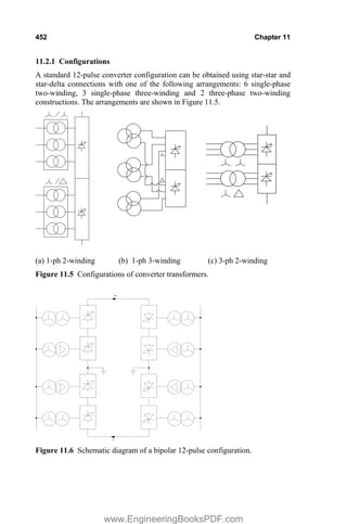
![Special Transformers 453
The weight and size of an individual transformer are highest and the overall cost
(with all transformers considered) is lowest in the three-phase two-winding
configuration, whereas the weight and size of an individual transformer are
lowest and the overall cost is highest in the single-phase two-winding
configuration. Since the cost of a spare transformer in the single-phase two-
winding configuration is lowest (that of only one of the six transformers), it is
more commonly used.
11.2.2 Insulation design
A simplified schematic diagram for bipolar (double) 12-pulse operation is
shown in Figure 11.6. The windings connected to the converters and that
connected to the AC side are generally termed as the valve and AC windings,
respectively. Since the potentials of the valve winding connections are
determined by the combination of conducting valves at any particular instant,
the entire valve winding has to be fully insulated. Also, unlike the AC windings,
both terminals of the valve windings experience the full DC voltage of the
bridge to which they are connected. Hence, the end insulation gaps are higher
resulting in greater radial leakage field at the two ends of the windings. The
winding eddy loss due to the radial leakage field can be much higher than that in
the conventional transformer, if the conductor dimensions are not chosen
properly.
Thus, in addition to the normal AC voltage, the valve windings are
subjected to a direct voltage depending on their position with respect to ground.
Under an AC voltage, the potential distribution is in inverse proportion to
capacitances, or electric stresses are inversely proportional to permittivities of
different insulating materials in a multi-dielectric system. Since the permittivity
of oil is about half of solid insulation, the stress in oil is more under the AC
voltage condition in the conventional transformers. Since the dielectric strength
of the oil is much less as compared to that of the solid insulation, the insulation
design problem reduces mainly to designing of oil ducts as elaborated in Chapter
8. Contrary to AC conditions, under DC voltage conditions the voltage
distribution is in direct proportion to resistances, or electric stresses are directly
proportional to resistivities of involved insulating materials. At lower
temperatures the resistivity of solid insulating materials used in transformers is
much higher than that of the oil. The ratio of the resistivity of a high quality
pressboard to that of the oil is about 100 at 20°C, which reduces to as low as 3.3
at 90°C [13]. This is because the fall in the resistivity of the pressboard with
temperature is much higher than that of the oil [14]. Such a large variation in the
ratio of the two resitivities increases the complexity of insulation design.
Thus, under DC conditions at lower temperatures, most of the voltage is
distributed across the solid insulation, and stress in it greatly exceeds that in the
oil. The oil ducts have practically only AC voltage across them, whereas solid
insulations (barriers, washers, supporting and clamping components, etc.)
www.EngineeringBooksPDF.com](https://image.slidesharecdn.com/transformer-engineering-design-technology-and-diagnostics-second-edition-pdf-230506172819-680afe24/85/transformer-engineering-design-technology-and-diagnostics-second-edition-pdf-pdf-474-320.jpg)
![454 Chapter 11
generally have a preponderance of DC voltage with a certain amount of
superimposed AC voltage. Therefore, the number of pressboard barriers is
greater in converter transformers as compared to conventional transformers.
However, the proportion of solid insulation cannot be higher than a certain value
because the composite oil-solid system has to withstand AC voltage tests as
well.
Let the symbols H and U denote relative permittivity and resistivity,
respectively. With voltage V across two parallel plates shown in Figure 11.7,
under AC field conditions the stresses in the oil and the solid insulation are
oil
for
d
d
V
E
2
2
1
1
1
H
H
solid
for
d
d
V
E
1
1
2
2
2
H
H
(11.6)
and under DC field conditions the stresses are
oil
for
d
d
V
E
2
1
2
1
1
U
U
solid
for
d
d
V
E
1
2
1
2
2
U
U
. (11.7)
For nonuniform field conditions involving complex electrode shapes, the
techniques described in Chapter 8 should be used to calculate the stresses.
Under steady-state DC conditions, space charges are accumulated at the
boundary of the oil and the solid insulation. When there is polarity reversal, in
which the applied DC voltage changes from V
to V
, an equivalent of the
voltage difference V
2 is applied. As the time required for reversing the polarity
of the applied voltage is much shorter than the space charge relaxation time [15],
the voltage due to space charge is not affected during the time of polarity
reversal. Therefore, using Equations 11.6 and 11.7, the stresses in the oil and the
solid insulation under the polarity reversal condition can be given by
solid
insulation
oil
V
' '
d d
1 2
H U U
H
1 2 2
1
Figure 11.7 Oil-solid insulation system.
www.EngineeringBooksPDF.com](https://image.slidesharecdn.com/transformer-engineering-design-technology-and-diagnostics-second-edition-pdf-230506172819-680afe24/85/transformer-engineering-design-technology-and-diagnostics-second-edition-pdf-pdf-475-320.jpg)
![Special Transformers 455
1
2 1
1 2 1 2
1 2
2
V V
E for oil
d d d d
U H
U H
c
(11.8)
2
1 2
2 1 2 1
2 1
2
V V
E for solid
d d d d
U H
U H
c
. (11.9)
Thus, under the polarity reversal condition, the oil gap is stressed more (since
1
2 U
U !! and 5
.
0
2
1 #
H
H ). It can be easily seen from the above equations that
the smaller the stress across the oil gap before the polarity reversal, the more the
stress is across it after the polarity reversal. The voltage distribution under
various conditions is shown in Figure 11.8. The voltage across the oil gap is
much higher during the polarity reversal condition (Case 3) as compared to Case
2 of the steady-state DC voltage condition (prior to the polarity reversal).
For the oil-solid composite insulation system, superimposition of a
relatively low DC voltage on an AC voltage has very little effect on the partial
discharge inception voltage [14-17]; this is due to the fact that most of the DC
voltage is dropped across the solid insulation, which has a high DC withstand
voltage. If, however, the DC voltage magnitude is within the range of the
breakdown voltage, the breakdown behavior of the entire system is determined
by the DC voltage. Although the converter transformers are stressed by
combined AC and DC voltages during service conditions, it is not considered
necessary to test them with superimposed voltages [18]. Conventional power
frequency and impulse tests are generally sufficient in addition to pure DC
voltage tests and the polarity reversal test.
-V
oil solid
potential
+V
2
1
3
Figure 11.8 Voltage distribution under various conditions [15].
1: capacitive
2: resistive
3: polarity reversal
www.EngineeringBooksPDF.com](https://image.slidesharecdn.com/transformer-engineering-design-technology-and-diagnostics-second-edition-pdf-230506172819-680afe24/85/transformer-engineering-design-technology-and-diagnostics-second-edition-pdf-pdf-476-320.jpg)
![456 Chapter 11
As in the case of AC insulation design (Chapter 8), the stresses under DC
voltage conditions can be calculated accurately by numerical methods. The field
distribution is generally calculated for a worst case condition, say at 20°C, since
at this temperature the ratio of the resistivity of the solid insulation to that of the
oil is high resulting in a high stress value in the solid insulation. The density of
equipotential lines in barriers/cylinders is much higher compared to that in the
oil, necessitating an increase in their thickness compared to that in conventional
transformers. The shape and placement of barriers and the width of the resulting
oil ducts would have already been decided by the requirements of AC design
and thermal considerations [13]. Hence, it is obvious that the high strength of
the solid insulation cannot be fully utilized from the DC design consideration if
the stress in the oil gap (having a lower strength) has to be kept low under the
AC and polarity reversal conditions [19]. Discontinuities in solid insulations
result in higher tangential (creep) stresses along the solid-oil interfaces, and
hence these should be properly looked at while finalizing the insulation design.
The insulation design of the converter transformers is complicated by the
fact that the ratio of resistivities of the solid insulation and the oil, which varies
considerably as explained earlier, is greatly influenced by a number of factors
[18], such as temperature, field strength, moisture, time, and aging (contrary to
the conventional transformers where the corresponding ratio of permittivities
does not exceed about 2 and is practically independent of external factors).
The volt-time characteristics of the oil under DC voltage conditions are
reported in [15, 20] for plane-plane electrodes; the DC breakdown voltage
shows a rapid rate of decrease for stressing time until 100 seconds, after which
there is hardly any decrease. The long-time breakdown voltage (t f
o ) is 70 to
80% of the one-minute breakdown voltage [20]. Under combined AC-DC
voltage conditions, the AC breakdown voltage of the oil decreases as the DC
voltage increases. The DC 1-minute withstand voltage of the oil gap is about 20
to 30% lower than the AC 1-minute withstand voltage [16, 20, 21]; on the
contrary the oil-impregnated paper/solid insulation withstands more DC voltage
than AC voltage [16]. A higher DC strength of the solid insulation can be partly
explained by the absence of partial discharges which lower the strength in the
case of AC voltages. Even if there are oil voids in the solid insulation, the stress
in them is too low under the DC voltage to initiate partial discharges.
It is reported in [22] that the dielectric strength of the converter
transformer insulation under the polarity reversal condition is similar to that
under switching impulse stresses. An equivalent AC power frequency voltage
test has been suggested for the polarity reversal test.
From the typical schematic shown in Figure 11.6, it is clear that when a
number of converters are connected in series, the line (AC side) windings are
connected in parallel across the same lines and the inductively transferred
overvoltage to ground increases cumulatively from one converter bridge to the
next higher bridge because the valve (DC side) windings are connected in series
www.EngineeringBooksPDF.com](https://image.slidesharecdn.com/transformer-engineering-design-technology-and-diagnostics-second-edition-pdf-230506172819-680afe24/85/transformer-engineering-design-technology-and-diagnostics-second-edition-pdf-pdf-477-320.jpg)

![458 Chapter 11
Under normal operating conditions, the current in the converter
transformer windings has a stepped waveform. It is still an AC current since it is
symmetrical about the x axis. Nonuniformities or asymmetries in valve firing
angles produce DC magnetization of the transformer core increasing the
magnetizing current, and the windings carry a DC current component
corresponding to the level of DC magnetization. Although with modern firing
controls, the DC magnetization is much lower, careful design of the magnetic
circuit is necessary to avoid excessive losses and noise in the core.
Due to harmonics and possibilities of DC magnetization, the operating
flux density in the converter transformer is less than that in the conventional
transformer, and its value is around 1.6 Tesla. A high harmonic content
produces greater noise, and some special measures for noise control may have to
be adopted as described in Chapter 10.
The leakage field in converter transformers contains appreciable harmonic
content which results into high eddy losses in windings and structural parts. The
losses in the windings can be controlled by using subdivided conductors or CTC
(continuously transposed cable) conductors. If the CTC conductors are used,
they are an epoxy-bonded type having high short-circuit strength as explained in
Chapter 6. The magnetic or eddy current shielding techniques, discussed in
Chapter 5, have to be used to minimize losses and to eliminate hot spots in the
tank and other structural components. The load loss of a 213 MVA single-phase
converter transformer has been measured at a number of frequencies between 60
Hz and 6 kHz in the work reported in [23]; the corresponding harmonic load loss
factors are given for accounting extra losses due to harmonics.
Short-circuit withstand: Due to possibility of maloperations of valves resulting
in high currents, the short-circuit withstand design of the converter transformers
deserves more attention. Quality of processing (drying and impregnation) and
integrity of clamping/support structures have to be ensured. The windings of the
converter transformers need to be adequately braced. The current density of the
windings can be lower to enhance their strength against short-circuit forces.
11.3 Furnace Transformers
A transformer supplying an arc furnace has to deliver unusually high currents
over a wide range of voltage. Power ratings between 50 and 100 MVA are quite
common now with the secondary currents of more than 50 kA. Furnace
transformers have special features for handling very high currents compared to
conventional transformers. Since the LV winding current is high, its voltage is
better controlled by providing taps on the HV winding.
An arc furnace has three electrodes connected to the secondary terminals
of the furnace transformer which has to be specially designed to withstand
frequent short circuits on the secondary side. Currents drawn in the arc furnace
are characterized by wide fluctuations and unbalanced conditions, which lead to
www.EngineeringBooksPDF.com](https://image.slidesharecdn.com/transformer-engineering-design-technology-and-diagnostics-second-edition-pdf-230506172819-680afe24/85/transformer-engineering-design-technology-and-diagnostics-second-edition-pdf-pdf-479-320.jpg)
![Special Transformers 459
problems of voltage drops, harmonics, etc. (details are given in Section 13.4)
These effects can be mitigated by supplying furnaces directly from a high
voltage transmission line having high capacity (i.e., an adequate short-circuit
level at the supply point) through a furnace transformer. In such a case, when the
voltage ratio is high, suitable measures should be taken for protecting the
secondary winding against the electrostatically transferred voltages from the
high voltage primary winding. These measures are connection of a surge
arrester, or a capacitor, between the secondary terminals and a ground and
placement of an electrostatic shield between the primary and secondary
windings.
The leakage reactance of the furnace transformer affects the furnace
operation since it is added to the reactance of the high current connections
between the transformer secondary terminals and electrode tips. The higher the
reactance, the lower the useful service currents are, thereby reducing the
efficiency of the operation. Hence, the leakage reactance needs to be kept as
small as practically possible with due consideration to the short-circuit withstand
of windings and clamping/support structures. Also, a certain minimum value of
reactance is required in the furnace circuit to stabilize arcs. In large furnace
installations, the low voltage connections usually provide the necessary
reactance. For smaller installations, a reactor may have to be added in series
with the primary winding to give a sufficient reactance value for the stability.
The series reactor, which may be housed in the tank of the furnace transformer,
is usually provided with taps so that the reactance value can be varied for an
optimum performance. Hence, depending on the rating of furnace installation
and its inherent reactance, the leakage reactance of the furnace transformer has
to be judiciously selected to meet the stability and efficiency requirements.
Although the core-type construction is common, the shell-type
construction is also used [24] because one can get a desired low impedance
value by suitably interleaving the primary and secondary windings. The furnace
transformers are provided with a separate regulating (tap) winding. The
variation of the percentage reactance over the entire tapping range depends on
the disposition of the windings. The effects of various dispositions on the
percentage reactance and the performance of furnaces are analyzed in [25].
The melting process of a furnace requires initially more power to break
down and melt the furnace charge. The power required afterward for refining the
molten metal is lower. The variable power input requirement is achieved by
varying the supply voltage to the electric arc furnace over a wide range
continuously using an OLTC. Its use is essential where temporary interruptions
in supply for changing taps is not desirable. Since the regulation required is
generally fine, an OLTC with a large number of steps is required. Due to
frequent operations, its oil quality should be regularly checked. It is preferable to
place the OLTC in a separate compartment so that its maintenance can be
carried out without having to lower the oil to an extent that windings are
exposed [26].
www.EngineeringBooksPDF.com](https://image.slidesharecdn.com/transformer-engineering-design-technology-and-diagnostics-second-edition-pdf-230506172819-680afe24/85/transformer-engineering-design-technology-and-diagnostics-second-edition-pdf-pdf-480-320.jpg)


![462 Chapter 11
main
transformer
booster
transformer
Figure 11.10 Figure eight connection.
Also, the two windings are often connected in a figure eight fashion (Figure
11.10) avoiding extra connections between them. A special arrangement is
required to lift the two core-winding assemblies simultaneously.
Since the current carried by the secondary windings is quite high, a
continuously transposed cable (CTC) conductor is used which minimizes the
eddy losses, gets rid of the transposition problems, and improves the winding
space factor. The material of structural parts supporting high current
terminations and tank parts in the vicinity of high current fields should be non-
magnetic steel. Analysis of a high current termination in a large furnace
transformer is reported in [27], wherein excessive losses and hot spots observed
during the tests have been analyzed by 3-D FEM analysis. Suitable
modifications in magnetic clearances and the tank material eliminated the hot
spots.
The secondary winding of a furnace transformer is made up of a number
of parallel coils arranged vertically and connected by vertical copper bars. A go-
and-return arrangement is used for the input and output connections (placed
close to each other) reducing the magnetic field and associated stray losses in
the nearby structural parts. A delta-connected secondary winding is preferable
since the current to be carried by it is reduced. Many times, both the ends of
each phase of the secondary winding are brought out through the terminals and
the delta connections are made at the furnace (i.e., the connections are
automatically formed by the metallic charge in the furnace). This minimizes the
inductive voltage drops in the leads and can achieve a better phase balance
www.EngineeringBooksPDF.com](https://image.slidesharecdn.com/transformer-engineering-design-technology-and-diagnostics-second-edition-pdf-230506172819-680afe24/85/transformer-engineering-design-technology-and-diagnostics-second-edition-pdf-pdf-483-320.jpg)
![Special Transformers 463
between the electrode currents. Due to heavy connections, some unbalance may
exist which has to be minimized by some specific arrangements [25]. The
secondary winding terminals are usually located on the vertical side of the tank
(instead of the top cover) resulting in lower lengths of the connections, stray
losses, and the transformer cost. The LV (secondary) winding is invariably the
outermost winding and the HV (primary) winding can be placed next to the core.
In such a case, the regulating (tap) winding is between the HV and LV windings.
Such a disposition of windings reduces variations in the percentage impedance
as the tap position is changed from the minimum to the maximum in variable
flux designs.
Small furnace transformers are naturally cooled with radiators. For large
ratings and where there are space restrictions, forced oil cooling with an oil-to-
water heat exchanger can be used. The oil pressure is always maintained higher
than the water pressure (so that the water does not leak into the oil if a leakage
problem develops). The LV terminations may be in the form of U-shaped copper
tubes of certain inside and outside diameters so that they can be water cooled
from inside. These copper tubes can be cooled by oil as well [26].
11.4 Phase Shifting Transformers
In a complex power transmission network, a phase shifting transformer (PST)
can be used to control the flow of active power and to improve transient stability
in a very efficient way as elaborated in Section 13.1.2. It has been successfully
used to control and increase the power flow between two large systems [28]; in
this case the option of using a PST was finalized after its comparison with other
options such as an HVDC link and series capacitors. The PST provides a well-
defined phase shift (advance or retard) between the primary (source) and
secondary (load) terminals as shown in Figure 11.11. In the phase-advance
mode, the voltage vector at the output of the PST is made to lead the input
voltage vector by adding a leading quadrature voltage to the source voltage. In
the phase-retard mode, a lagging quadrature voltage is added to the source
voltage so that the voltage vector at the output of the PST lags the input voltage.
VL VS VS
VL
V
' V
'
D D
S
PST
L
phase rotation
Advance Retard
Figure 11.11 Advance mode and retard mode.
www.EngineeringBooksPDF.com](https://image.slidesharecdn.com/transformer-engineering-design-technology-and-diagnostics-second-edition-pdf-230506172819-680afe24/85/transformer-engineering-design-technology-and-diagnostics-second-edition-pdf-pdf-484-320.jpg)
![464 Chapter 11
Normally, the phase shift can be varied during operation in definite steps
by use of an OLTC. The sign of the phase shift can be inverted by using an
OLTC having a reversing switch. These transformers can be constructed with
many different winding configurations depending on the rated voltage, the
power output, and the amount of required phase shift.
The rated power that decides the PST size is given by [29]
^ ` 2
sin
2
3
2
sin
2
3 D
D u
u
u
u SL
ph
SL
ph
eq I
V
I
V
S (11.10)
where ph
V is the line-to-ground voltage, SL
I is the line current flowing from the
source to the load, and the term in the brackets is the voltage between S and L
terminals expressed in terms of the phase shift angle D . Hence, the required
maximum value of the phase shift angle decides the rating and size of the PST.
Depending on the voltage/power rating, phase shift angle requirements,
connected system’s short-circuit capability and OLTC performance, two distinct
designs of PST are used, viz. single-core design and double-core design.
The simpler single-core design is generally used at lower voltages for
small phase shifts and small ratings of PSTs. Figure 11.12 shows the
arrangement of a PST with a delta-connected exciting winding. In this
configuration, the regulating winding of each phase is wound on the same core
limb as the exciting winding. The phase shift between the source (S) and load
(L) terminals is achieved by connecting the regulating winding as shown in the
figure. Its voltage is in phase with that of the exciting winding between the other
two phase terminals. The voltage magnitudes of the S and L terminals are equal
under the no-load condition. The phasor diagram shows the phase shift
advancement obtained for the load terminal voltage with respect to the source
terminal voltage. If an OLTC with a reversing switch is used, one can obtain a
phase-advance position as well as a phase-retard position.
Ve
VSR
VLR
VRR2
R1 R2
S L
L
L
S
S
D
VR1R
R
R
Y
B B
R
Y
Figure 11.12 Delta configuration of PST and phasor diagram.
www.EngineeringBooksPDF.com](https://image.slidesharecdn.com/transformer-engineering-design-technology-and-diagnostics-second-edition-pdf-230506172819-680afe24/85/transformer-engineering-design-technology-and-diagnostics-second-edition-pdf-pdf-485-320.jpg)
![Special Transformers 465
V
e
VAA’
VSR VLR
A
A’
D
S L S L S L
R R Y Y B B
Figure 11.13 Delta-hexagonal PST (with retard phase shift).
A special case of the configuration shown in Figure 11.12 is the design
with only one tap winding and one OLTC with a reversing switch, which can be
used for smaller phase shifts.
Another configuration that uses the single-core design is shown in Figure
11.13. The arrangement, known as delta-hexagonal PST, generally has an OLTC
with linear regulation, i.e., without a reversing switch. The regulating winding is
wound on the same core limb as the main exciting winding. The regulating
winding of the R phase is located between the main windings of the Y and B
phases and produces a phase shift (retard) as shown in the figure.
The two configurations of the single-core design discussed above have
line-end regulation. The tap changer and the regulating (tap) winding are
directly exposed to system disturbances (overvoltages/short-circuit currents).
Hence, the cost of the OLTC increases. Additional impedances may have to be
connected to the load side terminals to protect the tap changer from short-circuit
currents because no transformer impedance is present at zero phase angle. If an
OLTC with a reversing switch is used in the arrangement shown in Figure
11.12, during the switch operation, the tap winding is momentarily disconnected
from the main winding. Its potential is then decided by the potentials of adjacent
windings and the capacitances between the windings and between the windings
and ground. This problem of high recovery voltage can be tackled [29, 30] by
using shields between the windings or by using a tie-in resistor (which connects
the tap winding to a fixed potential during the reversing operation).
www.EngineeringBooksPDF.com](https://image.slidesharecdn.com/transformer-engineering-design-technology-and-diagnostics-second-edition-pdf-230506172819-680afe24/85/transformer-engineering-design-technology-and-diagnostics-second-edition-pdf-pdf-486-320.jpg)

![Special Transformers 467
It is clear from the phasor diagram that the voltage BB
V c also changes
with the phase angle D because the exciting winding ( BBc ) is located
electrically in the middle of the series winding. For q
0
D , AA
V c becomes zero
and the three voltages SR
V , LR
V and BB
V c become equal. Thus, the condition
q
0
D gives the highest exciting voltage BB
V c , and the corresponding voltage
at the tap winding is also maximum. The OLTC has to be designed for the step
voltage corresponding to this highest voltage.
In order to achieve rapid and smooth control of the power flow, static
phase shifters can be used, which employ tap changers consisting of static
devices like thyristors. One such scheme, reported in [31], is shown to minimize
the subsynchronous resonances in large turbine-generators occurring due to
capacitive series compensation of lines. Applications of static phase shifters in
power systems are reported in [32]. By augmenting an existing conventional
phase shifter with a small static phase shifter (thus giving a hybrid phase
shifter), dynamic performance can be improved.
The calculation of currents in phase shifting transformers under system
fault conditions requires more elaborate treatment as compared to that for
conventional transformers. The equivalent circuit model and the positive-
sequence, negative-sequence and zero-sequence networks under the fault
analysis are explained in [33]. The reported method can be used to calculate
currents under various fault conditions.
References
1. Schaefer, J. Rectifier circuits: theory and design, John Wiley and Sons,
Inc., New York, 1965.
2. Pelikan, T. and Isler, J. Rectifier transformers for heavy currents, The
Brown Boveri Review, Vol. 48, No.3/4, March/April 1961, pp. 215–228.
3. Wells, R. Rectifier interphase transformers and current balance, Electrical
Review, Vol. 207, No. 14, October 1980, pp. 45–46.
4. Bhide, R. S., Kulkarni, S. V., and Bhandarkar, P. Analytical description for
zero-sequence characteristics of five-legged core construction in
Transformers, Proceedings of IET — Electric Power Applications, Vol. 4,
No. 6, July 2010, pp. 407–417.
5. Bhide, R. S., Kulkarni, S. V., and Bhandarkar, P. Analysis of five-legged
transformer used for parallel operation of rectifiers by coupled circuit-field
approach, IEEE Transactions on Power Delivery, Vol. 26, No. 2, April
2011, pp. 607–616.
6. Coppadoro, F. Voltage regulation of transformers for silicon rectifiers,
Brown Boveri Review, Vol. 8-72, August 1972, pp. 416–421.
www.EngineeringBooksPDF.com](https://image.slidesharecdn.com/transformer-engineering-design-technology-and-diagnostics-second-edition-pdf-230506172819-680afe24/85/transformer-engineering-design-technology-and-diagnostics-second-edition-pdf-pdf-488-320.jpg)


![472 Chapter 12
order to obtain accurate values of field variables and related performance figures,
source and boundary conditions have to be defined correctly. The mesh size has to
be small enough in the areas where the spatial rate of change of a field variable is
high. Many times 2-D approximations have to be done since 3-D field
computations are computationally demanding. Nonlinear transient 3-D problems
may have convergence problems. The knowledge of the product, fields and
numerical techniques is essential for doing reasonable 2-D approximations.
Commercial software programs offer alternative formulations for 3-D simulations;
competence in computational electromagnetics is certainly necessary to apply
them. Numerical results need to be verified by approximate analytical or empirical
formulae at least initially while using commercial software.
The above discussion underlines the need of giving an adequate exposure of
the field theory and FEM to transformer engineers. This is exactly the motivation
of this chapter; basics of electromagnetics as relevant to transformer engineering
are discussed first. The idea is not to describe the field theory in detail; it is
exhaustively covered in numerous textbooks on the subject [1–4]. Rather,
emphasis is given on summarizing the pertinent theory that would be useful to the
engineers while analyzing various electromagnetic phenomena in transformers.
After giving a brief introduction to Maxwell’s equations, the second section
describes the mathematical concepts which are the main foundations of the field
theory. Later, potentials used for solving electrostatic, magnetostatic, and time
varying problems are elaborated. The most popular numerical technique, FEM, is
then explained with examples. Various field formulations and their applications
for performance assessment of transformers, under steady state and transient
conditions, are then summarized. Coupled field problems in transformers,
involving interaction between electromagnetic fields and circuits and/or physical
fields, are also described. The coupled problems in transformers involving circuit-
field, magnetic-thermal, and magnetic-structural phenomena are then elucidated.
Lastly, the performance figures that can be computed using the technique are
elaborated. This exposure to the field and FEM theory in this chapter is expected
to help researchers and practicing engineers to solve complex as well as practical
electromagnetic and coupled problems in transformers.
12.1 A Perspective
As discussed earlier, the transformer is a complex 3-D structure in which many
physical fields like thermal, fluid, structural, acoustic, etc., exist in addition to
electric and magnetic fields. If these fields can be represented accurately by an
equivalent lumped parameter representation, their spatial distribution is not
required to be known. However, it is a well-known fact that practical products
such as transformers cannot be reliably designed and/or optimized without the
precise knowledge of fields inside them. Empirical formulae fail to represent
distributions of the fields in space, particularly so in the problem regions with high
gradients. End effects, sharp corners, material nonlinearities and hysteretic
www.EngineeringBooksPDF.com](https://image.slidesharecdn.com/transformer-engineering-design-technology-and-diagnostics-second-edition-pdf-230506172819-680afe24/85/transformer-engineering-design-technology-and-diagnostics-second-edition-pdf-pdf-493-320.jpg)


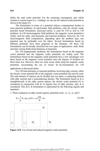


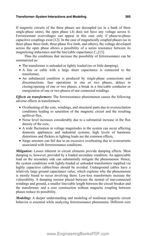


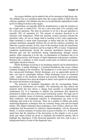


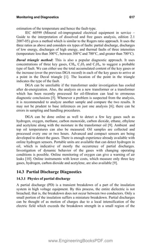


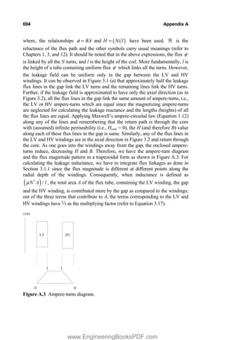


![Chapter_3-Transformers[1]-1.pdf](https://cdn.slidesharecdn.com/ss_thumbnails/chapter3-transformers1-1-230622173423-be6efc48-thumbnail.jpg?width=640&height=640&fit=bounds)


![Alan Lucas - [Template] [Template] [Template] ScienceFairProjectTemplate.pptx](https://cdn.slidesharecdn.com/ss_thumbnails/alanlucas-templatetemplatetemplatesciencefairprojecttemplate-260106222421-b6ad9ab7-thumbnail.jpg?width=640&height=640&fit=bounds)


