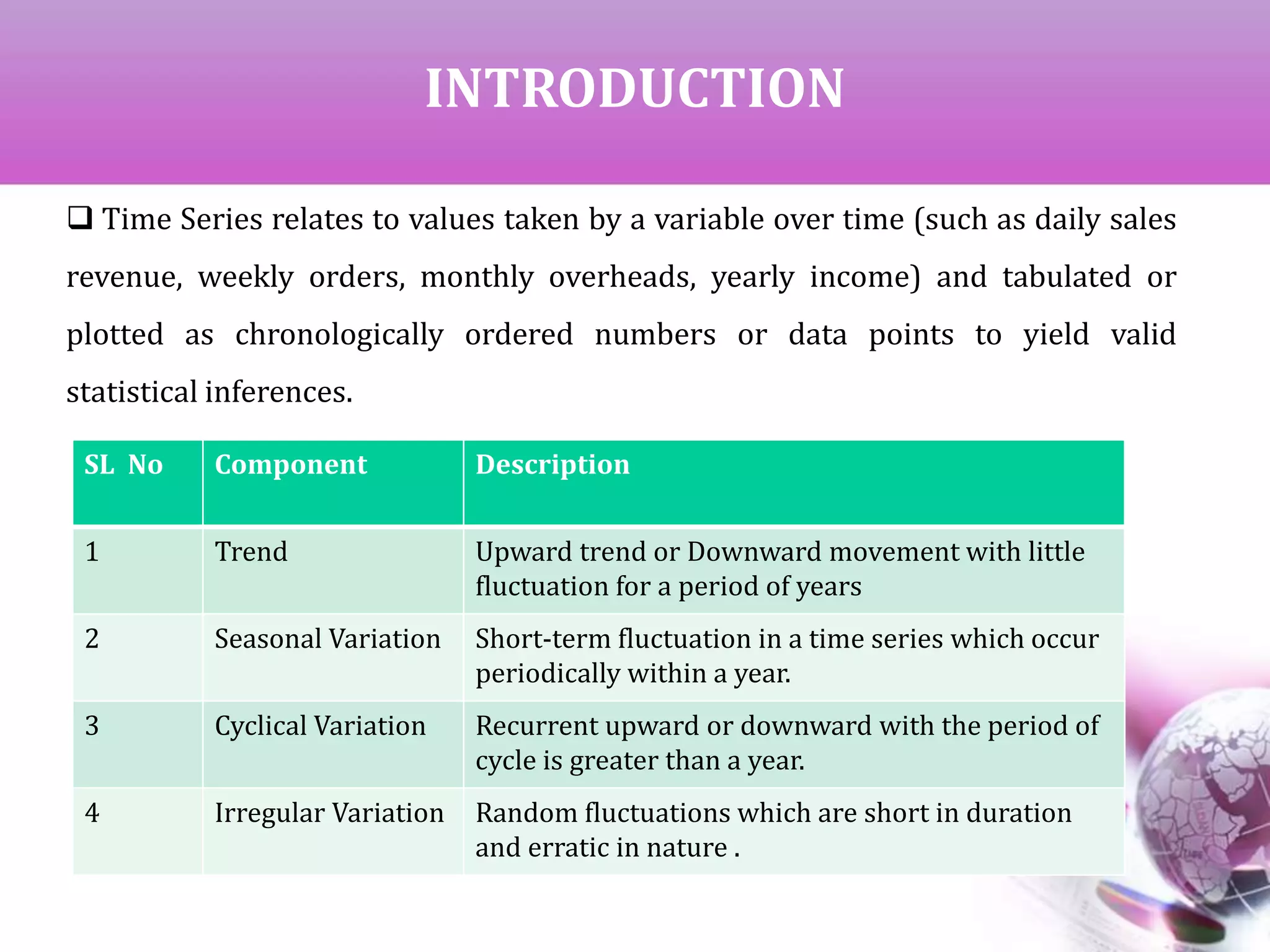
![DATA PREPARATION
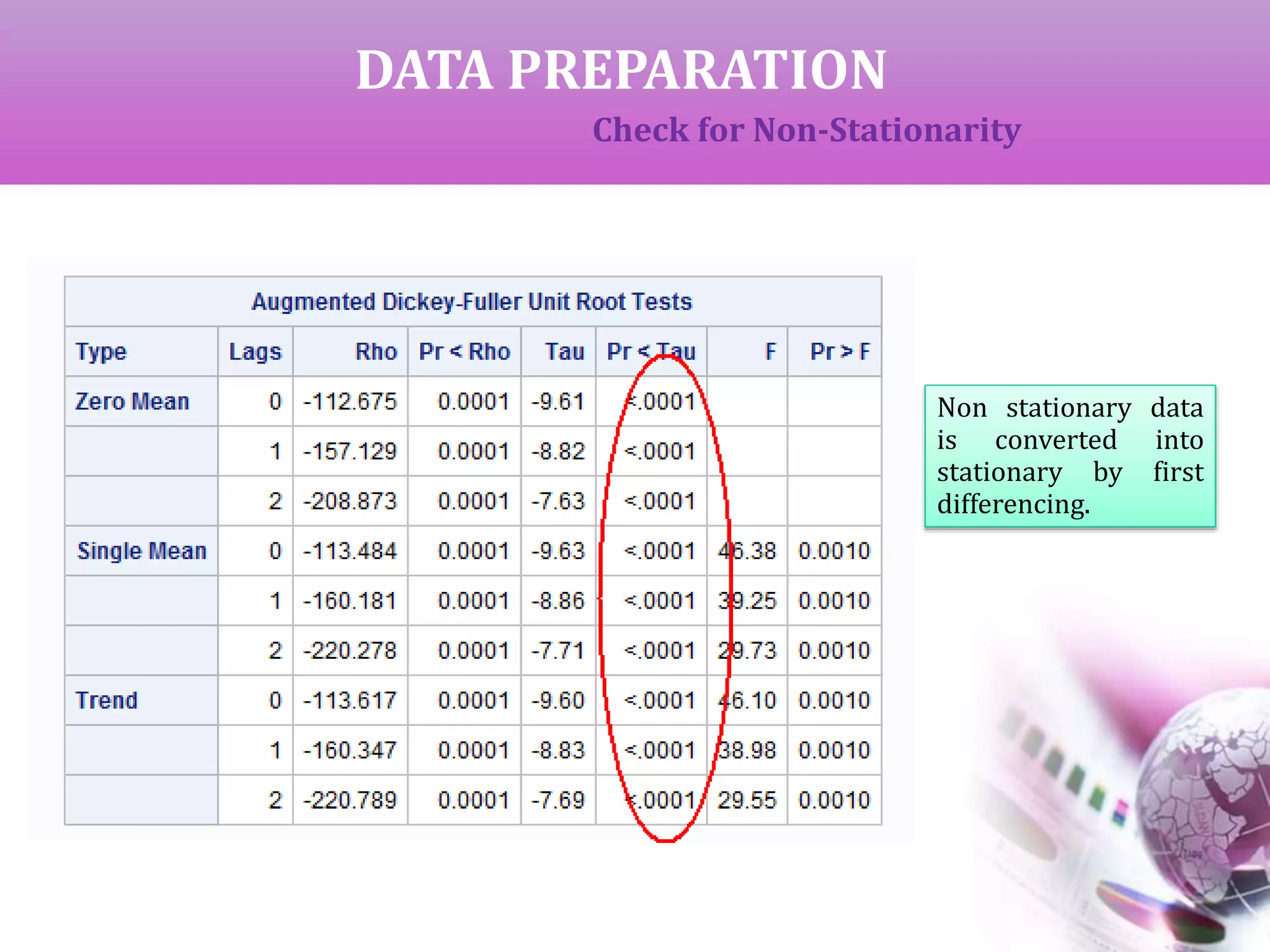
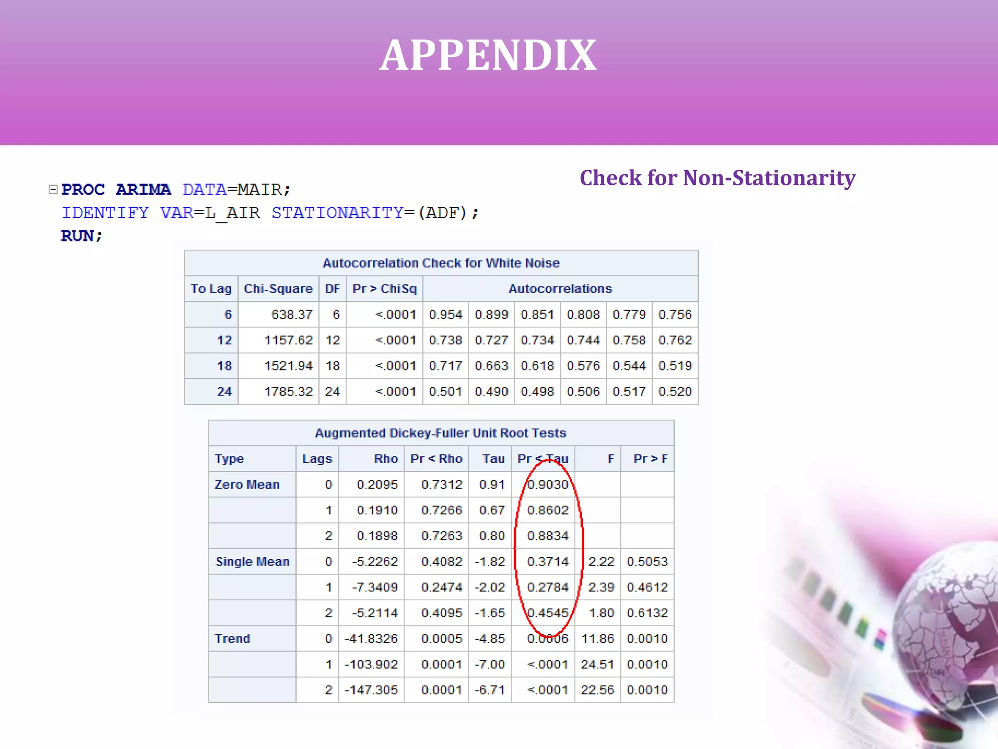
Check for Non-Stationarity
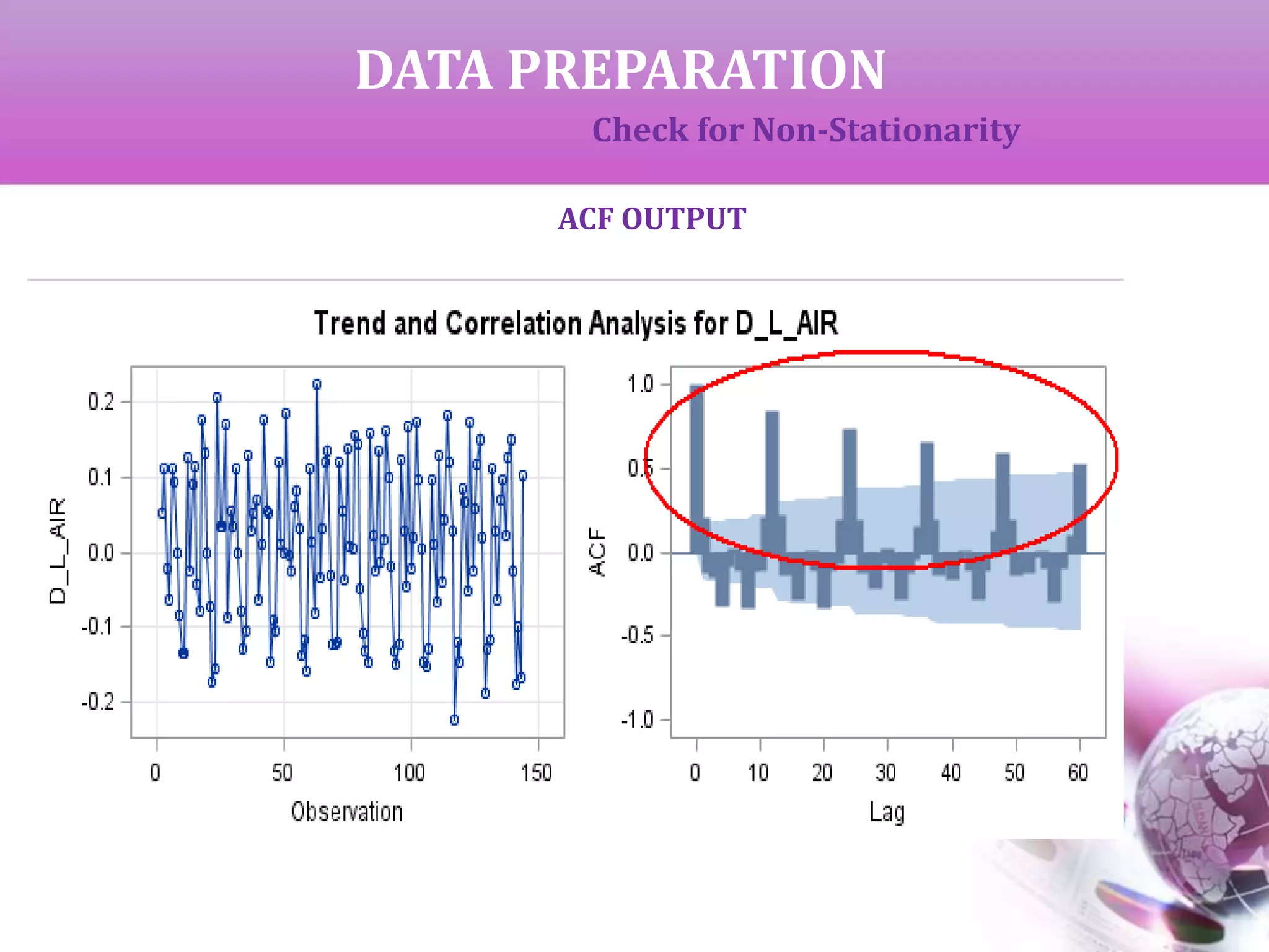
If the data is completely random with no fixed pattern, it is called non-
stationary data and cannot be used for future forecasting. This is checked
by ‘Augmented Dickey-Fuller Unit Root Test’ (ADF).Here,
H0 : Data is non-stationary
If p < alpha, we reject H0 to claim that the data is stationary and
hence
can be used for forecasting.
If p > alpha, we get non-stationary data which can be converted to
stationary by successive differencing.
We can start with first difference (y[t]-y[t-1]) which can obtained using
DIF(L_AIR) or L_AIR(1).Similarly, if we need second difference, it is
DIF2(L_AIR) .](https://image.slidesharecdn.com/timeseriesanalysis-140408021726-phpapp02/75/Time-Series-Analysis-Modeling-and-Forecasting-8-2048.jpg)
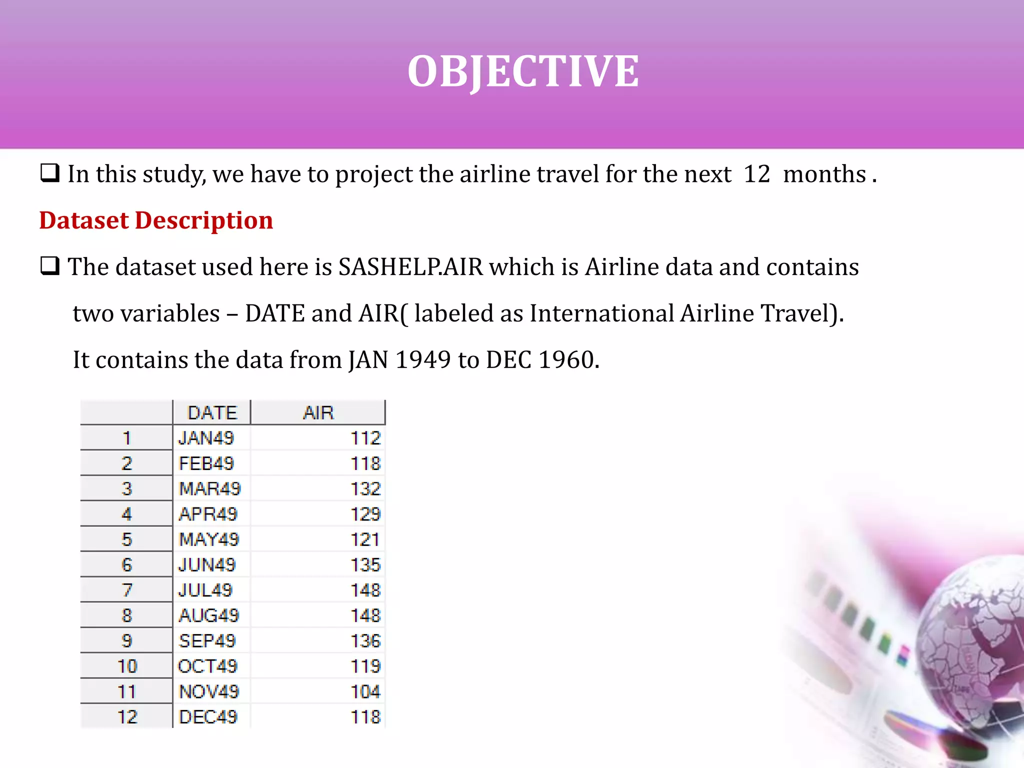
![DATA PREPARATION
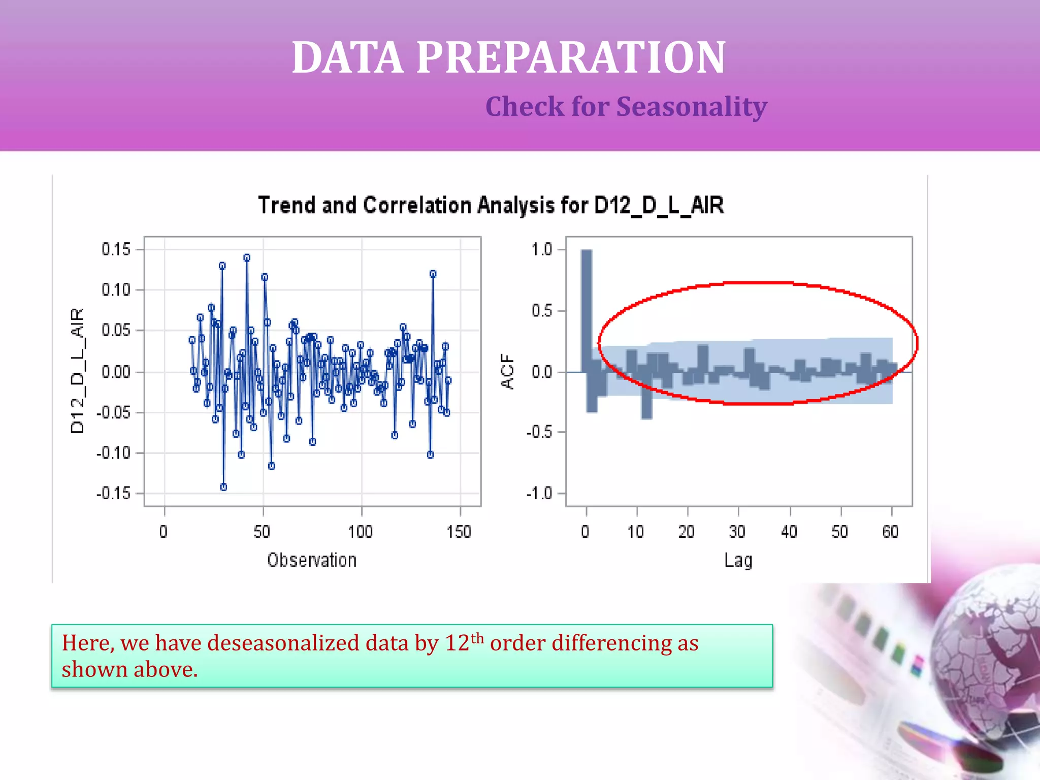
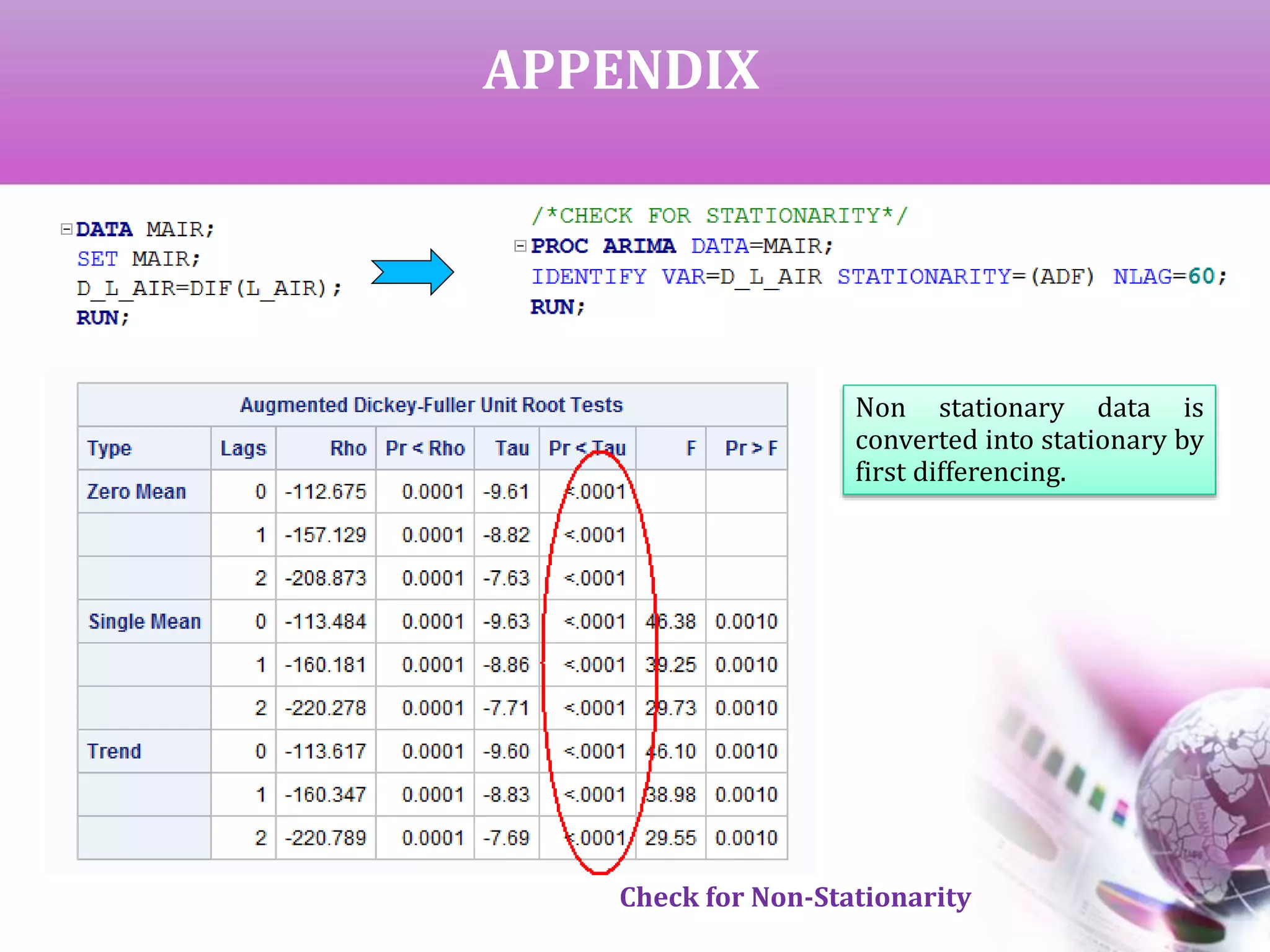
Check for Seasonality
The Auto Correlation function (ACF) gives the correlation between
y[t]-y[t-s] where ‘s’ is the period of lag.
If the ACF gives high values at fixed interval, that interval can be
considered as the period of seasonality. A differencing of same order
will deseasonalize the data.
From the output of ACF it can be observed that the period of
seasonality is 12 years.](https://image.slidesharecdn.com/timeseriesanalysis-140408021726-phpapp02/75/Time-Series-Analysis-Modeling-and-Forecasting-11-2048.jpg)
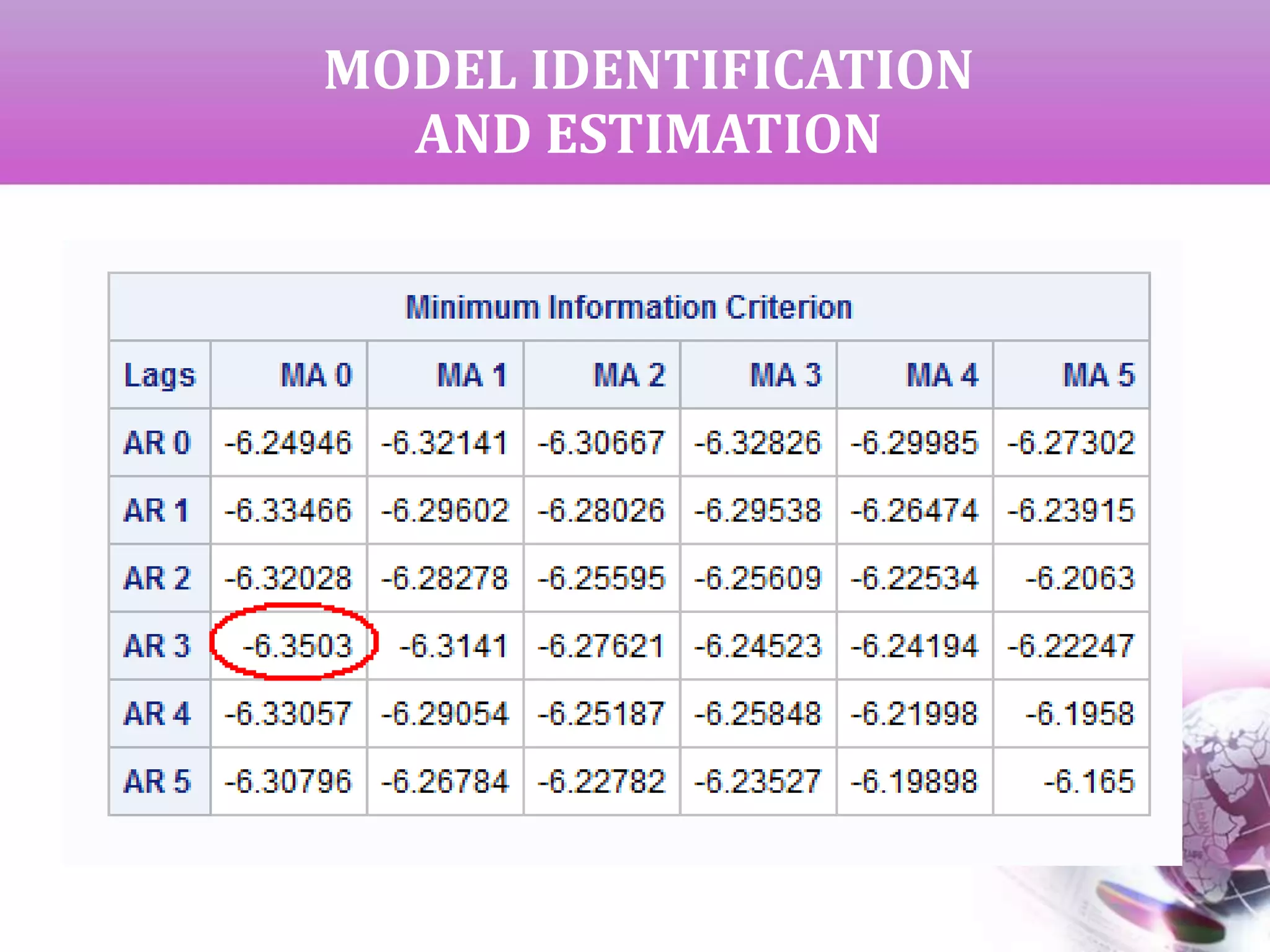

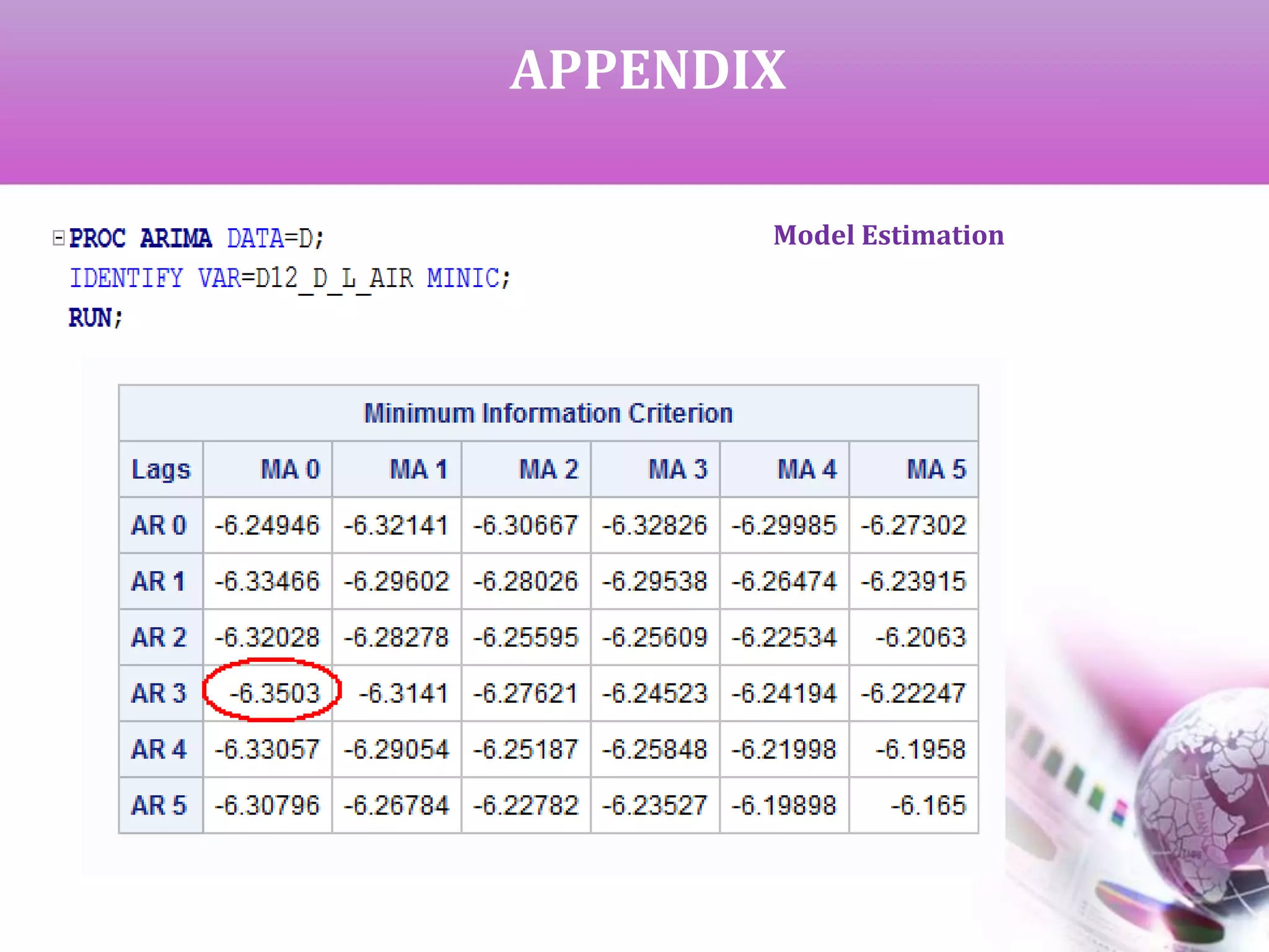
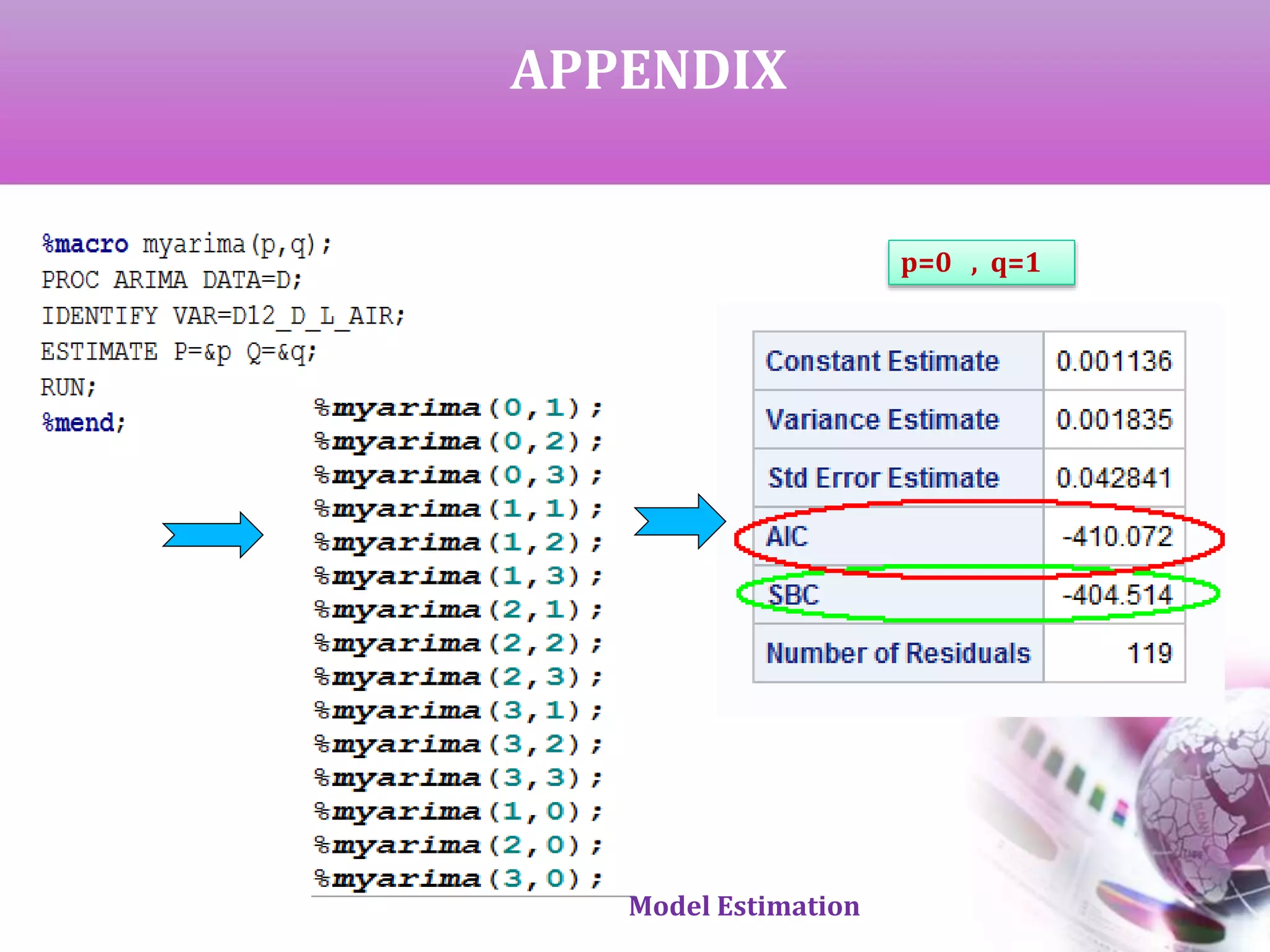
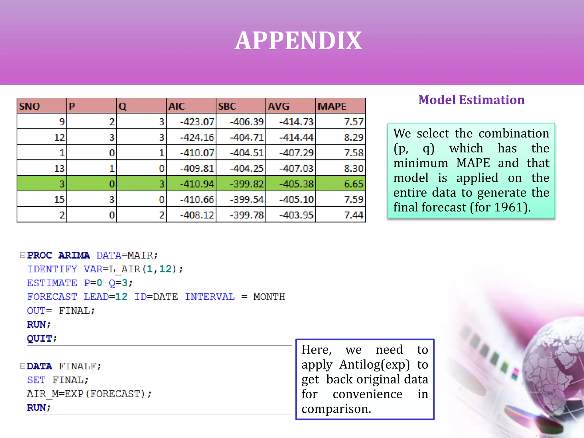
![MODEL IDENTIFICATION
AND ESTIMATION
AIC & SBC for all the neighborhood
models [ (0,1) to (3,3)]
Top 7 models based on lower
average value
Model Estimation](https://image.slidesharecdn.com/timeseriesanalysis-140408021726-phpapp02/75/Time-Series-Analysis-Modeling-and-Forecasting-16-2048.jpg)
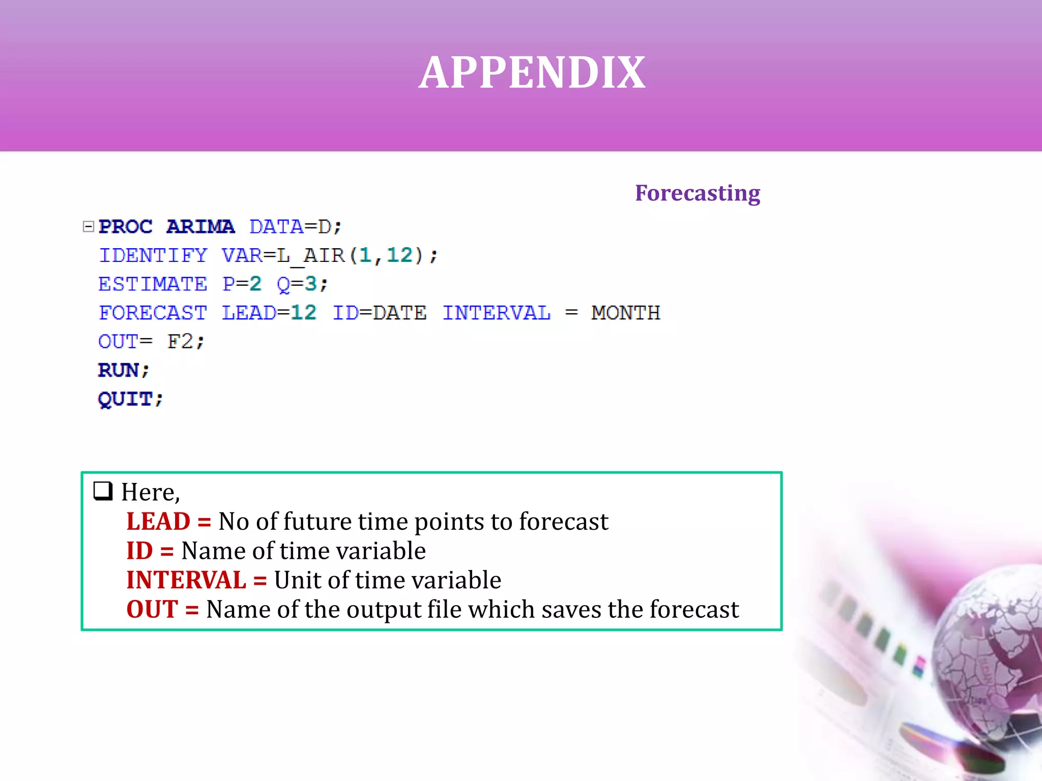
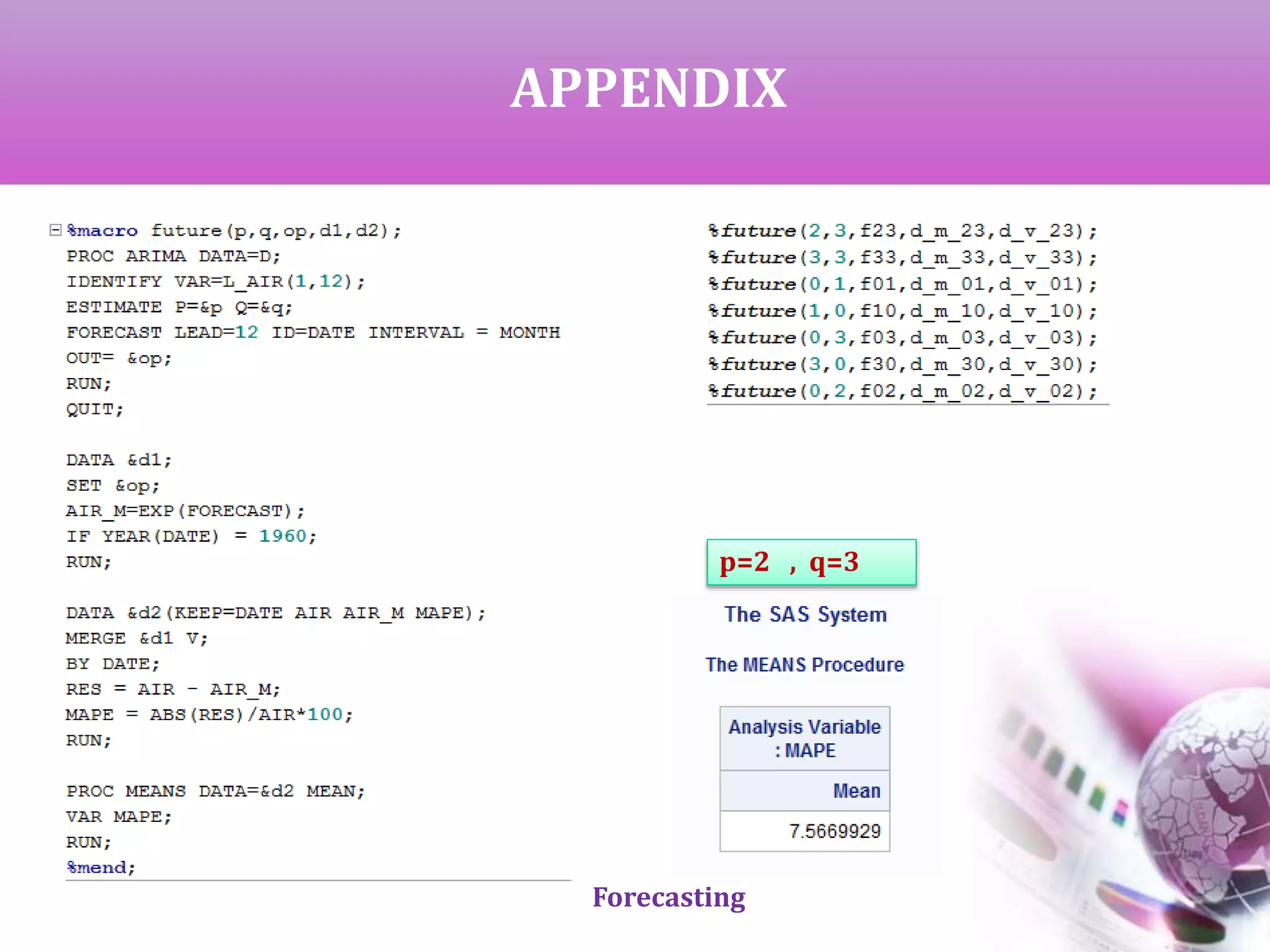


The document presents a study on time series analysis and forecasting of airline travel using the SAS dataset from January 1949 to December 1960. It details the methods for checking data volatility, non-stationarity, and seasonality, and describes the steps for model identification and estimation using the ARIMA framework. The final goal is to generate accurate forecasts for future airline travel based on the historical data analyzed.


![[DSC Europe 25] Marija Vlajkovic & Andrea Radonjanin - Integration of AI tool...](https://cdn.slidesharecdn.com/ss_thumbnails/qf1jrglttoc3bm8s3aop-final-integration-of-ai-tools-251208151905-394f3a6a-thumbnail.jpg?width=640&height=640&fit=bounds)


![[DSC Europe 25] Jim Sterne - Adopting Generative AI Capabilities Into the Ent...](https://cdn.slidesharecdn.com/ss_thumbnails/sxhpofuorcagxsaulkmt-3-251204082258-7e66bc48-thumbnail.jpg?width=640&height=640&fit=bounds)


![[DSC Europe 25] Vid Stimac - Policy Parsimony: Between Oversimplifying and Ov...](https://cdn.slidesharecdn.com/ss_thumbnails/eqlepagzqp2rhg3gbluh-dsc-stimac-251120-251205090438-059e7f54-thumbnail.jpg?width=640&height=640&fit=bounds)

![[DSC Europe 25] Dusan Jovicic - AI Story: From on-prem to cloud and back agai...](https://cdn.slidesharecdn.com/ss_thumbnails/8kp49m6uq22ifnbwhfnk-2-251205085715-964d11a6-thumbnail.jpg?width=640&height=640&fit=bounds)


![[DSC Europe 25] Dragan Vucic - Building the Learning Organization - How AI Tr...](https://cdn.slidesharecdn.com/ss_thumbnails/8brigo2sbu6qur6gxrra-7-251205085715-6ae07d24-thumbnail.jpg?width=640&height=640&fit=bounds)

