Autoregressive model
in financial time series
Mines ParisTech
Xiangnan YUE
Introduction
• Data visualization: the historical HS300 index from
2017.9 to 2017.11
Introduction
• In a case where no correlation is presented, it’s
called the white noise. (w(t)..)
Introduction
• Moving-average and autoregression are two ways
to introduce correlation and smoothness
• use 1/20 for [w(t-9),..,w(t),..,w(t +10)]
• autoregression
• x(t) = x(t-1) - 0.9x(t-2) + w(t)
Introduction
• Before using autoregression, the auto-correlation
and cross-correlation have to be checked.
• Auto-correlation is the relation between x(t+k) and
x(t), which is of the same time series.
• ACF(k) = cov(X(t+k), X(t)) / cov(X(t), X(t))
• cross-correlation is the relation between two time
series {x(n)} and {y(n)}
Introduction
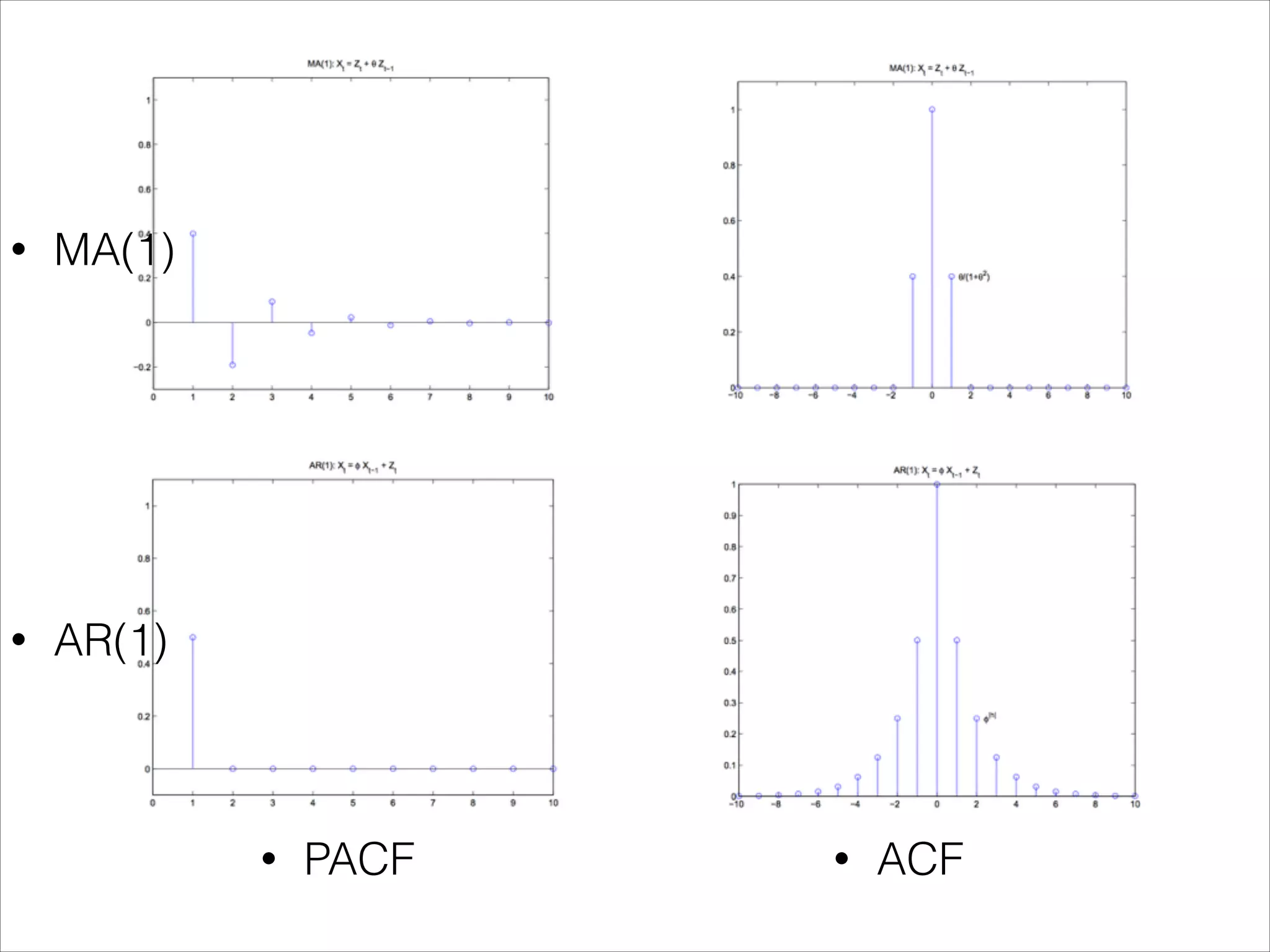
• sometimes we see also the PACF, which is used to
remove the influence of intermedia variables.
• for example phi(h) is defined as
• If we remember that E[X(h)|X(h-1)] can be seen as the
projection of X(h) to the X(h-1) plane, this PACF(h) can be
explained in the following graph
• MA(1)
• AR(1)
• PACF • ACF
Introduction
• Yet with only one realization at each time t, to check
cov(x(t), x(t-k)) becomes feasible if we have the
weak stationary assumption.
• Weak stationary demands that
• the mean function E[X(t)]
• the auto-covariance function Cov(X(t+k), X(t))
• stay the same for different t.
Introduction
• Under classical linear model, Y = AX, independent
variables cannot be strongly correlated (otherwise,
it poses the problem of multi-linearity).
• This is not our case in time series (as shown by
ACF, variables at different time lags are strongly
correlated), where we introduce the ARIMA.
MA and AR process
• MA(q), which can be written as
• X(t) = W(t) + a1 * W(t-1) + … + ak * W(t-q), where
{W(t)} are white noises.
• AR(p), which can be written as
Fitting ARIMA to time series (R)
• The process of fitting ARIMA is referred to Box-
Jenkins method
• three orders (p, d, q) have to be decided for model.
• p: AR(p), number of lags used in the model.
• d: I(d), the order of differencing
• q: MA(q) combination of previous error terms.
0.Get Data
• SHA300 Index
• data source
• http://quote.eastmoney.com/zs000300.html
1.Observation
• observation of the trade volume per 5 minutes
• observation of end value per 5 minutes
• It’s more conventional to model the averaged data than the original ones.
2. Decomposition
• One important thing is to discover the seasonality,
trend. In our 5-minute data, no special seasonality
has been found.
• For the trend and stationarity test, we pass directly
to the check of stationarity.
3. Stationarity
• Fitting ARIMA requires time series to be stationary,
or weak stationary. (which is, the first and second
moment stay constant for the same time interval)
• Checking stationarity can be done by The
Augmented Dickey-Fuller (ADF) test. Null
assumption is the time series are not stationary.
• Before the test, it is clear from the graph that there is
some trend, so we have a reasonable guess that the
time series are not stable (a trend with time t exits)
3. Stationarity - cont.
• the result of ADF test is as below, a large p-value (or
a less negative Dicky-Fuller value) cannot reject the
assumption, and we conclude that the time series
contain some trend.
3. Stationarity - cont.
• to remove the trend effect of our time series, we take
the one-order difference between X(t) and X(t-1)
• this time, results show that we can reject the H0
assumption that stationarity doesn't exists.
• so we have reason to believe difference order d = 1
4. Find orders of ARIMA
• Define z(t) = X(t) - X(t-1)
• Use ACF and PACF graph
• Focus on the spike of the ACF and PACF
• In this graph, we found
that the z(t) is auto-
correlated at lag 1 and 40
• PACF shows a significant
spike at lag 1 and 40
• so try p=q=1, 40, 48
4. Find orders of ARIMA - cont.
• Other methods exist and needs to compare between
the models
• Criteria:
• Akaike Information Criteria (AIC)
• Baysian Information Criteria (BIC)
• Comparison: Minimise the AIC and BIC (lost infos.)
• Instead of trying models ourselves, R offers a
function auto.arima() to do this from scratch, yet this
does not always return a best forecast
• It’s often required to select from by experience.
• an experience table for choosing order p and q.
4. Find orders of ARIMA - cont.
• auto.arima function suggests:
• X(t) - X(t-1) = 0.1950 + 0.0753*X(t-1) + e(t)
• yet ACF shows that some correlation between the residuals with
interval = 40 and 48 is not reflected
4. Find orders of ARIMA - cont.
• try ARIMA(48, 1, 0) and ARIMA(1,1,48) … and look
at the correlation graph of ACF and PACF
• forecast by back-test
• the HS300 may behave more like random walking…
• yet our ARIMA(48, 1, 0) is only good for predicting about 50 * 5min,
• the further prediction is based on our previous predictions and is less exact.
5. what to do next — the art
• Some time series are easier to predict as they contain regular
patterns. An example is the volume of trade
• yet the rule for adjusting the order of ARIMA is quite complicate,
and demand experiences, refer to literatures.
• http://people.duke.edu/~rnau/411arim3.htm#plots
• the ACF and PACF graphs
• at the beginning, it indicates a seasonal model.
• https://www.esat.kuleuven.be/sista/lssvmlab/
tutorial/node23.html
• https://onlinecourses.science.psu.edu/stat510/
node/67
• https://people.duke.edu/~rnau/seasarim.htm
• https://www.datascience.com/blog/introduction-to-
forecasting-with-arima-in-r-learn-data-science-
tutorials
To go further
• Stochastic models (Black-Scholes)
• ANN, Bayesian Learning …
• Reinforcement Learning, Recurrent Neural
Network…

a brief introduction to Arima

  • 1.
    Autoregressive model in financialtime series Mines ParisTech Xiangnan YUE
  • 2.
    Introduction • Data visualization:the historical HS300 index from 2017.9 to 2017.11
  • 3.
    Introduction • In acase where no correlation is presented, it’s called the white noise. (w(t)..)
  • 4.
    Introduction • Moving-average andautoregression are two ways to introduce correlation and smoothness • use 1/20 for [w(t-9),..,w(t),..,w(t +10)]
  • 5.
    • autoregression • x(t)= x(t-1) - 0.9x(t-2) + w(t)
  • 6.
    Introduction • Before usingautoregression, the auto-correlation and cross-correlation have to be checked. • Auto-correlation is the relation between x(t+k) and x(t), which is of the same time series. • ACF(k) = cov(X(t+k), X(t)) / cov(X(t), X(t)) • cross-correlation is the relation between two time series {x(n)} and {y(n)}
  • 7.
    Introduction • sometimes wesee also the PACF, which is used to remove the influence of intermedia variables. • for example phi(h) is defined as • If we remember that E[X(h)|X(h-1)] can be seen as the projection of X(h) to the X(h-1) plane, this PACF(h) can be explained in the following graph
  • 8.
  • 9.
    Introduction • Yet withonly one realization at each time t, to check cov(x(t), x(t-k)) becomes feasible if we have the weak stationary assumption. • Weak stationary demands that • the mean function E[X(t)] • the auto-covariance function Cov(X(t+k), X(t)) • stay the same for different t.
  • 10.
    Introduction • Under classicallinear model, Y = AX, independent variables cannot be strongly correlated (otherwise, it poses the problem of multi-linearity). • This is not our case in time series (as shown by ACF, variables at different time lags are strongly correlated), where we introduce the ARIMA.
  • 11.
    MA and ARprocess • MA(q), which can be written as • X(t) = W(t) + a1 * W(t-1) + … + ak * W(t-q), where {W(t)} are white noises. • AR(p), which can be written as
  • 12.
    Fitting ARIMA totime series (R) • The process of fitting ARIMA is referred to Box- Jenkins method • three orders (p, d, q) have to be decided for model. • p: AR(p), number of lags used in the model. • d: I(d), the order of differencing • q: MA(q) combination of previous error terms.
  • 13.
    0.Get Data • SHA300Index • data source • http://quote.eastmoney.com/zs000300.html
  • 14.
    1.Observation • observation ofthe trade volume per 5 minutes • observation of end value per 5 minutes • It’s more conventional to model the averaged data than the original ones.
  • 15.
    2. Decomposition • Oneimportant thing is to discover the seasonality, trend. In our 5-minute data, no special seasonality has been found. • For the trend and stationarity test, we pass directly to the check of stationarity.
  • 16.
    3. Stationarity • FittingARIMA requires time series to be stationary, or weak stationary. (which is, the first and second moment stay constant for the same time interval) • Checking stationarity can be done by The Augmented Dickey-Fuller (ADF) test. Null assumption is the time series are not stationary. • Before the test, it is clear from the graph that there is some trend, so we have a reasonable guess that the time series are not stable (a trend with time t exits)
  • 17.
    3. Stationarity -cont. • the result of ADF test is as below, a large p-value (or a less negative Dicky-Fuller value) cannot reject the assumption, and we conclude that the time series contain some trend.
  • 18.
    3. Stationarity -cont. • to remove the trend effect of our time series, we take the one-order difference between X(t) and X(t-1) • this time, results show that we can reject the H0 assumption that stationarity doesn't exists. • so we have reason to believe difference order d = 1
  • 19.
    4. Find ordersof ARIMA • Define z(t) = X(t) - X(t-1) • Use ACF and PACF graph • Focus on the spike of the ACF and PACF • In this graph, we found that the z(t) is auto- correlated at lag 1 and 40 • PACF shows a significant spike at lag 1 and 40 • so try p=q=1, 40, 48
  • 20.
    4. Find ordersof ARIMA - cont. • Other methods exist and needs to compare between the models • Criteria: • Akaike Information Criteria (AIC) • Baysian Information Criteria (BIC) • Comparison: Minimise the AIC and BIC (lost infos.) • Instead of trying models ourselves, R offers a function auto.arima() to do this from scratch, yet this does not always return a best forecast • It’s often required to select from by experience.
  • 21.
    • an experiencetable for choosing order p and q.
  • 22.
    4. Find ordersof ARIMA - cont. • auto.arima function suggests: • X(t) - X(t-1) = 0.1950 + 0.0753*X(t-1) + e(t) • yet ACF shows that some correlation between the residuals with interval = 40 and 48 is not reflected
  • 23.
    4. Find ordersof ARIMA - cont. • try ARIMA(48, 1, 0) and ARIMA(1,1,48) … and look at the correlation graph of ACF and PACF • forecast by back-test
  • 24.
    • the HS300may behave more like random walking… • yet our ARIMA(48, 1, 0) is only good for predicting about 50 * 5min, • the further prediction is based on our previous predictions and is less exact.
  • 25.
    5. what todo next — the art • Some time series are easier to predict as they contain regular patterns. An example is the volume of trade • yet the rule for adjusting the order of ARIMA is quite complicate, and demand experiences, refer to literatures. • http://people.duke.edu/~rnau/411arim3.htm#plots
  • 26.
    • the ACFand PACF graphs
  • 27.
    • at thebeginning, it indicates a seasonal model.
  • 28.
    • https://www.esat.kuleuven.be/sista/lssvmlab/ tutorial/node23.html • https://onlinecourses.science.psu.edu/stat510/ node/67 •https://people.duke.edu/~rnau/seasarim.htm • https://www.datascience.com/blog/introduction-to- forecasting-with-arima-in-r-learn-data-science- tutorials
  • 29.
    To go further •Stochastic models (Black-Scholes) • ANN, Bayesian Learning … • Reinforcement Learning, Recurrent Neural Network…