This document is a thesis on theoretical and experimental advances in validating boson sampling experiments. On the theoretical side, it develops a new validation scheme based on a zero-transmission law for Sylvester matrices that is better suited for validating scattershot boson sampling. Experimentally, it reports on implementing an existing validation scheme based on a zero-transmission law for Fourier matrices using integrated photonics fabricated with femtosecond laser writing and a quantum fast Fourier transform algorithm. The experimental results observe the predicted suppression effects.


![Introduction
Since the early 1980s, it has been argued [1] that simulating quantum systems is a
very challenging task. One source of difficulty is the number of parameters needed to
characterize a generic quantum system, which grows exponentially with the size of
the system. This means that even only storing the state of a large quantum system is
not feasible with classical computer memories. Furthermore, the number of operations
needed to simulate the temporal evolution of such a system also scales exponentially
with the size. Thus, the only way to avoid this exponential overhead in the evolution
is the use of approximation methods (such as Monte Carlo methods). However, for
many problems of interest, no good approximation scheme are available. It is then still
an open problem whether they can be efficiently simulated with a classical approach.
Hence, it is widely accepted that classical systems cannot in general efficiently simulate
quantum systems. While it is not yet possible to prove it, neither mathematically nor
experimentally, there are strong evidences to believe that this is the case.
This distinction between classical and quantum world has many implications. One
of the most notable examples concerns the possibility that computers exploiting the
weirdnesses of quantum mechanics may be able to carry out computations impossible
with only classical resources. With the current available technologies, the experimental
observation of this quantum advantage (sometimes referred to as quantum supremacy [2,
3]) has proven itself to be rather difficult to achieve. In particular, to observe a post-
classical computation with a universal quantum computer one first needs to solve the
problem of fault-tolerant quantum computation [4], which is known to be possible
in principle [5, 6, 7], but might require decoherence rates that are several orders of
magnitude below what achievable today. In the case of linear optics, a number of no-go
theorems led to the widespread belief that linear interferometry alone could not provide
a path to universal quantum computation. For this reason the result of Aaronson and
Arkhipov (AA), that passive linear optical interferometers with many-photon inputs
cannot be efficiently simulated by a classical computer [8], represented a significant
advance. The related computational problem, that is, sampling from the output proba-
bility distribution of such an apparatus, was named by AA the BosonSampling problem.
A quantum device able to efficiently solve it is referred to as a boson sampler.
More in detail, the BosonSampling computational problem consists in sampling
7](https://image.slidesharecdn.com/51b2159f-4e1f-48f3-91cc-51dca4e8cf7b-160331120712/85/thesis-7-320.jpg)
![from the output probability distribution resulting from the time-evolution of n indis-
tinguishable photons into a random m × m unitary transformation. The hardness of
BosonSampling arises from the fact that the scattering amplitude between an input and
an output state configuration is proportional to the permanent of a suitable n×n matrix,
where the permanent is a particular function, defined similarly to the determinant,
which in the general case is known to be hard to compute classically. This immediately
suggests an experimental scheme to build a boson sampler using only linear optical
elements: just inject n indistinguishable photons into an appropriate linear optical
interferometer, and use photon-counting detectors to detect the resulting output states.
AA showed that, already with 20 < n < 30 and m n, this would provide direct
evidence that a quantum computer can solve a problem faster than what is possible with
any classical device. While this regime is far from our current technological capabilities,
several implementations of 2- and 3-photon devices have soon been reported [9, 10, 11,
12], and other more complex implementations followed [13, 14, 15, 16, 17, 18].
However, the originally proposed scheme to implement BosonSampling, that is,
to generate the input n-photon state through Spontaneous parametric downconver-
sion (SPDC), suffers from scalability problems. Indeed, it is unfeasible to generate high
numbers of indistinguishable input photons with this method, due to the generation
probability decreasing exponentially with n. For this reason, an alternative scheme,
named scattershot boson sampling [19], has been devised [20], and subsequently im-
plemented [18]. Contrarily to a classical boson sampler, a scattershot boson sampler
uses m SPDC sources, one per input mode of the interferometer, to generate random
(but known) n-photon input states, with n m. Each SPDC source generates a pair
of photons, one of which is injected into the interferometer, while the other is used
to herald the SPDC generation event. The use of a scattershot boson sampling scheme
results in an exponential increase of the probability of generating n indistinguishable
photons, for m and n large enough.
While the key part of BosonSampling resides in its simulation complexity, this very
hardness also poses a problem of certification of such a device. Indeed, it is believed [8]
that, when n is large enough, a classical computer cannot even verify that the device is
solving BosonSampling correctly. However, it is still possible to obtain circumstantial
evidence of the correct functioning of a device, and efficiently distinguish the output of
a boson sampler from that resulting from alternative probability distributions, like the
output produced by classical particles evolving through the same interferometer.
A number of validation schemes were subsequently devised to validate the output
resulting from true many-boson interference [14, 16, 21, 22, 23]. In particular, the tests
currently more suitable to identify true many-body interference [22] are those based
on Zero-Transmission Laws (ZTLs) [24]. A ZTL, also often referred to as suppression
law, is a rule which, for certain particular unitary evolutions, is able to predict that
the probability of certain input-output configurations is exactly zero, without having to
8](https://image.slidesharecdn.com/51b2159f-4e1f-48f3-91cc-51dca4e8cf7b-160331120712/85/thesis-8-320.jpg)
![compute any permanent.
However, for the current validation schemes based on ZTLs, it is mandatory that
the input states possess particular symmetries. This requirement may thus be an issue
when the ZTLs are applied to validate a scattershot boson sampler. Indeed, the input
state in scattershot boson sampling is not fixed, but changes randomly at each n-photon
generation event. This mandates for a new ZTL-based validation scheme to be devised,
able to efficiently validate a scattershot boson sampling experiment, but still keeping
the capability of distinguishing alternative probability distributions.
In this thesis we report on both theoretical and experimental advances in the context
of validating classical and scattershot boson sampling experiments:
• From the theoretical point of view, we devise a new validation scheme, more
suitable to validate scattershot boson sampling experiments. This scheme, based
on a ZTL valid for a particular class of matrices, the so-called Sylvester matrices,
generalizes the ZTL reported in [23], presenting significantly higher predictive
capabilities.
• From the experimental point of view, we report on the experimental implementa-
tion [25] of the validation scheme proposed in [22] based on the ZTL for Fourier
matrices [24]. To this end, a scalable methodology to implement the Fourier
transformation on integrated photonics was adopted. This approach exploits the
3-D capabilities of femtosecond laser writing technique, together with a recently
proposed [26] quantum generalization of the Fast Fourier transform algorithm
[27], which allows a significant improvement in the number of elementary optical
elements required to implement the desired Fourier transformation.
The thesis is structured as follows: Chapter 1 opens with a brief survey of classical
and quantum computer science. In chapter 2, after a brief exposition of the theoretical
formalism for many-body quantum states, the fundamental tools used in quantum op-
tics experiments are presented. In chapter 3 the BosonSampling problem is introduced.
The problem of scaling boson sampling experiments is discussed, together with the
recently proposed alternative scheme named scattershot boson sampling. In chapter 4
the subject of boson sampling validation is introduced, and an outline of the proposed
solutions is provided. In particular, the focus is on the validation schemes based on
zero-transmission laws for Fourier and Sylvester matrices, and the possibility of apply-
ing them to scattershot boson sampling experiments. In chapter 5 we present a new
zero-transmission law for Sylvester matrices. Exploiting this zero-transmission law, we
present a scheme to validate scattershot boson sampling experiments. The thesis closes
with chapter 6, where we present the experimental implementation of a validation
scheme for Fourier matrices. The experimental and technological aspects of the experi-
ment are discussed, from the femtosecond laser-written technology employed to build
the integrated interferometers, to a novel method to efficiently implement the Fourier
9](https://image.slidesharecdn.com/51b2159f-4e1f-48f3-91cc-51dca4e8cf7b-160331120712/85/thesis-9-320.jpg)

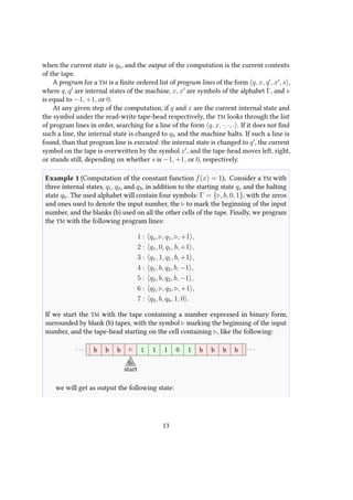
![b b b 1 b b b b b b b b
qh
end
. . .. . .
To see this, we have to analyse how the program given to the TM acts on the
initial tape: starting in the state qs on a tape cell with the symbol , the first line of
the program mandates the tape-head to move right and switch to the state q1. In
the q1 state, following the lines 2 and 3, the tape-head will move right over-writing
all the ones and zeros it finds, until it reaches a blank cell. When a blank cell is
reached, according to line 4, the tape-head changes its state to q2 and starts moving
left, continuing moving left, following line 5, until it reaches again the cell. When
the cell is reached, the state is changed to q3 and the tape-head is moved once on the
right. At this point, because of the line 7 of the program, the cell under the tape-head
- that is, the cell on the right of the one with - is over-written to 1, and the tape-head
state changed to qh, halting the execution.
The above analysis shows that this program computes the constant function
f(x) = 1. That is, regardless of what number is given in input onto the tape, the TM
halts with the number 1 represented onto the tape.
In general, a TM can be thought of as computing functions from the non-negative
integers to the non-negative integers, with the input to the function represented by the
initial state of the tape, and the output of the function by the final state of the tape.
The above presented TM is used to formalize the concept of a deterministic algorithm.
To also consider non-deterministic algorithms, this model must however be extended. For
this purpose, the TM model is generalized to that of a probabilistic TM. In a probabilistic
TM, the state transitions are choosen according to some probability distribution, instead
of being completely predetermined.
A further generalization of TMs provides a theoretical basis for quantum algorithms.
These are a special kind of algorithms which, exploiting the properties of quantum
mechanics, can potentially outperform any classical algorithm in certain tasks.
1.2 Church-Turing thesis
An interesting question is what class of functions is it possible to compute using a Turing
machine. Despite its apparent simplicity, the TM model can be used to simulate all
the operations performed on a modern computer. Indeed, according to a thesis put
forward independently by Church and Turing, the TM model completely captures the
notion of computing a function using an algorithm. This is known as the Church-Turing
thesis [28]:
14](https://image.slidesharecdn.com/51b2159f-4e1f-48f3-91cc-51dca4e8cf7b-160331120712/85/thesis-14-320.jpg)
![Church-Turing thesis: The class of functions computable by a Turing ma-
chine corresponds exactly to the class of functions which we would naturally
regard as being computable by an algorithm.
The Church-Turing thesis asserts an equivalence between the rigorous mathematical
concept of “function computable by a Turing machine”, and the intuitive concept of
what it means for a function to be computable by an algorithm. In this sense it is
nothing more than a definition of what we mean when we talk of the “computability” of
a function. This thesis is relevant because it makes the study of real-world algorithms
amenable to rigorous mathematical analysis.
We remark that it is not obvious that every function which we would intuitively
regard as computable by an algorithm can be computed using a TM. Indeed, it is conceiv-
able that in the future we will discover in Nature a process which computes a function
not computable by a TM. Up to now, however, no such process has been observed.
Indeed, as will be discussed in more detail in later sections, quantum computers also
obey the Church-Turing thesis. That is, quantum computers can compute the same
class of functions computable by a TM.
A much stronger statement than the Church-Turing thesis is the so-called Extended
Church-Turing thesis (ECT) [8] (also sometimes referred to as Strong Church-Turing
thesis [28]):
Extended Church-Turing thesis: All computational problems that are
efficiently solvable by realistic physical devices, are efficiently solvable by a
Turing machine.
The ECT was however already found to be insufficient to capture all realistic com-
putational models in the 1970s, when Solovay and Strassen [29] devised an efficient,
probabilistic primality test. As the Solovay-Strassen algorithm relied essentially on
randomness, it provided the first evidence that probabilistic Turing machines are capa-
ble to solve certain problems more efficiently than deterministic ones. This led to the
following ad-hoc modification to the ECT:
Extended Probabilistic Church-Turing thesis: All computational prob-
lems that are efficiently solvable by realistic physical devices, are efficiently
solvable by a probabilistic Turing machine.
As this is the form the ECT is currently usually stated as, this is the version we will refer
to when talking in the following of “ECT”.
However, even in this modified form, the ECT still does seem to be in contrast with
the currently accepted physical laws. The first evidence in this direction was given by
Shor [30], which proved that two very important problems - the problem of finding
the prime factors of an integer, and the so-called discrete logarithm problem - could
be solved efficiently on a quantum computer. Since no efficient classical algorithm -
neither deterministic nor probabilistic - is currently known to be able to efficiently solve
15](https://image.slidesharecdn.com/51b2159f-4e1f-48f3-91cc-51dca4e8cf7b-160331120712/85/thesis-15-320.jpg)
![these problems, Shor’s algorithm strongly suggests that quantum mechanics allows
to solve certain problems exponentially faster than any classical computer, and this
directly contradicts the ECT.
1.3 Complexity theory
Computational complexity theory analyzes the time and space resources required to
solve computational problems [28]. Generally speaking, the typical problem faced
in computational complexity theory is proving some lower bounds on the resources
required by the best possible algorithm for solving a problem, even if that algorithm is
not explicitly known.
One difficulty in formulating a theory of computational complexity is that different
computational models may lead to different resource requirements for the same problem.
For instance, multiple-tape TMs can solve many problems significantly faster than single-
tape TMs. On the other hand, the strong Church-Turing thesis states that any model of
computation can be simulated on a probabilistic TM with at most a polynomial increase
in the number of elementary operations required. This means that if we make the
coarse distinction between problems which can be solved using resources which are
bounded by a polynomial in n, and those whose resource requirements grow faster than
any polynomial in n, then this distinction will be well-defined and independent of the
considered computational model. This is the chief distinction made in computational
complexity.
With abuse of the term exponential, the algorithms with resource requirements
growing faster than any polynomial in n are said to require an amount of resources
scaling exponentially in the problem size. This includes function like nlog n
, which grow
faster than any polynomial but lower than a true exponential, and are nonetheless said
to be scaling exponentially, in this context. A problem is regarded as easy, tractable, or
feasible, if an algorithm for solving the problem using polynomial resources exists, and
as hard, intractable, or infeasible, if the best possible algorithm requires exponential
resources.
Many computational problems are formulated as decision problems, that is problems
with a yes or no answer. For example, the question is a given number m a prime number
or not? is a decision problem. Although most decision problems can easily be stated in
simple, familiar language, discussions of the general properties of decision problems are
greatly helped by the terminology of formal languages. In this terminology, a language
L over the alphabet Σ is a subset of the set Σ∗
of all finite strings of symbols from Σ.
For example, if Σ = {0, 1}, then the set of binary representations of even numbers
L = {0, 10, 100, 110, . . . } is a language over Σ. A language L is said to be decided by a
TM if for every possible input x ∈ Σ∗
, the TM is able to decide whether x belongs to
L or not. In other words, the language L is decided if the TM will eventually halt in a
16](https://image.slidesharecdn.com/51b2159f-4e1f-48f3-91cc-51dca4e8cf7b-160331120712/85/thesis-16-320.jpg)
![state encoding a “yes” answer if x ∈ L, and eventually halt to a state encoding a “no”
answer otherwise.
Decision problems are naturally encoded as problems about languages. For instance,
the primality decision problem can be encoded using the binary alphabet Σ = {0, 1},
interpreting strings from Σ∗
as non-negative integers, and defining the language L to
consist of all binary strings such that the corresponding number is prime. The primality
decision problem is then translated to the problem of finding a TM which decides the
language L. More generally, to each decision problem is associated a language L over
an alphabet Σ∗
, and the problem is translated to that of finding a TM which decides L.
To study the relations between computational problems, it is useful to classify them
into complexity classes, each one grouping all problems (that is, in the case of decision
problems, all languages) sharing some common properties. Most of computational
complexity theory is aimed at defining various complexity classes, and at understanding
of the relationships between different complexity classes.
A brief description of the most important complexity classes for decision problems
is provided in the following:
• P: We say that a given problem is in TIME(f(n)) if there is a deterministic TM
which decides whether a candidate x is in the corresponding language in time
O(f(n)), with n the length of x. A problem is said to be solvable in polynomial
time if it is in TIME(nk
) for some k. The collection of all languages which are in
TIME(nk
), for some k, is denoted P, which is an example of a complexity class
Some examples of problems in P are linear programming, the calculation of the
greatest common divisors of two numbers, and the problem of determining if a
number is prime or not.
Not surprisingly, there are lots of problems for which no polynomial-time algo-
rithm is known. Proving that a given decision problem is not in P, however, is very
difficult. A couple of examples of such problems are 1) given a non-deterministic
Turing machine M and an integer n written in binary, does M accept the empty
string in at most n steps? and 2) given a pair of regular expressions, do they represent
different sets?. Many other problems are believed to not be in P. Among these
are notable ones such as Factoring, which is the problem of finding the prime
factors decomposition of an integer. This problem is believed to hard problem for
classical computers, though no proof, nor compelling evidences for it, are known
to date. Factoring is particularly important, since its hardness lies at the heart
of wisely used algorithms in cryptography such as the RSA cryptosystem [28].
• NP: An interesting property of the prime factorization problem is that, even if
finding the prime factorization of an integer n is very hard, it is easy to check if a
proposed set of primes is indeed the correct factorization of n: just multiply the
numbers and check if they equal n. The class of decision problems sharing this
17](https://image.slidesharecdn.com/51b2159f-4e1f-48f3-91cc-51dca4e8cf7b-160331120712/85/thesis-17-320.jpg)
![property is called NP. More generally NP, standing for “nondeterministic poly-
nomial time”, is the class of all decision problems for which there are efficiently
verifiable proofs. A NP problem can often be intuitively stated in the form are
there any solutions that satisfy certain constraints?
While it is clear that P is a subset of NP, the converse is currently not known.
Indeed, whether P equals NP is arguably the most famous open problem in
computer science, often abbreviated as the P = NP problem. Many computer
scientists believe [31, 32, 33] that P = NP. However, despite decades of work,
nobody has been able to prove this, and the possibility that P = NP cannot be
excluded. Some implications of either of these possibilities are shown in fig. 1.1.
A related complexity class is NP-hard, which groups all decision problems that
are, informally, at least as hard as the hardest problems in NP. More precisely, a
problem L is NP-hard if every problem in NP can be reduced to L in polynomial
time. As a consequence, a polynomial algorithm solving an NP-hard would
also automatically provide a polynomial algorithm for all problems in NP. While
this is considered highly unlikely, as many NP problems are believed to not be
solvable in polynomial time, it has never been proved that this is not the case.
Finally, the intersection between NP and NP-hard is the class of the so-called
NP-complete problems.
• BPP: If we extend our definition of a TM allowing it to have access to a source of
randomness, let’s say the ability to flip a fair coin, other complexity classes can
be defined. Such a probabilistic Turing machine may only accept or reject inputs
with a certain probability, but if the probability of an incorrect accept or reject is
low enough, they are as useful as their deterministic counterparts. One of the
most important such classes is BPP, which stands for Bounded-error Probabilistic
Polynomial time. BPP is the class of decision problems solvable by a probabilistic
TM in polynomial time with a probability of error less than 1/3.
The choice of 1/3 as error bound is mostly arbitrary, as any error bound strictly
less than 1/2 can be reduced to practically zero with only a small increase in
the resource requirements. For this reason, problems in BPP are regarded as
as efficiently solvable as P problems. In fact, for practical purposes, BPP is
considered, even more than P, as the class of problems which are efficiently
solvable on a classical computer.
18](https://image.slidesharecdn.com/51b2159f-4e1f-48f3-91cc-51dca4e8cf7b-160331120712/85/thesis-18-320.jpg)
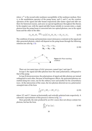
![Complexity
P ≠ NP P = NP
NP-Hard
NP-Complete
P
NP
NP-Hard
P = NP =
NP-Complete
Figure 1.1: Relations between the fundamental complexity classes.
All the above considered computational classes only took into account classical
Turing machines. The advent of quantum mechanics and the conception of quantum
computers, however, led to the question of what classes of problems can a quantum
computer solve? To try to answer this question, one must study another kind of
complexity classes, entering the realm of quantum complexity theory. In this context,
arguably the most fundamental complexity class if BQP, standing for Bounded-error
Quantum Polynomial time. This is the quantum generalization of BPP, and is defined
as the set of decision problems solvable by a quantum computer in polynomial time,
with an error probability of at most 1/3 for all instances. Probably the most notable
problem which has been shown to be in BQP is Factoring. Indeed, Shor’s algorithm
[30] was one of the first devised quantum algorithms able to efficiently solve a problem
that the best-known classical counterparts can solve only in exponential time.
While only decision problems have been mentioned to this point, these are not the
only kind of computational problems. Function problems are a generalized version of
decision problems, where the output of the algorithm is not bounded to be a simple
YES/NO answer. More formally, a function problem P is defined as a relation R over
the cartesian product over strings of an alphabet Σ, that is R ⊂ Σ∗
× Σ∗
. An algorithm
is said to solve P if for every pair (x, y) ∈ R, it produces y when given x as input.
A class of function problems that will be of interest in the following are the so-called
counting problems, which are problems that can be stated as how many X satisfy a certain
19](https://image.slidesharecdn.com/51b2159f-4e1f-48f3-91cc-51dca4e8cf7b-160331120712/85/thesis-19-320.jpg)
![property P? An example of such a complexity class is #P (pronounced “sharp P”), which
is the set of counting problems associated with the decision problems in NP. Intuitively,
to each NP problem which can be stated in the form “Are there any solutions having
the property P?” is associated a #P problem which can be stated in the form “How many
solutions are there which satisfy the property P?”. As can be intuitively deduced from
this definition, #P problems are generally believed to be even more difficult than NP
problems.
A pair of computational classes related to #P are #P-hard and #P-complete. These
are defined in a completely analogous way to NP-hard and NP-complete, containing
the class of counting problems at least as hard as any #P problem.
A notable instance of a #P-hard problem is the calculation of the permanent of a
complex-valued matrix. The permanent is a function of matrices defined similarly to
the determinant (see the discussions in the following sections, like definition 2), but
which, contrarily to the latter, is known to not be computable in polynomial time, for
general matrices [34]. Indeed, the problem of computing the permanent of a matrix is
known to be a #P-hard problem, and even #P-complete in special circumstances [34].
1.4 Quantum information and quantum computation
Quantum information theory [28, 35, 36, 37] is the study of the information processing
tasks that can be accomplished using quantum mechanical systems. One of the main
goals of quantum information theory is to investigate how information is stored in the
state of a quantum system, how does it differ from that stored in a classical system, and
how can this difference be exploited to build quantum devices with capabilities superior
to that of their classical counterparts. To this end several concepts and ideas are drawn
from other disciplines, such as quantum mechanics, computer science, information
theory, and cryptography, and merged with the goal of generalizing the concepts of
information and computing to the quantum realm.
In the last few decades, information and computation theory have undergone a
spurt of new growth, expanding to treat the intact transmission and processing of
quantum states, and the interaction of such quantum information with traditional forms
of information. We now know that a fully quantum theory of information offers, among
other benefits, a brand of cryptography whose security rests on fundamental physics,
and a reasonable hope of constructing quantum computers that could dramatically speed-
up the solution of certain mathematical problems. Moreover, at a more fundamental
level, it has become clear that an information theory based on quantum principles
extends and completes classical information theory, much like complex numbers extend
and complete the reals. One of the conceptual building blocks of quantum information
and quantum computation is that of a qubit. This is the quantum generalization of
the classical concept of bit, and the fundamental processing unit of most quantum
20](https://image.slidesharecdn.com/51b2159f-4e1f-48f3-91cc-51dca4e8cf7b-160331120712/85/thesis-20-320.jpg)
![devices. While a bit can be in one of two states, traditionally referred to as 0 and 1, a
qubit is allowed to be in a superposition of these basis states. Properly handling such
qubits, quantum computers are able to process information in ways impossible with
any classical computer.
The first to envisage the notion of a quantum computer was Feynman [1], as a
possible solution to the problem of the exponentially increasing amount of resources
required to simulate complex quantum systems with classical computers. More than a
decade later, Lloyd [38] showed that a quantum computer can indeed act as a universal
quantum simulator, where the word universal refers to the fact that the same machine
is capable of tackling vastly different problems by simply changing the program it runs.
There are a lot of candidate implementations for quantum computation. Among
these, in no particular order, are implementations using superconductors, trapped
ions, quantum dots, nuclear magnetic resonance, diamond nitrogen vacancies, silicon,
linear optics, and many other proposed technologies. Here we will only focus on linear
optical implementations of quantum computing, to highlight the difficulties inherent
to implement universal quantum computers, as opposite to the relatively much easier
demands of boson sampling devices, which will be described in the following sections.
Linear optics quantum computation (LOQC) with single photons has the advan-
tage that photons have very long decoherence times, which means that the quantum
information stored in photons tends to stay there, and that linear optical elements are
arguably the simplest building blocks to realize quantum information processing. The
downside is that photons do not naturally interact with each other, and in order to
apply two-qubit quantum gates, which are necessary to implement universal quantum
computation, such interactions are essential. Because of this, effective interactions
among photons have to be introduced somehow.
The two main methods to implement such interactions among photons are 1) using
Kerr nonlinearities, and 2) the use of projective measurements with photodetectors.
Unfortunately, present-day nonlinear Kerr media exhibit very poor efficiency [28] and
very weak nonlinearities, while projective measurements have the disadvantage of
producing probabilistic quantum gates: more often than not these gates fail, destroying
the quantum information.
In the case of projective-measurements-induced nonlinearities there is however
a way to avoid the issue of nondeterministic gates, still mantaning feasible resource
requirements: the Knill, Laflamme, and Milburn [7] (KLM) scheme. Introduced in 2001,
the KLM protocol allows scalable linear optics quantum computing by using quantum
gate teleportation to increase the probability of success of nondeterministic gates [7, 39,
40]. The downside of the KLM scheme is that, for its implementation, it is still necessary
to overcome a series of experimental challenges, such as the synchronization of pulses,
mode-matching, quickly controllable delay lines, tunable beam splitters and phase
shifters, single-photon sources, accurate, fast, single-photon detectors, and extremely
21](https://image.slidesharecdn.com/51b2159f-4e1f-48f3-91cc-51dca4e8cf7b-160331120712/85/thesis-21-320.jpg)
![fast feedback control of these detectors. While most of these features are not terribly
unrealistic to implement, the experimental state of the art is simply not at the point at
which more complex gate operations such as two-qubit operations can be implemented.
On the other hand, a quantum computer is not necessary to implement quantum
simulation. Dropping the requirement of being able to simulate any kind of system,
special purpose devices can be built to tackle specific problems better than the clas-
sical counterparts, in the simpler conceivable case by just emulating, in an analog
manner, the behaviour of a complex quantum system on a simpler quantum device.
Being generally these special purpose devices easier to implement than full-fledged
quantum computers, it is expected that practical quantum simulation will become a
reality well before quantum computers. However, despite the undeniable practical
usefullness of implementing quantum simulation on a classically intractable quantum
system, this would hardly give a definite answer to the question: are there tasks which
quantum computers can solve exponentially faster than any classical computer? Indeed,
a quantum system that is hard to classically simulate is also typically hard to define as
a computational problem. This makes extremely difficult to definitively prove whether
a classical algorithm, able to efficiently carry out such a simulation, exists.
It is for this reasons that the proposal of a boson computer by Aaronson and Arkhipov
[8] gained much interest in the quantum optics community. This kind of special purpose
linear optics quantum computer requires only to send n indistinguishable photons
through a random unitary evolution, and detect the output photons with standard
photodetectors. No teleportation or feedback mechanisms are required, which makes
the experimental implementation of such a device much easier than that of a quantum
computer following the KLM scheme. Furthermore, the related computational problem
is simple enough to be analytically tractable with the tools of computational complexity,
allowing to obtain very strong theoretical evidence of its hardness.
22](https://image.slidesharecdn.com/51b2159f-4e1f-48f3-91cc-51dca4e8cf7b-160331120712/85/thesis-22-320.jpg)
![sufficient to obtain the wave function at each time t: its solution is, at least formally,
given by |Ψ(t) = e−i(t−t0)H/
|Ψ(t0) .
The above described formalism is also called first-quantization, to distinguish it
from another way of dealing with quantum systems, named second-quantization. The
latter differs from the former by a shift in focus: instead of considering the number
of particles as a fixed property of the system and using the wave function to describe
their states, the system is characterized by the number of particles contained in each
possible mode, which are however no longer necessarily fixed. To this end, a creation
operator is defined, for each mode, as an operator which acts on a quantum state and
produces another quantum state differing from the former for a single quantum added
to that mode. The hermitian conjugate of a creation operator is called an annihilation
operator (also destruction operator), and instead of adding a quantum to a given mode,
it does the opposite, producing a new state with one less particle in the mode.
The exact rules followed by creation and annihilation operators depend on the
statistical nature of the particles. For bosons, the creation (annihilation) operator of a
mode labelled i is denoted ˆa†
i (ˆai). The core rules obeyed by these operators are the
following:
ˆai |ni =
√
n |(n − 1)i , ˆa†
i |ni =
√
n + 1 |(n + 1)i ,
[ˆak, ˆa†
q] = δk,q, [ˆak, ˆaq] = [ˆa†
k, ˆa†
q] = 0 ,
(2.3)
where |ni is a state with n particles in the mode labelled i. Quantum states with a
well-defined number of particles in each mode are called Fock states, or number states,
and the set of all Fock states is called Fock space.
The above defined creation operators can be used to denote many-boson states, that
is, quantum states with more than one indistinguishable boson. If any single boson can
be in one of m modes, an n-boson state r having ri particles in the i-th mode will be
written as
|r ≡ |r1, . . . , rm =
1
√
r!
m
k=1
ˆa†
k
rk
|0 . (2.4)
where the notation r! ≡ r1! · · · rk! has been used. Such a list r of m elements, with each
element equal to the number of particles in a given mode, will be referred to as the
Mode Occupation List (MOL) associated to the quantum state. A many-body state such
that for every k = 1, . . . , m, rk = 1 or rk = 0, is said to be a collision-free state.
Another way to characterize many-body states is through a so-called Mode Assign-
ment List (MAL) R . This is a list of n elements, with the i-th element being the mode
occupied by the i-th particle. It is worth noting that for indistinguishable particles one
cannot talk of “the mode of the i-th particle”, however. Because of this, the order of
the elements of MALs cannot have any physical significance. In other words, MALs are
always defined up to the order of the elements, or, equivalently, they must be always
considered conventionally sorted (for example, in increasing order). Representing the
24](https://image.slidesharecdn.com/51b2159f-4e1f-48f3-91cc-51dca4e8cf7b-160331120712/85/thesis-24-320.jpg)
![state with a MAL, eq. (2.4) can be rewritten in the following form:
|r ≡ |R =
1
√
r!
n
k=1
ˆa†
Rk
|0 =
1
µ(R)
n
k=1
ˆa†
Rk
|0 , (2.5)
where we denoted with µ(R) the product of the factorials of the occupation numbers
of the state R, that is, µ(R) ≡ r1! · · · rm!.
Yet another way to describe many-body states that will sometimes be useful is to
explicitly list the occupation numbers of each mode. For example, for a state with three
particles, one in the second mode and two in the fourth mode, we write |12, 24 . If
we want to emphasize the absence of particles in, say, the third mode, we write it as
|12, 03, 24 .
Definition 1 (MOL and MAL representations). All of the many-particle quantum
states used in the following will be assumed to have a fixed number of particles n,
with each particle potentially occupying one of m possible modes. Two ways to
represent a state are:
• As the Mode Occupation List (MOL) r ≡ (r1, . . . , rm), i.e. as the m-dimensional
vector whose element rk is the number of particles in the k-th mode. It follows
from this definition that m
k=1 rk = n. We will refer to this representation as
the MOL representation, and denote with Fn,m the set of all MOLs of n photons
into m modes, and with FCF
n,m the set of collision-free MOLs of n photons into
m modes:
Fn,m ≡ (r1, . . . , rm) | ∀i = 1, . . . , m, ri ≥ 0 and
m
i=1
ri = n , (2.6)
FCF
n,m ≡ {(r1, . . . , rm) ∈ Fn,m | ∀i = 1, . . . , m, ri ∈ {0, 1}} . (2.7)
• As the Mode Assignment List (MAL) R ≡ (R1, . . . , Rn), i.e. as the n-dimensional
vector listing the modes occupied by the particles. Given that for indistinguish-
able particles it is not meaningful to assign a specific mode to a specific particle,
the order of the elements of a MAL are conventionally taken to be in increas-
ing order, so to have a one-to-one correspondence between physical states
and MALs. We will refer to this representation as the MAL representation of a
many-particle quantum state and, following the notation of [41], denote with
Gn,m and Qn,m the set of all MALs of n photons into m modes and the set of
collision-free MALs of n photons into m modes, respectively. Equivalently, Gn,m
25](https://image.slidesharecdn.com/51b2159f-4e1f-48f3-91cc-51dca4e8cf7b-160331120712/85/thesis-25-320.jpg)
![Using eq. (2.5) into eq. (2.10) gives
|r
ˆU
−−−−→
1
√
r!
n
k=1
m
j=1
URk,j
ˆb†
j
|0 =
1
√
r!
m
j1=1
m
j2=1
· · ·
m
jn=1
n
k=1
URk,jk
ˆb†
jk
|0
=
1
√
r! ω∈Γn,m
n
k=1
URk,ω(k)
ˆb†
ω(k) |0 ,
(2.13)
where Γn,m is the set of all sequences of n positive integers lesser than or equal to m.
To compute the scattering amplitudes A(r → s, U) of going from the input r to the
output s ≡ (s1, . . . , sn), we now have to rearrange the terms on the right hand side of
eq. (2.13). To this end we start from the general combinatorial equation (see [41]):
ω∈Γn,m
f(ω1, . . . , ωn) =
ω∈Gn,m
1
µ(ω) σ∈Sn
f(ωσ(1), . . . , ωσ(n)), (2.14)
where f(ω) ≡ f(ω1, . . . , ωn) is any function of n integer numbers, Gn,m is the sequence
of all non-decreasing sequences of n positive integers lesser than or equal to m, given
in definition 1, and Sn is the symmetric group, that is, the set of permutations of n
elements.
Applying eq. (2.14) to eq. (2.13), with f(ω1, . . . , ωn) = n
k=1 URkωk
ˆb†
ωk
, we obtain
|r
ˆU
−−−−→
1
µ(R) ω∈Gn,m
1
µ(ω) σ∈Sn
n
k=1
URk,ωσ(k)
ˆb†
ωσ(k)
|0
=
ω∈Gn,m
1
µ(R)µ(ω)
σ∈Sn
n
k=1
URk,ωσ(k)
|ω1, . . . , ωn out ,
(2.15)
where in the last step we exploited the commutativity of the product of the creation
operators ˆb†
k.
We thus obtained the following expression for the scattering amplitudes for bosonic
particles:
A(r → s, U) ≡ out s|r ≡ s| ˆU |r =
1
µ(R)µ(S)
σ∈Sn
n
k=1
URk,Sσ(k)
, (2.16)
in which the factor on the right hand side can be recognised as the permanent of an
appropriate matrix built from U.
28](https://image.slidesharecdn.com/51b2159f-4e1f-48f3-91cc-51dca4e8cf7b-160331120712/85/thesis-28-320.jpg)
![Definition 2 (Permanent). The permanent of a square matrix, similarly to the de-
terminant, is a function which associates a number to a matrix. It is defined very
similarly to the determinant, with the exception that all minus signs that are present
for the latter become plus signs in the former.
More precisely, the permanent of a squared n×n matrix A = (aij) is
perm(A) =
σ∈Sn
a1,σ(1) · · · an,σ(n) =
σ∈Sn
n
k=1
ak,σ(k), (2.17)
where Sn is the symmetric group, that is, the set of all permutations of n distinct
objects.
To express eq. (2.16) through the above defined permanent function, it is also useful
to introduce the following notations to refer to particular submatrices built from a given
matrix:
Definition 3. Let Mk,l denote the set of all k×l complex-valued matrices. If k = l
we shall write Mk instead of Mk,k. Now, let A ∈ Mk,l, and let α ∈ Gp,k and β ∈ Gq,l.
Then, we shall denote with A[α|β] the p × q dimensional matrix with elements
A[α|β]i,j ≡ Aαi,βj
. If, moreover, α ∈ Qp,k and β ∈ Qq,l, then A[α|β] is a submatrix
of A. If α = β we will simplify the notation to write A[α] instead of A[α|β].
Again, if α ∈ Qp,k and β ∈ Qq,l, we shall denote with A(α|β) the (k − p)×(l − q)
dimensional submatrix of A complementary to A[α|β], that is, the submatrix obtained
from A by deleting rows α and columns β.
Example 4. Consider the 3×4 dimensional matrix A =
1 2 3 0
4 5 6 i
0 4 2 1
. Then, if
α = (1, 1) ∈ G2,4 and β = (2, 4, 4) ∈ G3,3, we have A[α|β] ≡
2 0 0
2 0 0
. If
instead α = (2, 3) ∈ Q2,4 and β = (1, 2) ∈ Q2,3, we have A[α|β] ≡
4 5
0 4
and
A(α|β) ≡ 3 0 .
Using definitions 2 and 3, we see that for any matrix A ∈ Mm and sequences
α, β ∈ Gn,m, we have
perm(A[α|β]) =
σ∈Sn
n
k=1
Aαk,βσ(k)
,
29](https://image.slidesharecdn.com/51b2159f-4e1f-48f3-91cc-51dca4e8cf7b-160331120712/85/thesis-29-320.jpg)
![which is just the factor in brackets on the right hand side of eq. (2.16). We conclude that
A(r → s, U) ≡ out s|r ≡ s| ˆU |r =
1
µ(R)µ(S)
perm(U[R|S]). (2.18)
It is worth noting that the symmetric nature of the bosonic creation operators - that
is, the fact that [ˆa†
i , ˆa†
j] = δij - was essential in the above derivation. Analogous
reasonings carried out using fermionic particles - whose creation operators satisfy
{ˆc†
i , ˆc†
j} ≡ c†
i c†
j + c†
jc†
i = δij - would lead to the result
Afermions
(r → s, U) = det(U[R|S]). (2.19)
While eqs. (2.18) and (2.19) may seem very similar at first glance, especially given
the similarities in the definitions of permanents and determinants, they are extremely
different when trying to actually compute these scattering amplitudes. Indeed, while
the determinant of an n dimensional matrix can be efficiently computed, the same is
in general not true for permanents. This is exactly what makes the BosonSampling
problem interesting, and will be described in detail in the next sections.
In conclusion, we can now write down the unitary matrix describing the evolution
of the many-body states, that is, the matrix Uα,β(m, n, U), with α, β ∈ Gn,m, whose
elements contain the permanents (or the determinants, in the case of fermions) of the
corresponding matrix given by eq. (2.18):
Uα,β(m, n, U) ≡
1
µ(α)µ(β)
perm(U[α|β]), α, β ∈ Gn,m. (2.20)
The dependence of U on n, m, and U will often be omitted when clear from the context.
Example 5. Consider the 3×3 unitary matrix Ui,j ≡ ui,j, injected with 2-photon
input states. The resulting many-boson scattering matrix is:
U(3, 2, U) =
u2,3u3,2 + u2,2u3,3 u2,3u3,1 + u2,1u3,3 u2,2u3,1 + u2,1u3,2
√
2u2,3u3,3
√
2u2,2u3,2
√
2u2,1u3,1
u1,3u3,2 + u1,2u3,3 u1,3u3,1 + u1,1u3,3 u1,2u3,1 + u1,1u3,2
√
2u1,3u3,3
√
2u1,2u3,2
√
2u1,1u3,1
u1,3u2,2 + u1,2u2,3 u1,3u2,1 + u1,1u2,3 u1,2u2,1 + u1,1u2,2
√
2u1,3u2,3
√
2u1,2u2,2
√
2u1,1u2,1√
2u3,2u3,3
√
2u3,1u3,3
√
2u3,1u3,2 u2
3,3 u2
3,2 u2
3,1√
2u2,2u2,3
√
2u2,1u2,3
√
2u2,1u2,2 u2
2,3 u2
2,2 u2
2,1√
2u1,2u1,3
√
2u1,1u1,3
√
2u1,1u1,2 u2
1,3 u2
1,2 u2
1,1
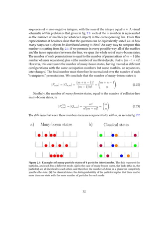
2.2 Counting many-body states
Another interesting property of many-body states is their number. Unlike classical
states, it is not meaningful to assign a state to the single particles of a quantum many-
body state. A quantum state is instead described only giving the list of modes occupied
30](https://image.slidesharecdn.com/51b2159f-4e1f-48f3-91cc-51dca4e8cf7b-160331120712/85/thesis-30-320.jpg)
![2.3.4 Single-photon sources
An ideal single-photon source [42, 43, 44] would be one that
1. Is deterministic (or “on demand”), meaning that it can emit a single photon at any
arbitrary time defined by the user,
2. Has a 100% probability of emitting a single photon and a 0% probability of multiple-
photon emission,
3. Subsequently emitted photons are indistinguishable,
4. The repetition rate is arbitrarily fast.
Given however that no real-world photon source satisfies all of these specifications,
the deviations from the ideal characteristics must be considered when designing exper-
iments.
Single-photon sources are broadly classified into deterministic and probabilistic.
Among the implementations of the former are those based on color centers [45, 46, 47],
quantum dots [48, 49, 50], single atoms [51], single ions [52], single molecules [53],
and atomic ensembles [54], all of which can to some degree emit single photons “on
demand”. On the other hand are the probabilistic single-photon sources. These generally
rely on photons created in pairs via parametric downconversion in bulk crystals and
waveguides, and four-wave mixing in optical fibers. While these sources are probabilistic
- and therefore it is not possible to know exactly when a photon has been emitted -
because the photons are created in pairs, one of the emitted photons can be used to
herald the creation of the other.
While the distinction between deterministic and probabilistic sources is clear in the
abstract, this distinction blurs in practice. This due to the unavoidable experimental
errors that make also “theoretically deterministic sources” be probabilistic in practice.
Although many applications, especially those in the field of quantum-information
science, require an on-demand source of single photons, probabilistic single-photon
sources remain a fundamental tool, and are widely used in many quantum optics
experiments.
Spontaneous parametric downconversion (SPDC) is an important process in quan-
tum optics, typically exploited to generate entangled photon pairs, or heralded single
photons. This is achieved using a nonlinear crystal - that is, a medium in which the
dielectric polarization responds nonlinearly to the electric field - which converts the
photons of a pump beam into pairs of photons of lower energy. A simple model of the
interaction Hamiltonian in such a crystal is
HI ∼ χ(2)
ˆapˆa†
sˆa†
i + hermitian conjugate, (2.36)
37](https://image.slidesharecdn.com/51b2159f-4e1f-48f3-91cc-51dca4e8cf7b-160331120712/85/thesis-37-320.jpg)
![with |pi = (ˆa†
i )p
/
√
p!, and 0 ≤ g < 1 an appropriate parameter determining the ratio
of generated photons and dependent, among other things, on the strength of the pump
beam. Typically, g 1, so that the probability of generating many photons is low. For
instance, in typical conditions g ∼ 0.1 and the probability of generating a state of the
form |21 |22 is lower of a factor ∼ 102
than the probability of producing a single pair
|11 |12 .
The main advantages of SPDC sources are the high photon indistinguishability, the
collection efficiency, and relatively simple experimental setups. This technique, however,
suffers from two drawbacks. First, since the nonlinear process is nondeterministic, so is
the photon generation, even though it can be heralded. Second, the laser pump power,
and hence the source’s brilliance, has to be kept low to prevent undesired higher-order
terms in the photon generation process.
Figure 2.6: Representation of type II downconversion. The pump beam (red) impinges on the nonlinear
crystal, generating, due to birefringence effects, photons along two cones. On the upper ordinary cone
(orange), the generated photons are horizontally polarized, while on the lower extraordinary cone (green)
the generated photons are vertically aligned. Postselecting on the two intersections of these cones (blue
dots), a pair of polarization-entangled photons is obtained.
2.3.5 Single-photon detectors
Roughly speaking, single-photon detectors are devices which convert single photons
into an electrical signal of some sort [42]. Quantum information science is one of the
field currently driving much of the research toward improved single-photon-detector
technology. For example, many quantum communication protocols rely heavily on
39](https://image.slidesharecdn.com/51b2159f-4e1f-48f3-91cc-51dca4e8cf7b-160331120712/85/thesis-39-320.jpg)
![detector properties such as detection efficiency.
An ideal single-photon detector [42] would require the following characteristics:
1. The detection efficiency - that is, the probability that a photon incident upon the
detector is successfully detected - is 100%,
2. The dark-count rate - that is, the rate of detector output pulses in the absence of
any incident photons - is zero,
3. The dead time - that is, the time after a photon-detection event during which the
detector is incapable of detecting another photon - is zero,
4. The timing jitter - that is, the variation from event to event in the delay between
the input of the optical signal and the output of the electrical signal - is zero.
Additionally, an ideal single-photon detector would also be able to count the number of
photons in an incident pulse. Detectors able to do this are referred to as photon-counting,
or photon-number resolving, detectors. However, non-photon-number-resolving detec-
tors, which can only distinguish between zero photons and more than zero photons,
are the most commonly used. Indeed, while detecting a single photon is a difficult task,
discriminating the number of incident photons is even more difficult. Examples of non-
photon-number-resolving single-photon detector technologies include single-photon
avalanche photodiodes [55], quantum dots [56], superconducting nanowires [57], and
up-conversion detectors [58, 59, 60].
2.4 Hong-Ou-Mandel effect
The differences between bosons and fermions are not only in the different numbers of
microstates. Their statistical behaviour can differ significantly, as well as be significantly
different from the behaviour of distinguishable particles.
Bosons, roughly speaking, tend to occupy the same state more often than classical
particles, or fermions, do. This behaviour, referred to as bosonic bunching, has been
verified in numerous experimental circumstances, including fundamental ones like
Bose-Einstein condensation [61, 62, 63]. In the context of optical experiments, the most
known effects arising from the symmetric nature of the Bose-Einstein statistics is the
Hong-Ou-Mandel (HOM) effect [64].
In the original experiment, two photons are sent simultaneously through the two
input ports of a symmetric beam splitter. Since no interaction between the two photons
takes place, one would expect no correlation between the detection events at the two
output ports. Instead, the photons are always seen either both on the first output mode,
or both on the second output mode.
40](https://image.slidesharecdn.com/51b2159f-4e1f-48f3-91cc-51dca4e8cf7b-160331120712/85/thesis-40-320.jpg)
![+ − +
Figure 2.7: Pictorial representation of the suppression of non-bunched events, when two indistinguish-
able bosons evolve through a symmetric beam splitter. Each of the four images represent a possible
evolution of the bosons, with all of them interfering with each other. The two events which would result
in one boson per output port turn out to interfere destructively (note the minus sign), and are suppressed.
This effect is a direct consequence of the quantum interference between the possible
ways two-photon states can evolve. A pictorial representation of this is given in fig. 2.7:
when the photons are injected into two different ports of a symmetric beam splitter,
the scattering amplitudes corresponding to the output photons being in two different
modes interfere destructively.
We can derive this result applying eq. (2.33) to the two-photon input state |11, 12 =
ˆa†
1ˆa†
2 |0 :
|11, 12 = ˆa†
1ˆa†
2 |0 →
1
√
2
ˆb†
1 − iˆb†
2
1
√
2
−iˆb†
1 + ˆb†
2 |0
=
1
2
−i(ˆb†
1)2
+ ˆb†
1
ˆb†
2 − ˆb†
2
ˆb†
1 − i(ˆb†
2)2
=
−i
2
(ˆb†
1)2
+ (ˆb†
2)2
|0 =
−i
√
2
(|21 + |22 ) ,
(2.41)
where in the last steps we used the rules given in eq. (2.3), and in particular the
commutativity of the bosonic creation operators, which implies that ˆb†
1
ˆb†
2 = ˆb†
2
ˆb†
1 (see
also fig. 2.7 for a pictorial representation of how the suppression of non-bunched events
arises). We thus conclude that when two indistinguishable photons enter a symmetric
beam splitter one in each mode, they always come out in the same mode.
This property of photons (or, more generally, of bosons) is highly non-classical, and
is a notable example of how interesting effects can arise when dealing with many-body
quantum states.
In a real world experiment, the two input photons will never be perfectly indistin-
guishable, though. A more careful analysis, taking into account the potentially different
times at which the photons reach the beam splitter, as well as the coherence time of
each photon wave packet, predicts a smooth transition from the classical behaviour to
the antibunching effect described above [65].
In the general case of partially distinguishable particles, the probability PT (s, x) of
detecting an output state s in an HOM experiment with a time delay quantified by x,
becomes an average of the probability PB for bosons and the probability PD assigned
to distinguishable particles, weighted by two factors |c1|2
and |c2|2
which depend on
41](https://image.slidesharecdn.com/51b2159f-4e1f-48f3-91cc-51dca4e8cf7b-160331120712/85/thesis-41-320.jpg)
![the relative time delay:
PT (s, x) = |c1(x)|2
PB(s) + |c2(x)|2
PD(s). (2.42)
In a typical experimental scenario, with the incoming photons having a Gaussian
frequency distribution around the central frequency, PT (s, x) also has a gaussian profile
[65], as shown in a typical case in fig. 2.8.
In the case of fully distinguishable particles, where PT = PD, no interaction
occurs and the output events of the single photons are not correlated. There are
two possible classical configurations of two photons in the output MOL (1, 1), and
one configuration for both (2, 0) and (0, 2). It follows that PD((1, 1)) = 2/4 and
PD((2, 0)) = PD((0, 2)) = 1/4, as shown in fig. 2.8 for x ≈ ±400µm. On the other
hand, when the particles are fully indistinguishable, PT = PB. The probability of the
various outcomes is now given by eq. (2.41). The output (1, 1) is thus suppressed, while
PB((2, 0)) = PB((0, 2)) = 1/2, as shown in fig. 2.8 for x = 0.
Figure 2.8: Transition to indistinguishability in a HOM experiment. Changing the time delay between
the two input photons a dip in the number of measured output coincidences is seen, corresponding
to the time delay (or, equivalently, the path delay) making the photons indistinguishable. The blue
line is the probability of detecting two photons in one of the two output ports, that is, PT ((2, 0), x) or
equivalently PT ((0, 2), x). The red line is the probability PT ((1, 1), x) of detecting the two photons in
the two different output ports. As expected, the red plot shows a peak corresponding to the antibunching
effect arising when the particles are indistinguishable, while the blue plot show the HOM explained above.
42](https://image.slidesharecdn.com/51b2159f-4e1f-48f3-91cc-51dca4e8cf7b-160331120712/85/thesis-42-320.jpg)
![Chapter 3
BosonSampling
In this chapter we discuss various aspects of the BosonSampling computational prob-
lem. In section 3.1 the problem of experimentally assessing quantum supremacy is
discussed, in order to appreciate the importance of BosonSampling in the modern
research context. Section 3.2 follows with the description of what the BosonSampling
computational problem is, and its advantages in obtaining experimental evidences
of quantum supremacy. In section 3.3 some issues related to the scalability of boson
sampling implementations are described. The chapter closes with a description of
scattershot boson sampling in section 3.4, as an alternative architecture to scale boson
sampling implementations to higher numbers of photons.
3.1 Importance of BosonSampling
It is currently believed that many quantum mechanical systems cannot be efficiently
simulated with a classical computer [1]. This implies that a quantum device is, to the
best of our knowledge, able to solve problems de facto beyond the capabilities of classical
computers. Exploiting this quantum advantage requires however an high degree of
control over the quantum system, not yet manageable with state of the art technology.
In particular, a post-classical computation with a universal quantum computer will
require an high degree of control of a large number of qubits, and this implies that an
experimental evidence of quantum supremacy [3] with an universal quantum computer
will likely require many years. A notable example is given by the large gap between the
number of qubits that can currently be coherently controlled (∼10), and the number
of qubits required for a calculation such as prime factorization, on a scale that would
challenge classical computers (∼106
). Consequently, there is considerable interest in
non-universal quantum computers and quantum simulators that, while able to only
solve specific problems, might be significantly easier to be implemented experimentally.
Such devices could give the first experimental demonstration of the power of quantum
43](https://image.slidesharecdn.com/51b2159f-4e1f-48f3-91cc-51dca4e8cf7b-160331120712/85/thesis-43-320.jpg)
![devices over classical computers, and potentially lead to technologically significant
applications.
Moreover, in the context of searching for experimental evidence of quantum supremacy,
the technological difficulties are not the only issue. To show this, we will consider as an
example Shor’s quantum algorithm [30] to efficiently factorize integer numbers. Even if
we were to get past the technological difficulties of implementing Shor’s algorithm with
sufficiently many qubits, it could be easily argued that such an achievement would not
be a conclusive evidence that quantum mechanics allows post-classical computations.
This because we do not have to date a mathematically sound proof that there cannot be a
classical algorithm to efficiently factorize integers. In the language of complexity theory,
this corresponds to the fact that we do not have a proof that Factoring is not in P,
even though this is believed enough to base modern cryptography is based on this
conjecture. More generally, before 2010, there were no instances of problems efficiently
solved by quantum computers, which were proved to not be efficiently solvable with
classical ones.
This changed when, in 2010, Aaronson and Arkhipov (AA) proposed [8] the Boson-
Sampling problem as a way to obtain an easier experimental evidence of quantum
supremacy. BosonSampling is a computational problem that, while hard to solve for
a classical computer, is efficiently solved by a special-purpose quantum device. AA
showed that BosonSampling is naturally implemented using only linear optical ele-
ments, in a photonic platform named a boson sampler. The experimental realization
of a boson sampler, while still challenging with present-day technologies, requires
much less experimental efforts with respect to those required to build a universal
quantum computer. In fact, the AA scheme requires only linear optical elements and
photon-counting detectors, as opposite to, for example, the Knill, Laflamme & Milburn
approach [7, 40] for universal linear optics quantum computing, which requires among
other things an extremely fast feedback control of the detectors.
44](https://image.slidesharecdn.com/51b2159f-4e1f-48f3-91cc-51dca4e8cf7b-160331120712/85/thesis-44-320.jpg)
![Figure 3.1: Galton board: n identical balls are dropped one by one from the upper corner, and are
randomly scattered into the lower slots. The quantum generalization of this classical “rudimentary
computer” leads to the idea of BosonSampling. Credits: Nicolò Spagnolo.
3.2 The BosonSampling computational problem
Consider the following linear optical experiment: the n-photon state |rAA given by
|rAA ≡ |11, . . . , 1n, 0n+1, . . . , 0m ≡ ˆa†
1 . . . ˆa†
n |01, . . . , 0m , (3.1)
is injected into a passive linear optics network, which implements a unitary map on
the creation operators:
ˆa†
k → ˆUˆb†
k
ˆU†
=
m
j=1
Uk,j
ˆb†
j. (3.2)
with U an Haar-random m×m complex unitary matrix. The evolution induced on
|rAA is
|rAA →
s∈Fn,m
A(r → s, U) |s , (3.3)
where the sum is extended over all many-boson states of n particles into m modes, and
the scattering amplitudes A are, as shown in eq. (2.18), proportional to the permanents
of n×n matrices. AA argued that, for m n, the output of such an apparatus cannot
be efficiently predicted by a classical computer, neither exactly nor approximately [8].
This was rigorously proved in the exact case. The problem of approximately sampling
45](https://image.slidesharecdn.com/51b2159f-4e1f-48f3-91cc-51dca4e8cf7b-160331120712/85/thesis-45-320.jpg)
![from the output probability distribution of a boson sampling apparatus depends instead
on a series of conjectures, for which strong supporting evidence was provided [8].
This problem, which amounts to that of being able to sample from the output proba-
bility distribution given in eq. (2.18), is referred to as the BosonSampling computational
problem. The constraint m n is essential for the hardness result, as otherwise
semi-classical methods become efficient [66, 67].
Roughly speaking, a boson sampling apparatus is a “quantum version” of a Galton
board. A Galton board, named after the English scientist Sir Francis Galton, is an
upright board with evenly spaced pegs into its upper half, and a number of evenly-
spaced rectangular slots in the lower half (see fig. 3.1). This setup can be imagined to
be a rudimentary “computer”, where n identical balls are dropped one by one from
the upper corner, and are randomly scattered into the lower slots. In the quantum
mechanical version, the n balls are indistinguishable bosons “dropped” simultaneously,
and each peg a unitary transformation, typically implemented as a set of beam splitters
and phase shifters.
More precisely, BosonSampling consists in producing a fair sample of the output
probability distribution P(s |U, rAA) ≡ |A(r → s, U)|2
, where s is an output state of
the n bosons, and rAA the above mentioned input state. The unitary ˆU and the input
state rAA are the input of the BosonSampling problem, while a number of output states
sampled from the correct probability distribution are its solution (see fig. 3.2).
46](https://image.slidesharecdn.com/51b2159f-4e1f-48f3-91cc-51dca4e8cf7b-160331120712/85/thesis-46-320.jpg)
![Figure 3.2: Conceptual boson sampling apparatus. (a) The input of the BosonSampling problem is
the input many-photon state (in figure the state |0, 0, 1, 1, 0, 1, 0, 0, 0 ), and a suitably chosen unitary U.
The output is a number of outcomes picked according to the bosonic output probability distribution (in
figure, two examples of such states are provided, with MOLs 101000100 and 110000100). Colleting enough
such events allows to reconstruct the probability distribution. This, however, requires an exponentially
increasing (in n) number of events. (b) Injecting an m-mode unitary with n indistinguishable photons,
the output state is a weighted superposition of all possible outcomes. Measuring in which modes the
photons ended up results in the collapsing of this superposition. The probability of finding the photons
in a certain configuration is given by eq. (3.4). Credits: [10].
47](https://image.slidesharecdn.com/51b2159f-4e1f-48f3-91cc-51dca4e8cf7b-160331120712/85/thesis-47-320.jpg)
![from the correct probability distribution would theoretically be enough to achieve
a post-classical computation, though possibly making it harder to experimentally
verify.
The hardness of the BosonSampling problem can be traced back to the #P-hardness
of computing the permanent of a generic complex-valued matrix. Indeed, as shown in
eq. (2.18), the probability P(r → s, U) of an input r evolving into s, is proportional to
the permanent of the matrix U[R|S] (recalling definition 3):
P(r → s, U) = |A(r → s, U)|2
=
1
µ(R)µ(S)
|perm(U[R|S])|2
. (3.4)
Computing the permanent of a n×n matrix with the fastest known classical algorithms
[41, 68] requires a number of operations of the order O(n2n
). This means that, for
example, computing the permanent of a 30×30 complex matrix, corresponding to a
single scattering amplitude for a 30-photon state, requires a number of operations of the
order of ∼ 1010
. If the average time required by a classical computer to perform a single
operation is of the order ∼ 107
, the computation of one such scattering amplitude
will require ∼ 10 minutes. While still clearly manageable by a classical computer,
this already shows the potential advantages of a boson sampling apparatus: if the
experimental problems related to coherently evolve 30 indistinguishable photons inside
an interferometer were to be solved, this would allow to sample from the probability
distribution given by eq. (3.4) without actually knowing the probabilities itselves.
AA demonstrated that, should boson sampling be classically easy to solve, this would
have very strong and undesied consequences in computational complexity theory, and
therefore it is most probable that boson sampling is not classically easy to solve.
It is worth stressing that the BosonSampling problem is not that of finding the per-
manents in eq. (2.18), but only that of sampling from the related probability distribution.
In fact, not even a boson sampler is able to efficiently compute these scattering probabil-
ities. This is due to the fact that, to reconstruct a probability distribution spanning over
a number M of events, roughly speaking, the number of samples is required to be at
least of the order of M. But, as shown in eqs. (2.22) and (2.23), M scales exponentially
with n, implying that the number of experimental samples required to reconstruct the
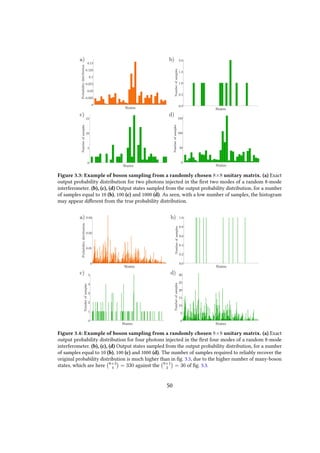
probability distribution becomes exceedingly large very soon. In figs. 3.3 and 3.4 is
shown that, if the number of samples is not large enough, the reconstructed probability
distribution is different from the real one. In fact, generally speaking, there are strong
arguments against the possibility to compute the permanents of complex-valued matri-
ces by means of quantum experiments [69], although attempts have been reported in
this direction [70].
49](https://image.slidesharecdn.com/51b2159f-4e1f-48f3-91cc-51dca4e8cf7b-160331120712/85/thesis-49-320.jpg)
![The complexity of BosonSampling makes it an extremely valuable candidate to gain
experimental evidences of the supremacy of quantum devices over classical computers.
Indeed, it presents several advantages in this regard over, for example, Factoring,
which is the paradigmatic problem that would allow quantum computers to perform a
post-classical computation:
1. The BosonSampling problem is even harder than Factoring, being related to
the #P-hard complexity class, and believed to not be in NP.
2. A boson sampler requires significantly less resources to be implemented than a
universal quantum computer. In particular, it does not require adaptive or feed-
forward mechanisms, nor fault-tolerance methods. This relatively simple design
has already prompted a number of small-scale implementations of increasing
complexity [9, 10, 11, 12, 13, 14, 15, 17, 18, 25, 71].
AA suggested [8] that a 400-modes interferometer fed with 20 single photons
is already at the boundary of the simulation powers of present-day classical
computers. While in this regime it would still be possible to carry out a classical
simulation, the quantum device should be able to perform the sampling task faster
than the classical computer.
3. The theoretical evidence of the hardness of BosonSampling is stronger than that
of factoring integers: while in the former case the result only relies on a small
number of conjectures regarding the hardness of some problems [8], in the latter
case there is no compelling evidence for Factoring to not be in P. While known to
be in BQP, Factoring is only believed to be in NP, and strongly believed to not
be in NP-hard.
While the hardness of Factoring is strong enough to build modern cryptography,
it could also happen that a polynomial-time algorithm will be discovered showing
that Factoring is in P as, basically, the sole evidence for its hardness is the fact
that no efficient classical algorithm is yet known.
3.3 Scaling experimental boson sampling implemen-
tations
The hardness of BosonSampling has another potentially important consequence: it
could provide the first experimental evidence against the ECT [8]. This point, however,
is still subject to some debate [67, 72, 73], due to the somewhat informal nature of
the ECT itself. Indeed, the ECT is not a mathematical statement, but a statement about
how the physical world behaves, in a certain asymptotic limit. Because of this it is
51](https://image.slidesharecdn.com/51b2159f-4e1f-48f3-91cc-51dca4e8cf7b-160331120712/85/thesis-51-320.jpg)
![somewhat ill-defined what exactly would be “enough experimental evidence” to “prove”
or “disprove” such a statement.
While AA argued for the hardness of both the exact and approximate BosonSam-
pling problems, they did not take into account other forms of experimental imperfec-
tions.
More precisely, AA showed that even attempting to estimate the output probability
distribution of a boson-sampler is likely computationally hard, as long as the probability
P of each input state being correctly produced by the sources scales as P > 1/ poly(n),
that is, does not vanish faster than the inverse of a polynomial in n [8]. Further evidence
that even lossy systems or systems with mode mismatch are likely to be classically hard
to solve was later given [74].
Another source of errors which could potentially undermine the scalability of boson
sampling are the unavoidable circuit imperfections, especially taking into account
the fact that a boson sampler cannot likely implement fault-tolerant mechanisms [8].
Therefore, small errors in the calibrations of the elementary optical elements, like
beam splitters and phase-shifters, may accumulate and result in an output probability
distribution significantly different from the ideal one. A thorough analysis of this issue,
reported in [75], leads to the result that as long as the average fidelity of the elementary
gates scales at least like 1 − O(1/n2
), the overall implementation provides a reasonably
good output distribution.
Generally speaking, all of these works seem to reinforce the idea that the Boson-
Sampling problem is scalable even when experimentally plausible conditions are taken
into account. This however, is not definitively enstablished. While the potential for
scaling up the number of modes of network implementations has been fairly well
enstablished, and experiments with 2 photons into up to 21 modes have been reported
[76], scaling the number of photons is much harder and will likely require technologi-
cally improvements, especially on the side of the employed single-photon sources and
detectors.
In particular, most reported boson sampling experiments used SPDC single-photon
sources. With this type of scheme, using a single SPDC source, the probability of
producing n photons decreases exponentially with n, as shown in eq. (2.40). This
means that in order to implement a boson sampler with higher numbers of photons
another kind of architecture is most likely required. One such example is provided by a
scattershot boson sampler, which will be described in the next section.
3.4 Scattershot boson sampling
One of the main difficulties in scaling up the complexity of boson sampling devices is
the requirement of a reliable source of many indistinguishable photons. Indeed, despite
recent advances in photon generation [42] using atoms, molecules, color centers in
52](https://image.slidesharecdn.com/51b2159f-4e1f-48f3-91cc-51dca4e8cf7b-160331120712/85/thesis-52-320.jpg)
![diamond, and quantum dots, currently the most widely used method remains parametric
downconversion. The drawbacks of SPDC sources, described in section 2.3.4, have
however restricted SPDC implementations of boson sampling experiments to proof-of-
principle demonstrations.
Recently a new scheme, named scattershot boson sampling [19], has been proposed
to make the best use of SPDC sources for photonic boson sampling, greatly enchancing
the rate of n-photon events [19, 20]. As opposite to a boson sampling experiment, in
which a single fixed input state is employed, in a scattershot boson sampler the photons
are injected into randomly chosen modes at each shot. This is achieved adopting
an heralded single-photon source for every mode of the interferometer (see fig. 3.5).
If a single source has a probability p of injecting a photon into the interferometer
for each laser pulse, the probability of n particular sources injecting a photon at the
same time is pn
. However, there are m
n
possible combinations of sources that can
simultaneously inject a photon into the interferometer, so that the resulting probability
of injection of any configuration of n photons is m
n
pn
. For m n2
, which is the
regime in which BosonSampling is hard, the binomial factors dominate over pn
. Thus,
while the efficiency of using a single SPDC source to generate many photons decreses
exponentially with pn
, the overall efficiency of a scattershot boson sampling apparatus
with m SPDC sources increases exponentially with n, in the regime n m, as shown in
fig. 3.6.
While a scattershot boson sampling apparatus would technically solve a problem
different from BosonSampling as defined above, due to the randomly changing input
state, it has been shown [19, 20] that the computational problem solved by a scattershot
boson sampler is at least as hard as BosonSampling, thus making this new scheme as
good as the original one to achieve a post-classical computation.
An experimental implementation of a scattershot boson sampler has been recently
reported [18], using a 13-mode integrated photonic chip and up to six SPDC sources, to
obtain data corresponding to two- and three-photon interference.
53](https://image.slidesharecdn.com/51b2159f-4e1f-48f3-91cc-51dca4e8cf7b-160331120712/85/thesis-53-320.jpg)
![Figure 3.5: A scattershot boson sampler. An SPDC source is used for every input of the m-mode
interferometer. Each SPDC source generates (ignoring higher order terms) a pair of photons, one of
which is injected into the interferometer, while the other heralds the generation event. Every time a
detector corresponding to an heralding photon “clicks”, we know that a photon has been injected into
the corresponding mode of the interferometer. (image courtesy of [18])
m =8
m =16
m =32
m =64
0 10 20 30 40 50 60
n
100
106
1010
1014
1018
p =0.5
p =0.1
p =0.01
5 10 15 20 25 30
n
1010
1020
1030
1040
1050
11
a) b)
Figure 3.6: (a) Logarithmic plot of the binomial factor m
n as a function of n, for m equal to 8 (blue), 16
(orange), 32 (green) and 64 (red). (b) Logarithmic plot of the probability pn n2
n of injecting n photons
into an m = n2
-modes interferometer with a scattershot boson sampling apparatus, against the number
of photons n, with the single pair generation probability p equal to 0.01 (blue), 0.1 (orange) and 0.5
(green). The plot shows how the probability increases exponentially with n. Moreover, the lower is the
value of p, the higher is the number of photons required to see this advantage, as seen here in the case of
p = 0.01. Credits: [18].
54](https://image.slidesharecdn.com/51b2159f-4e1f-48f3-91cc-51dca4e8cf7b-160331120712/85/thesis-54-320.jpg)
![Chapter 4
Boson sampling validation
In this chapter we discuss the problem of validating boson sampling experiments.
In section 4.1 the problem is presented in its generality. In section 4.2 we focus on
the validation protocols based on zero-transmission laws. A validation scheme with
Fourier matrices is described, an experimental implementation of which is given in
chapter 6. In section 4.3 we discuss the possibility of validating scattershot boson
sampling experiments with the above described validation scheme for Fourier matrices.
In section 4.4 an alternative validation scheme, based on Sylvester matrices, is presented.
The advantages of this protocol to validate scattershot boson sampling experiments is
discussed.
4.1 Validating boson sampling implementations
The very hardness of BosonSampling, while being its main feature, also poses the
problem of certifying the results of an experimental implementation. This means that
if someone were to present an alleged boson sampling device as a black box, we may
not be able to certify its output. In other words, we may not be able to tell if the output
of the black box is the result of true many-body interference, as opposite, say, of that
of a classical computer giving in output a series of randomly chosen samples. From
a complexity-theoretical point of view, this is due to the fact that BosonSampling
belongs to the #P class [8], and thus not classically verifiable in polynomial time.
More intuitively, we can trace back the causes of this certification problem to two
fundamental factors:
Hardness of computing the bosonic probability distribution: It is not possible
to efficiently calculate with classical resources, and probably neither with quantum
ones [8], the bosonic output probability distribution. While this may naively be thought
of as the main issue, it does not imply per se a fundamental certification problem. As a
counterexample we may think of Factoring: while it is not (as to the current state of
55](https://image.slidesharecdn.com/51b2159f-4e1f-48f3-91cc-51dca4e8cf7b-160331120712/85/thesis-55-320.jpg)
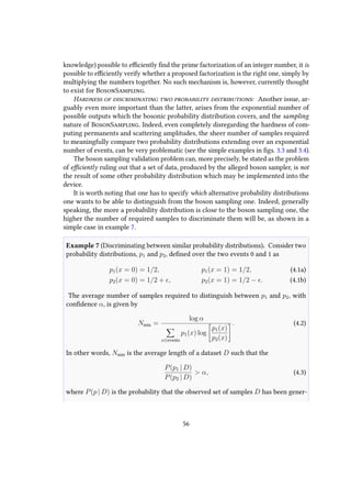
![ated by the probability distribution p. Applying eq. (4.2) to eq. (4.1) we obtain
Nmin ≈
log α
2 2
+ O(1), for → 0. (4.4)
Thus as expected, decreasing , and thus increasing the “similarity” of the two distri-
butions, the number of required samples increases indefinitely.
From the experimental point of view, this poses the very concrete issue of finding
a way to certify that a built experimental apparatus is working as aspected. From a
more fundamental standpoint instead, an unsolved validation problem threatens to
crucially undermine the theoretical claim of observing a post-classical computation:
if we are given by an untrusted party an alleged boson sampler as a black box, which
efficiently produces a number of samples faster than any classical computer can sample
from the boson sampling distribution, how can we somehow certify that that output is
what it claims to be? Indeed, an issue may arise if the number of samples necessary
to assess that the produced set of data does not come from an alternative probability
distribution increases exponentially with n, thus making an experimental, verifiable
implementation of the BosonSampling problem not scalable.
When the boson sampling validation problem was first raised, it was argued to
be fundamentally unsolvable, thus undermining the possibility of experimentally dis-
criminate a boson sampling distribution even against the trivial uniform one [77].
AA subsequently showed that this was not true, providing an example of an efficient
method to discriminate the boson sampling distribution from the uniform one [21].
This test, however, was not capable of efficiently separating, for example, the output
of a boson sampler from that resulting from the evolution of classical particles into
the interferometer. This validation test was successfully implemented in a number of
experiments [14, 15].
Other tests, able to validate against distinguishable particles, were later proposed
[14, 15, 16, 21, 22, 23] and experimentally implemented [14, 15, 17].
4.2 Fourier suppression law
Among the proposed validation schemes, those based on Zero-Transmission Laws (ZTLs)
[24] (also often referred to as suppression laws) seem to be a promising approach to
discriminate true many-boson evolution from alternative models. A ZTL can be thought
of as a generalization of the HOM effect to many modes and photons. More precisely,
it refers to the capability, occurring in some particular unitary matrices, to efficiently
predict the strict suppression of certain input-output combinations of states. In other
words, a ZTL allows to efficiently predict that for certain pairs of states (r, s), the
scattering amplitude A(r, s) vanishes, without having to compute a permanent.
57](https://image.slidesharecdn.com/51b2159f-4e1f-48f3-91cc-51dca4e8cf7b-160331120712/85/thesis-57-320.jpg)
![Such suppressions, like the HOM effect, are a pure quantum-mechanical effect, arising
from the interference of many-body states during the evolution in the interferometer,
and as such a strong signature of non-classical evolution.
In the originally proposed BosonSampling scheme, where a random unitary matrix
is employed, no such ZTL can be taken advantage of. However, these turn out to be
useful when thinking to the validation problem in a slightly broader perspective. If
we do not think of a boson sampler as a black box, but approach the more practical
problem of assessing that an actual experimental apparatus is working as advertised,
we can analyse the various possible sources of error. Roughly speaking, the two main
factors potentially leading to an erroneous output probability distribution are: a wrong
implemented unitary evolution, and non-indistinguishable input states. While the
unitary matrix implemented in an interferometer can be efficiently verified [78], the
indistinguishability of the input photons is harder to assess, and it is in this context
that ZTLs can be exploited.
Provided that one can change at will the unitary matrix implemented in the device -
which is in principle possible to do efficiently [79] and has been recently reported in an
experimental setup [17] - then it is possible to first verify the indistinguishability of
the sources by injecting the photons in a specially crafted unitary, whose symmetries
allow to efficiently observe a ZTL, and then on the same device to implement a random
unitary matrix and perform the boson sampling experiment.
The first proposed example of such a ZTL [24] employed Fourier matrices:
Definition 4 (Fourier matrices). Let UF
(m) be the m-dimensional matrix defined
element-wise by
[UF
(m)]j,k ≡
1
√
m
exp
2πi
m
(j − 1)(k − 1) , j, k = 1, . . . , m. (4.5)
We will refer in the following to this matrix as the m×m Fourier matrix. The m
dependence will be omitted when clear from the context.
It was shown [22, 24, 65, 66] that with Fourier matrices, a b-periodic input state r
never evolves in an output state s such that b n
j=1 Sj is not a multiple of the number
of modes m, where S is the MAL introduced in definition 1, and a b-periodic state is
defined as follows:
Definition 5 (Periodic states). Given a state r, we say that r is b-periodic if its MOL
representation has the form
r ≡ (r1, . . . , rb, r1, . . . , rb, . . . , r1, . . . , rb)
m=p·b
, (4.6)
58](https://image.slidesharecdn.com/51b2159f-4e1f-48f3-91cc-51dca4e8cf7b-160331120712/85/thesis-58-320.jpg)
![√
2 UF
(2) =
1 1
1 −1
√
3 UF
(3) =
1 1 1
1 e
2πi
3 e
−2πi
3
1 e
−2πi
3 e
2πi
3
√
4 UF
(4) =
1 1 1 1
1 i −1 −i
1 −1 1 −1
1 −i −1 i
Table 4.1: Examples of Fourier matrices
where b is the length of each of the identical sublist (bins) composing r, and p = m/b
the number of such sublists. We will refer to b as the periodicity of r.
Being UF
symmetric, that is, UF
i,j = UF
j,i for every i and j, the scattering amplitudes
are also symmetric with respect to input and output states: A(r → s, UF
) = A(s →
r, UF
). In conclusion, the Fourier suppression law [24] can be stated as follows:
Theorem 1 (Fourier suppression law). Let UF
(m) be the m×m Fourier matrix, and
let r and s be two n-boson states, with corresponding MAL representations R and S.
Then, if r is b-periodic and s is such that
mod
b
n
j=1
Rj, m
= 0, (4.7)
then the following suppression law holds:
A(r → s, UF
) = A(s → r, UF
) = 0. (4.8)
We note that the converse in in general not true. In other words, this condition is
sufficient but not necessary for an input-output pair to be suppressed.
The many-boson matrices corresponding to Fourier matrices with m = 4, 6, 8, and
n = 2, are shown in figs. 4.1 to 4.3. In these figures, the periodic states are highlighted in
green, and the strictly suppressed states are the white squares. The input-output pairs
predicted to be suppressed by theorem 1 are marked by purple circles. The majority
of the suppressed pairs correspond to periodic states, and are predicted by theorem 1.
Figure 4.3 shows however that theorem 1 gives a sufficient but not necessary condition
for a pair to be suppressed, as there are in this case pairs which are suppressed but do
not correspond to periodic states.
59](https://image.slidesharecdn.com/51b2159f-4e1f-48f3-91cc-51dca4e8cf7b-160331120712/85/thesis-59-320.jpg)
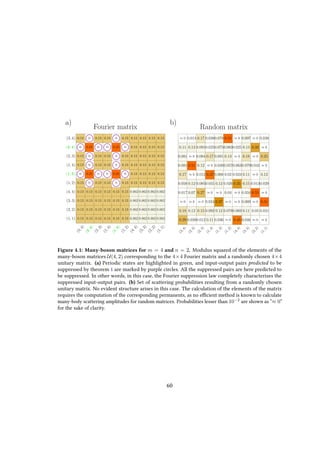
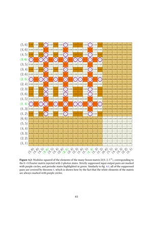
![The validation scheme which exploits the Fourier suppression law, proposed in [22],
uses a single fixed input state with MAL
RTichy = (1, np−1
+ 1, 2np−1
+ 1, . . . , (n − 1)np−1
+ 1), (4.9)
injected into an inteferometer implementing the m-dimensional Fourier matrix, with
m = np
and p some positive integer. RTichy is an especially crafted n-periodic state,
corresponding to an high fraction of output suppressed states. Counting the number
of states corresponding to a suppressed input-output pair - that is, an input-output
pair that would be suppressed if the evolution was an ideal quantum-mechanical one - it
is possible to quantify how much the observed output probability distribution differs
from the ideal boson sampling one.
More precisely, the violation parameter is defined as
D = Nforbidden/Nruns, (4.10)
where Nforbidden is the number of observed events violating theorem 1, and Nruns is the
total number of events. This parameter has been shown [22] to be a better signature
of quantum many-body statistics than precedently proposed validation schemes. In
particular, it can be used to validate a boson sampler against alternative hypotheses
such as the Mean-Field Sampler [22]. A Mean-Field Sampler is an efficiently evaluable
and physically plausible alternative model [22], which reproduces some aspects of
many-boson dynamics surviving in the semiclassical limit. This model is not distin-
guished from the boson sampler distribution by other validation schemes, making the
Fourier validation test more capable of capturing the signatures of genuine many-boson
quantum interference. A summary of the validation protocol based on Fourier matrices
is given in fig. 4.4.
63](https://image.slidesharecdn.com/51b2159f-4e1f-48f3-91cc-51dca4e8cf7b-160331120712/85/thesis-63-320.jpg)
![Figure 4.4: Validation scheme with Fourier matrices. Conceptual scheme of the protocol: the
possible configurations of n photons at the output of an m-mode interferometer can be divided into
two categories, unforbidden and forbidden, depending on whether they satisfy or not the suppression
confition of theorem 1, respectively. The pie charts show the expected output statistics with different
classes of particles, where green and red areas represent events with unforbidden and forbidden outputs,
respectively. The injection of a cyclic Fock state (beige box) in an m-mode Fourier interferometer results
in total suppression of forbidden output states. Cyclic states with distinguishable particles (blue box) show
no suppression, being each output combination equally likely to occur. A Mean Field state [22] (purple
box), a semi-classical state reproducing some of the features of bosonic statistics, shows suppression
with highly reduced contrast. Therefore, with a cyclic input the m-mode Fourier interferometer is able
to discriminate, through the measurement of degree of violation D = Nforbidden/Nevents, which of these
three hypotheses the input state belongs to. Credits: [25].
64](https://image.slidesharecdn.com/51b2159f-4e1f-48f3-91cc-51dca4e8cf7b-160331120712/85/thesis-64-320.jpg)
![4.3 Fourier suppression law and scattershot boson sam-
pling
The original scheme for implementing a boson sampler using a single SPDC source is not
scalable to higher number of photons, as discussed in the earlier sections. Scattershot
boson sampling is, currently, the most promising architecture to implement Boson-
Sampling with higher number of photons. This scheme, however, is essentially based
on the injection of random input states into the interferometer. On the other hand,
the validation scheme based on the Fourier suppression law only works for particular,
periodic input states. Therefore, a scattershot boson sampling experiment cannot be
validated making use of the Fourier suppression law, as originally proposed.
For a validation scheme based on some ZTL to be employable with a scattershot
boson sampler, it is no more sufficient to have an high number of output suppressed
states corresponding to some small class of input states. Instead, it is required that the
fraction of pairs of suppressed input-output states must be a non-negligible fraction
of the total number of states. In other words, considering that all input states in a
scattershot boson sampler are collision-free, and approximating all output states to also
be collision-free (which is justified in the m n limit [80]), we must have
suppressed input-output configurations
m
n
2 > 0 by a statistically significant amount.
(4.11)
In this section we consider whether this condition is verified for the Fourier sup-
pression law, thus making it viable to use in scattershot boson sampling experiments.
We will proceed by counting how many input states have some kind of periodicity,
according to eq. (4.6), and are thus such that theorem 1 can be applied to them. For the
same reasons given above, we will restrict our analysis to the collision-free states.
To count the number N(m, n) of periodic collision-free configurations (periodic
CFCs) of n photons in m modes, we first need to know for which values of b there can
be b-periodic configurations, given m and n. In other words, we want all the integers b
such that the MOL corresponding to the state can be written in the form (4.6).
Given that a partition of the MOL of the form (4.6) can be found for each p = 1
which is a common divisor of m and n, we have that the possible b are all and only the
integers of the form b = m/p for such a p. Formally, we say that the set B(m, n) of all
possible bin lengths b for n photons in m modes is
B(m, n) = {b ∈ N | b = m/p for some p = 1 common divisor of m and n}. (4.12)
Denoting with S(m, n, b) the set of all m-modes, n-photons, b-periodic CFCs, we
65](https://image.slidesharecdn.com/51b2159f-4e1f-48f3-91cc-51dca4e8cf7b-160331120712/85/thesis-65-320.jpg)
![1000 2000 3000 4000
n
200
400
600
800
1000
1200
1400
Figure 4.6: Logarithm of the number of periodic states
of m/2 photons in m modes, plotted as a function of m.
The coloured dashed lines are, in descending slope order,
log m/2
m/4
, log m/3
m/6
, log m/5
m/10
, log m/7
m/14
.
5 10 15 20 25 30 35
n
5
10
15
20
25
30
35
10 20 30 40
n
1000
2000
3000
4000
5000
6000
7000
10 20 30 40 50
n
1×10⁶
2×10⁶
3×10⁶
4×10⁶
5×10⁶
Figure 4.7: Number of periodic states vs number of photons. Blue points: number of periodic
states calculated with eq. (4.16). The continuous green, cyan, purple and red lines are respectively m/2
n/2
,
m/3
n/3
, m/5
n/5
and m/7
n/7
.
Unlike the number of periodic collision-free configurations, an efficient algorithm to
compute the number of suppressed output states predicted by Tichy’s suppression law
for Fourier matrices has not been found yet, except for very particular input states [22].
A brute force computation of the number of suppressed output states for each input
state for various values of m and n is shown in figs. 4.8 and 4.9. These computations
show that only a small fraction of input states results in a significant fraction of output
suppressed states.
However, the above result regarding the number of periodic states is enough to
make the Fourier suppression law unsuitable to validate scattershot boson sampling
experiments. In fact, in the best case scenario in which n = 2p
for some p, the number
of periodic states is ≈ m/2
n/2
(see eq. (4.20)), which is negligibly small compared to m
n
.
In particular, for m = n2
, the fraction n2/2
n/2
/ n2
n
decreases exponentially with n. This
implies that, even if all of these input states were to correspond to an 100% fraction of
output suppressed states, which is far from true, nevertheless in the regime of high n
virtually no suppressed pair would ever be sampled in a actual scattershot experiment,
and the validation scheme would be inefficient.
68](https://image.slidesharecdn.com/51b2159f-4e1f-48f3-91cc-51dca4e8cf7b-160331120712/85/thesis-68-320.jpg)
![5 10 15 20 25
0
20
40
60
80
Inputs
%ofsuppressedstates
8 modes, 2 photons
0 20 40 60 80 100 120
0
20
40
60
80
Inputs
%ofsuppressedstates
16 modes, 2 photons
0 10 20 30 40 50 60 70
0
20
40
60
80
Inputs
%ofsuppressedstates
8 modes, 4 photons
0 500 1000 1500
0
20
40
60
80
Inputs
%ofsuppressedstates
16 modes, 4 photons
5 10 15 20 25
0
20
40
60
80
Inputs
%ofsuppressedstates
8 modes, 6 photons
0 2000 4000 6000 8000
0
20
40
60
80
Inputs
%ofsuppressedstates
16 modes, 6 photons
a) b)
c) d)
e) f)
Figure 4.8: Ratio of suppressed collision-free output states For each input collision-free state, the
percentage of output suppressed collision-free states is shown for Fourier matrices (blue dots) and
Sylvester matrices (red dots). All the points are calculated using eq. (3.4). In all the cases shown the
number of suppressed output states is significantly higher for the Sylvester matrix. (a) and (b): For
two input photons, all of the output suppressed states are predicted by theorems 1 and 2 in the case of
Fourier and Sylvester matrices, respectively. Green dashed line: exact fraction of suppressions predicted
by eq. (4.24). (c) and (d): For n = 2p
only a subset of suppressed pairs are predicted by theorems 1
and 2. Green dashed line: estimate of the fraction of output suppression states, equal to 1 − 1/n. The
approximation gets closer to the true value for large values of n and m. (e) and (f): For n not equal to a
power of 2, no estimate of the number of output suppressed states is given, neither in [22] nor in [23].
69](https://image.slidesharecdn.com/51b2159f-4e1f-48f3-91cc-51dca4e8cf7b-160331120712/85/thesis-69-320.jpg)
![0 1000 2000 3000 4000
0
20
40
60
80
Inputs
%ofsuppressedstates
16 modes, 5 photons
0 2000 4000 6000 8000 10 000 12 000
0
20
40
60
80
Inputs
%ofsuppressedstates
16 modes, 8 photons
a) b)
Figure 4.9: Ratio of suppressed collision-free output states for each input in a 16-mode interferometer
injected with 5 (a) and 8 (b) photons. Like fig. 4.8, the ratio of suppressed output states is significantly
higher for almost all input states for the Sylvester matrix than the Fourier matrix.
4.4 Sylvester suppression law
Besides the Fourier matrix, a ZTL has been shown to exist also for another important
class of unitary matrices [23], the so-called Sylvester matrices.
Definition 6 (Sylvester matrices). Let US
be an m-dimensional unitary matrix of
the form US
(m) ≡ H(m)/
√
m, with H(m) defined recursively as
H(2p
) =
H(2p−1
) H(2p−1
)
H(2p−1
) −H(2p−1
)
, (4.21)
for each positive integer p, and with H(1) = 1. We will refer in the following
to US
(m) as normalized Sylvester matrix and to H(m) as Sylvester matrix. The m
dependence of US
and H will be omitted when clear from the context.
An analytic expression for the element (i, j) of a Sylvester matrix can be given in
the form:
[H(2p
)]i,j = (−1)iB jB
, (4.22)
where iB and jB are the binary representations of i and j, with rows and columns
enumerated from zero to m − 1, and is the bitwise dot product. For example, for
m = 8, i = 2, j = 7 we would have
[H(8)]2,7 = (−1)(0,1,0)·(1,1,0)
= (−1)0×1+1×1+0×0
= −1. (4.23)
70](https://image.slidesharecdn.com/51b2159f-4e1f-48f3-91cc-51dca4e8cf7b-160331120712/85/thesis-70-320.jpg)
![H(2) =
1 1
1 −1
H(4) =
1 1 1 1
1 −1 1 −1
1 1 −1 −1
1 −1 −1 1
H(8) =
1 1 1 1 1 1 1 1
1 −1 1 −1 1 −1 1 −1
1 1 −1 −1 1 1 −1 −1
1 −1 −1 1 1 −1 −1 1
1 1 1 1 −1 −1 −1 −1
1 −1 1 −1 −1 1 −1 1
1 1 −1 −1 −1 −1 1 1
1 −1 −1 1 −1 1 1 −1
Table 4.2: Examples of Sylvester matrices
We will refer in the following to US
(m) as normalized Sylvester matrix and to H(m) as
Sylvester matrix. The m dependence of US
and H will be omitted when clear from the
context.
It was recently proved [23] that injecting two bosons into any pair of (different)
modes of a multi-mode interferometer implementing a Sylvester matrix, the total
fraction of suppressed output states is
Nsupp
Ntot
= m
2(m+1)
. Considering only collision-free
states, the fraction becomes
Nsupp
Ntot,CF
=
m
2(m − 1)
. (4.24)
More generally, the following suppression law holds [23]:
Theorem 2 (Sylvester suppression law). Given an m×m Sylvester matrix, m = 2p
,
n = 2q
, q < p, and an n-boson input state with MAL S of the form
S = (1 + nc, . . . , n + nc), (4.25)
for some integer c such that 0 ≤ c ≤ (m/n − 1), then the strictly suppressed output
states are all and only those R ≡ (R1, R2, . . . , Rn) such that
R1,B ⊕ · · · ⊕ Rn,B = 0 ≡ (0, . . . , 0
q
), (4.26)
where Ri,B is the q-dimensional vector obtained from the binary representation of
Ri − 1 truncated to the q least significant digits, and ⊕ is the bitwise XOR operation
(equivalently the elementwise, modulo 2, sum).
Similarly to the case of Fourier matrices, an estimate of the fraction of strictly
suppressed states predicted by this law is:
V =
Nsupp
Ntot
≈ 1 −
1
n
. (4.27)
71](https://image.slidesharecdn.com/51b2159f-4e1f-48f3-91cc-51dca4e8cf7b-160331120712/85/thesis-71-320.jpg)
![Theorem 2 predicts an high ratio of suppressed output configurations for all input states,
when n = 2, as also shown in the numerical computations in figs. 4.8 and 4.9, and in the
many-boson matrices shown in figs. 4.10 and 4.11 On the other hand, this suppression
law predicts in the general case of n > 2 photons an high ratio of suppressed output
configurations only for the m/n input states of the form (4.25). This is a negligibly small
fraction of the total number of m
n
collision-free configurations, apparently making
Sylvester matrices even worse than Fourier matrices to validate a scattershot boson
sampler.
However, a brute force computation with eq. (2.18) shows (see figs. 4.8 and 4.9)
that the number of suppressed input-output pairs in a Sylvester matrix is significantly
higher than what predicted by the above described suppression law.
As will be showed in the following chapter, it is however possible to efficiently
predict a greater number of suppressed pairs, by generalizing the ZTL proposed in [23].
72](https://image.slidesharecdn.com/51b2159f-4e1f-48f3-91cc-51dca4e8cf7b-160331120712/85/thesis-72-320.jpg)
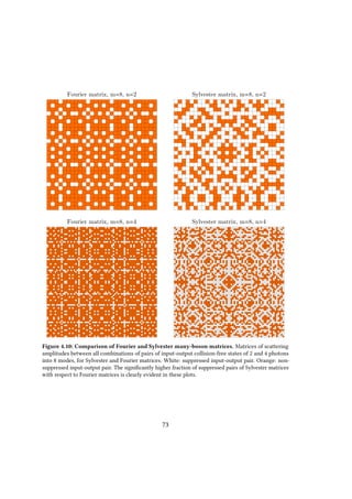
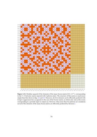
![Chapter 5
Theoretical results
As discussed in section 4.4, the suppression law given in theorem 2 [23] is not suitable
to validate scattershot boson sampling experiments. On the other hand, as shown
in figs. 4.8 and 4.9, the actual fraction of suppressed pairs is significanly higher, and
some kind of suppression law seems to hold for every input state, not just for those
considered by theorem 2.
In this chapter we propose a generalization of theorem 2, which predicts a much
higher fraction of suppressed pairs, and is thus more suitable to validate scattershot
boson sampling experiments. The proposed suppression law is described in section 5.2,
using notations and lemmas given in section 5.1. In section 5.3 we discuss a validation
scheme to distinguish quantum many-boson interference (up to small errors) from the
output resulting from distinguishable photons, by exploiting the proposed suppression
law. In this context we also derive an analytic expression for the mean number of
samples necessary to experimentally distinguish a nearly quantum evolution from the
classical hypothesis. The chapter closes with a summary of the results in section 5.4.
5.1 Preliminaries
For the results presented in this chapter we will introduce some new notations, on top of
those given in definition 1:
Definition 7 (Binary Matrix representation). Let r = (r1, . . . , rm) be the MOL
of a state of n particles in m = 2p
modes, for some positive integer p, and let
R = (R1, . . . , Rn) be the corresponding MAL. We denote with R
(2)
i the binary repre-
sentation of Ri − 1, padded with zeros on the left so as to make it a vector of length
p, and with Ri,α the α-th element of R
(2)
i . This construction allows us to represent
a many-body state r as a binary matrix (BM) R, i.e. as an n×p-dimensional matrix
75](https://image.slidesharecdn.com/51b2159f-4e1f-48f3-91cc-51dca4e8cf7b-160331120712/85/thesis-75-320.jpg)
![whose elements are either 0 or 1. We will refer to R as the BM representation (or
simply the BM) of the state r.
Remark 1. We note that for indistinguishable particles it is not meaningful to assign
a specific mode to a particle. This means that the order of the elements of the MAL
describing a state of many indistinguishable particles is not relevant. In other words, if
two MALs R and R differ only for the order of their elements, they represent the same
physical state. Similarly, if two binary matrices R and R can be obtained one from the
other with only a reordering of the rows, they represent the same physical state.
Example 8. Consider the case m = 4 and n = 2, and the state with MOL r ≡
(0, 1, 1, 0) and corresponding MAL R = (2, 3). Following the notations introduced
above we will have R1 = (0, 1), R2 = (1, 0), and the BM of r will be the 2×2 matrix
R =
0 1
1 0
.
Example 9. Consider the case m = 8, n = 4, and the state with MOL
s ≡ (1, 1, 1, 0, 0, 0, 0, 1) and corresponding MAL S = (1, 2, 3, 8). Following the no-
tations introduced above we will have S1 = (0, 0, 0), S2 = (0, 0, 1), S3 = (0, 1, 0),
S4 = (1, 1, 1), and the BM representation of r will be the 4×3 matrix
S =
0 0 0
0 0 1
0 1 0
1 1 1
.
Definition 8. Let R be an n×p BM, and let A be a subset of the p columns of R. Then
we denote with NA
(R) the matrix obtained by negating the columns of R specified
in A. In other words, expliciting the indices, NA
(R) is defined as
[NA
(R)]k,α ≡
Rk,α ⊕ 1, for α ∈ A,
Rk,α, for α /∈ A.
(5.1)
where ⊕ is the sum modulo 2.
Similarly, if r is a MOL representing some state of m = 2p
modes, we denote with
NA
(r) the MOL obtained applying to r the following three operations:
• Convert r to the binary matrix R,
76](https://image.slidesharecdn.com/51b2159f-4e1f-48f3-91cc-51dca4e8cf7b-160331120712/85/thesis-76-320.jpg)
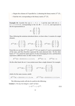
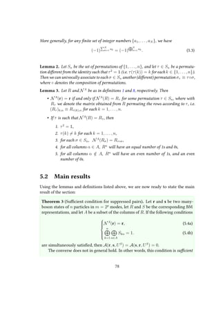
![but not necessary for a pair to be suppressed.
Proof. From now on, we will use the abbreviation A ≡ A(r, s, US
), leaving implicit
the dependence on the states and the unitary evolution considered. The transition
amplitude A can be expressed in terms of a permanent of the form
A =
1
√
r1! . . . rm!s1! . . . sm!
perm US
[R|S] , (5.5)
where perm(U) denotes the permanent of U, and the notation US
[R|S] was given in
definition 3.
Using definition 6 and eq. (4.22), we get from eq. (5.5)
A = C
σ∈Sn
n
k=1
(−1)Rσ(k) Sk
= C
σ∈Sn
(−1)ER,S(σ)
, (5.6)
where we denoted with Rσ(k) Sk the bitwise dot product between Rσ(k) and Sk, defined
as Rσ(k) Sk ≡ p
α=1 Rσ(k),αSk,α, C is a constant factor, and we defined the expression
at the exponent of the last expression (see lemma 1) as
ER,S(σ) ≡
n
k=1
Rσ(k) Sk =
n
k=1
p
α=1
Rσ(k),αSk,α. (5.7)
In the following, we will omit for brevity the dependence of the exponent E from the
states and write the above expression as simply E(σ). Note that the actual value of
E(σ) is not important here: the only relevant detail is its parity.
Since we need to evaluate only the cancellation of the scattering amplitude A,
we will ignore the constant factor C and focus on the sum over the permutations in
eq. (5.6). For this sum to vanish, it is necessary and sufficient that for exactly half of
the permutations we have (−1)E(σ)
= 1. In other words, the scattering amplitude A
vanishes if and only if the number of permutations σ such that E(σ) is even, is equal
to the number of permutations σ such that E(σ ) is odd. A necessary and sufficient
condition for this to hold, is that to each permutation σ we can univocally associate
another different permutation σ such that E(σ ) = 1 ⊕ E(σ).
But if eq. (5.4a) holds, then by lemma 3 and lemma 2 we can univocally associate
to each σ the (different) permutation στ ≡ τ ◦ σ, where τ is a permutation such that
NA
(R) = Rτ . Using στ in eq. (5.7) we have
E(στ ) =
n
k=1
p
α=1
Rτ(σ(k)),αSk,α =
n
k=1
α∈A
Rτ(σ(k)),αSk,α ⊕
α/∈A
Rτ(σ(k)),αSk,α
.
(5.8)
79](https://image.slidesharecdn.com/51b2159f-4e1f-48f3-91cc-51dca4e8cf7b-160331120712/85/thesis-79-320.jpg)
![Using now the explicit expression for NA
(R) given in definition 8 and the last result of
lemma 3, we have
NA
(Rσ) = Rτ◦σ ⇐⇒
1 ⊕ Rσ(k),α = Rτ(σ(k)),α, α ∈ A,
Rσ(k),α = Rτ(σ(k)),α, α /∈ A.
(5.9)
Inserting these equations in (5.8), we finally obtain
E(στ ) = E(σ) ⊕
n
k=1 α∈A
Sk,α = E(σ) ⊕ 1, (5.10)
where in the last step we exploited eq. (5.4b) for S. Inserting this last result into eq. (5.6)
we conclude that
A = C
σ∈Sn
(−1)ER,S(σ)
= C
σ∈Sn: E(σ) even
(−1)E(σ)
+ (−1)E(στ )
= 0, (5.11)
which proves that the input/output pair (r, s) is suppressed.
Example 11. Let r be the MOL given in example 10. Then NA
(r) = r holds for
A = {2}, A = {3}. and A = {2, 3}. Theorem 3 predicts that all output states s,
which BM representation S has an odd number of 1s in the second or third column,
are suppressed. Moreover, all output states with BM S having a total number of 1s in
the second and third column, are suppressed. More explicitly, all output states s such
that
n
k=1
Sk,2 = 1 or
n
k=1
Sk,3 = 1 or
n
k=1
[Sk,2 ⊕ Sk,3] = 1,
are predicted to be suppressed. For example, the states S = (3, 6, 7, 8), S = (2, 6, 7, 8),
and S = (4, 6, 7, 8), having BM representations
0 1 0
1 0 1
1 1 0
1 1 1
,
0 0 1
1 0 1
1 1 0
1 1 1
, and
0 1 1
1 0 1
1 1 0
1 1 1
,
respectively, are all suppressed.
Remark 2 (Efficiency). To check if theorem 3 applies to a given input-output pair, one
has to verify condition 5.4 for each of the 2p
− 1 = m − 1 possible (non empty) subsets
of the p columns of R and S. Moreover, the number of elementary operations necessary
80](https://image.slidesharecdn.com/51b2159f-4e1f-48f3-91cc-51dca4e8cf7b-160331120712/85/thesis-80-320.jpg)
![to verify condition 5.4 for a given set of columns increases polynomially in n. In
conclusion, the amount of computational resources required to verify the hypotheses
of theorem 3 increases polynomially in n and m, and the proposed suppression law is
therefore efficiently verifiable. In fig. 5.1 is shown how the computational times scale
polynomially in n with the suppression law, as opposite to exponentially in n with the
brute-force method of computing the permanents.
4
5
6
7
8p
0
5
10
15
20n
0.001
0.01
0.1
1.
3 4 5 6 7 8
p
0
100
200
n
0.0
0.2
0.4
ss
a) b)
Figure 5.1: (a) Computational times required to assess whether a randomly sampled pair is suppressed,
by using the brute-force method of calculating the permanent (in green) or by using the suppression
law (blue), plotted in logarithmic scale as a function of the number of n and p = log2 m. Continuous
lines: linear fits of the data, showing how the computational time with the brute-force method scales
exponentially in n, as opposite to the linear scaling in n required by the suppression law. (b) Average
number of seconds required to assess if a randomly sampled pair is suppressed using the suppression
law. The linear fits show that the scaling is not only polynomial, but roughly linear in n for each m (we
note that the interesting regime for boson sampling experiments is n m, therefore the irregularities
shown for n ≈ m are negligible).
While eq. (5.4b) gives a sufficient condition for an input-output pair to be suppressed,
this condition is not necessary. For the majority of input states, not all of the suppressed
output states satisfy theorem 3. For a more precise analysis of these quantities the follow-
ing definitions will be useful:
Definition 9. Let U be an m×m unitary matrix. Then we will denote with Ω(U) the
set of input-output (collision-free) suppressed pairs, and with Ωeff(U) those predicted
to be suppressed by theorem 3:
Ω(U) ≡ {(R, S) ∈ Qn,m×Qn,m | perm(U[R|S]) = 0} , (5.12)
Ωeff(U) ≡ (R, S) ∈ Ω(U) | NA
(R) = Rτ and ⊕k,α Sk,α = 1 . (5.13)
In other words, Ω(U) is the set of all n×n submatrices of U whose permanent vanishes,
while Ωeff(U) is the subset of the pairs in Ω(U) for which we can efficiently predict
81](https://image.slidesharecdn.com/51b2159f-4e1f-48f3-91cc-51dca4e8cf7b-160331120712/85/thesis-81-320.jpg)
![that the permanent vanishes.
Clearly, we have Ωeff(U) ⊂ Ω(U) for any U.
An interesting question regards the evaluation of the ratio Ωeff(US
) / Ω(US
) , i.e.
the amount of suppressed pairs caught by theorem 3, which will be analyzed in some
detail in the next section.
There is however at least one class of inputs for which theorem 3 seems to completely
characterize the output suppressed states (that is, the suppressed output states are all
and only those predicted to be suppressed by theorem 3):
Conjecture 1. Let r and s be two many-boson states of n = 2q
bosons in m = 2p
modes,
let R and S be the corresponding BM representations, let A be a subset of the columns of
R, and let α(r) be the number of subsets A such that condition 5.4a holds, that is
α(r) ≡ {A ⊆ P({1, . . . , p}) : NA
(r) = r} , (5.14)
where we adopted the standard convention of denoting with P(X) the power set of a set
X. If α(r) = n − 1, then the output suppressed states are all and only those satisfying
eq. (5.4b).
Remark 3. Conjecture 1 predicts that for a (rather small) class of input states, the set of
output suppressed states is completely characterized by theorem 3, and has been verified
by brute-force computations for n = 2, 4, 8, 16. We note that this class of states includes
as a subset those considered by theorem 2, for which the result has been proved in [23].
In the next section we will present the results of a series of numerical computations
carried out to determine the dependence of the fraction of predicted suppressed pairs
from m and n.
5.3 Bayesian validation scheme
To assess if a given validation protocol is scalable at increasing n, it is useful to quantify
the number of experimental runs needed to reject an alternative hypothesis with a
given confidence level. Here we propose a simple model to predict the mean number of
samples required to reject the hypothesis C of distinguishable photons, and accept an
hypothesis Q of nearly indistinguishable photons, being a parameter quantifying the
amount of distinguishability introduced by experimental errors.
Let p ≡ Ωeff(US
) / m
n
2
be the fraction of suppressed n-photon input/output pairs
predicted by theorem 3. Given the unbiased nature of Sylvester matrices, p is also the
probability of observing an event in a suppressed pair, when sampling uniformly from
the set of all input-output pairs. The probability of observing an event in a suppressed
pair in the Q hypothesis will be instead quantified by the parameter , and assumed
82](https://image.slidesharecdn.com/51b2159f-4e1f-48f3-91cc-51dca4e8cf7b-160331120712/85/thesis-82-320.jpg)
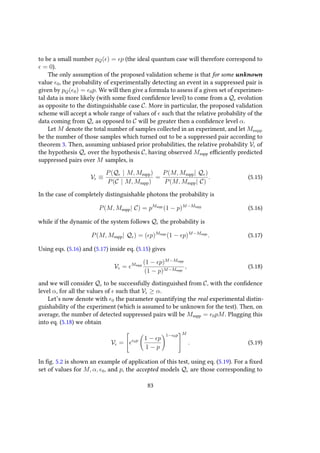
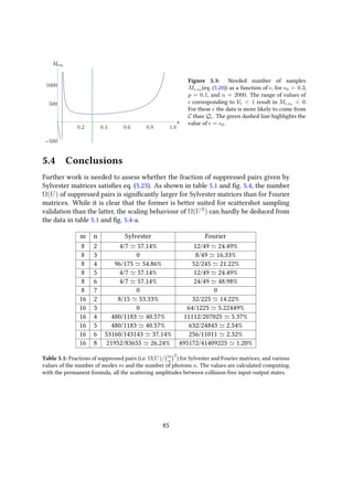
![8
16
32
64
128
m
5 10 15 20n
0
20
40
%
8
16
32
64
128
m
5 10 15 20n
0
10
20
30
40
a) b)
%
Figure 5.4: Estimated fraction of suppressed pairs with Fourier and Sylvester matrices. (a)
Fraction of suppressed pairs with Sylvester matrices, that is, Ω(US
)/ m
n
2
, plotted against n for various
values of m. The data is obtained randomly sampling N = 1000 input-output pairs, and computing the
permanent corresponding to each scattering amplitude. The percentage is known to be zero for number
of photons of the form n = 2p
− 1 [81], regardless of m. (b) Fraction of suppressed pairs with Fourier
matrices, that is, Ω(UF
)/ m
n
2
, plotted against n for various values of m. The fraction is in this case
significantly lower than for Sylvester matrices. For most values of n, no suppressed pair was found in
the sampled dataset.
In fig. 5.5 are again given the estimated fractions for Fourier and Sylvester matrices.
The error bars in fig. 5.5 represent the 99.7 % confidence interval, calculated through
Bayesian inference from the number of suppressed pairs found in the sampled datasets.
In particular, in fig. 5.5-a the fraction Ω(US
) depends weakly on m, as opposite to the
strong dependence of UF
on m shown in fig. 5.5-b.
Another relevant matter is the scaling with m and n of Ωeff(US
), that is, the number
of suppressed pairs satisfying the conditions of theorem 3. No efficiently evaluable
analytical expression is known for this number. Brute-force estimates are given in
fig. 5.6, where calculations similar to those in fig. 5.5 are shown, but this time for the
efficiently predictable suppressed pairs. In the presented cases of m = 16, 32, 64, 128,
Ωeff(US
) seems to decrease exponentially in n, for n < m/2.
In conclusion, while theorem 3 represents a significant improvement with respect
to theorem 1 and theorem 2, this fraction is probably still not large enough for an
efficient validation test with Sylvester matrices. However the data on the total fraction
of suppressed states presented in figs. 5.4 and 5.5 leaves open the possibility that, further
86](https://image.slidesharecdn.com/51b2159f-4e1f-48f3-91cc-51dca4e8cf7b-160331120712/85/thesis-86-320.jpg)
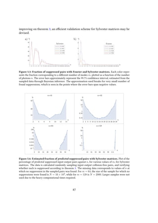

![Chapter 6
Experimental boson sampling
validation with integrated photonics
In this chapter we report the experimental implementation of the protocol devised
in [22, 24], and explained in section 4.2, and its use to validate quantum many-body
interference against alternative non-trivial hypotheses [25]. To this end, a scalable
approach for the implementation of the fast Fourier transform algorithm, using 3-D
photonic integrated interferometers, is developed. We observe the suppression law for
a large number of output states with 4- and 8-mode optical circuits. The experimental
results demonstrate genuine quantum interference between the injected photons. This
work provides a first experimental realization [25] of the validation protocol with
Fourier matrices [22] discussed in section 4.2 (during this work another experimental
realization of the same validation scheme was reported [17]). The reported experiments
were realized in the Quantum Optics laboratories at University of Rome La Sapienza.
In section 6.1 an overview of the work is given. In section 6.2 the femtosecond
laser-writing technique, employed to build the integrated photonic chips used in the
experiment, is described. In section 6.3 the quantum Fast Fourier Transform is described.
This is a linear optics generalization of the classical Fast Fourier Transform algorithm,
used in this work to implement efficiently the Fourier transformation on the integrated
interferometer. In section 6.4 we give a brief description of the photon generation
methods. In section 6.5 the results of the measurements are presented, focusing on the
observation of the Hong-Ou-Mandel dips and peaks, and the reconstruction of the chip
transformation. In section 6.6 we describe how the experimental results validate the
genuine many-boson quantum interference occuring in the interferometer, as opposite
to alternative models of evolution. Finally, in section 6.7, the results of the experiments
are discussed and the possible future prospects of this line of research.
89](https://image.slidesharecdn.com/51b2159f-4e1f-48f3-91cc-51dca4e8cf7b-160331120712/85/thesis-89-320.jpg)
![6.1 Overview of the experiment
We here report the experimental observation of the recently theoretically proposed [22]
suppression law for Fourier matrices, and its use to validate quantum many-body inter-
ference against alternative non-trivial hypotheses resulting in similar output probability
distributions.
The Fourier matrices have been implemented with an efficient and reliable approach
by exploiting the quantum version of the Fast Fourier Transform (qFFT), an algorithm
developed by Barak and Ben-Aryeh [26] to optimize the number of optical elements
required to build the Fourier transform over the optical modes.
Here we implement the qFFT on photonic integrated interferometers by exploiting
the 3-D capabilities of femtosecond laser writing [82, 83], which makes it possible to fab-
ricate waveguides arranged in three-dimensional structures with arbitrary layouts [13,
84, 85], by adopting an architecture scalable to a larger number of modes.
The observations have been carried out with two-photon Focks states injected into
4- and 8-mode qFFT interferometers. The peculiar behaviour of Fock states compared to
other kinds of states is investigated, showing in principle the validity of the certification
protocol for the identification of true granular n-particle interference, which is the
source of a rich landscape of quantum effects such as the computational complexity of
BosonSampling.
6.2 Femtosecond laser writing
Building large interferometers out of discrete, bulk optical elements tends to result in
mechanical instabilities which have prevented the demonstration of even a symmetric,
3-mode interferometer that preserves quantum coherence. A more promising approach
to obtain stable multi-mode interferometers involves the fabrication of this network of
linear optical elements by integrated optical waveguides in a glass chip [13, 84].
Waveguides are fabricated using the femtosecond laser micromachining technique
[83, 86], which exploits nonlinear absorption of focused femtosecond pulses to induce a
permanent and localized refractive index increase in transparent materials, as schemat-
ically shown in fig. 6.1. Arbitrary three-dimensional circuits can be directly written
by translating the sample along the desired path, keeping the velocity constant with
respect to the laser beam. This technique allows fast and cost-effective prototyping
of new devices, enabling the implementation of three-dimensional layouts that are
impossible to realize with conventional lithography.
90](https://image.slidesharecdn.com/51b2159f-4e1f-48f3-91cc-51dca4e8cf7b-160331120712/85/thesis-90-320.jpg)
![Figure 6.1: Laser-writing a waveguide on a
glass chip. The waveguide is fabricated focusing
femtosecond laser pulses to induce a permanent
and localized refractive index increase in transpar-
ent materials.
In the integrated optics approach the role of beam splitters is performed by direc-
tional couplers, devices which bring two waveguides close together to redistribute the
light propagating in them by evanescent field coupling (fig. 6.2-c). The phase shifters
are instead implemented by deforming the S-bent waveguides at the input of each
directional coupler in order to stretch the optical path (fig. 6.2-b). The integrated optics
analogue of a discrete components layout, depicted in fig. 6.3-a, is shown in fig. 6.3-b,
where one can appreciate the one-to-one correspondence between elements in the two
approaches.
TRANSMISSION CONTROL
PHASE-SHIFT CONTROL
0.00 0.05 0.10 0.15 0.20 0.25
0
1
2
3
4
5
d
Phaseshift[rad]
a
b
c
0 1 2 3 4 5 6
0.0
0.2
0.4
0.6
0.8
1.0
Angle [°]
Transmissivity
d [μm]
Transmission
Figure 6.2: Independent control of the phase shift and transmissivity at each directional cou-
pler. (a) The controlled deformation of the S-bent waveguide at the input of each directional coupler
and coupling geometry allows independent control over the phase shift and transmissivity. (b) The
deformation of the S-bent waveguide section is function of a deformation coefficient d. The graph
showed the undeformed S-bend together with a deformed one. (c) Control over the transmissivity of the
directional coupler is performed by modulating the coupling coefficient. This is achieved by changing
the waveguide spacing in the coupling region by rotating one arm of the directional coupler out of the
main circuit plane. A sample dependence of the the transmissivity as a function of the deformation angle
is provided. Credits: [10].
91](https://image.slidesharecdn.com/51b2159f-4e1f-48f3-91cc-51dca4e8cf7b-160331120712/85/thesis-91-320.jpg)
![t1 t2 t3 t4
t5 t6 t7
t8 t9
t10
IN
1
2
3
4
5
OUT
1
2
3
4
5
t1
t5 t6 t7
t2 t3 t4
t8 t9
t10
IN
1
2
3
4
5 5
4
3
2
1
OUT
a
b
tiαi
βi
tiαi
βi
Figure 6.3: Layout of multimode interferometers. (a) Realization of an arbitrary 5×5 mode trans-
formation via a network of beam splitters with different transmissivities ti. The blue and red boxes stand
for different phase shifters. (b) Implementation of the same scheme adopting integrated photonics. αi
and βi are parameters characterizing the phase shifts acquired by the photons passing through S-bend
waveguide segments. Credits: [10].
6.3 Realization of the quantum Fast Fourier Trans-
form
We here introduce an experimental implementation of the Fourier transformation with
the qFFT approach.
The general method to realize an arbitrary unitary transformation using linear
optics was introduced by Reck et al. [79], who provided a decomposition of an m×m
unitary as a sequence of m(m − 1)/2 beam splitters and phase shifters. However, in
the special case of Fourier matrices, a more efficient method has been proposed [26,
87], which takes advantage of their symmetries to significantly reduce the number of
linear optical elements required.
Based on the classical algorithm of Cooley and Tukey [27], who first introduced
the Fast Fourier Transform algorithm as a more efficient way to compute the discrete
92](https://image.slidesharecdn.com/51b2159f-4e1f-48f3-91cc-51dca4e8cf7b-160331120712/85/thesis-92-320.jpg)
![Fourier transform, Barak and Ben-Aryeh [26] developed a quantum analogue in the
linear optics domain, leading to the concept of qFFT. This approach, valid for 2p
-
dimensional Fourier matrices, requires only (m/2) log2 m beam splitters and phase
shifters, to be compared with the O(m2
) elements needed for the more general Reck
decomposition, thus enhancing the compactness and scalability of the platform for a
more reliable experimental realization.
The sequential structure arising from the decomposition of the m-dimensional
Fourier matrix using the Barak and Ben-Aryeh algorithm is reproduced by the con-
secutive layers shown in fig. 6.4. The complex arrangement of pairwise interactions
necessary for the qFFT method cannot be easily implemented using a planar architecture.
However, femtosecond laser writing technique allows to overcome this issue exploiting
the third dimension, arranging the waveguides along the bidimensional sections of the
integrated chip.
phase phasedirectional coupler directional coupler
4
3
2
1
4
3
2
1
31
6
42758
L1
L2
L1
L2
L3
P1
P2
P1
3
1
4
2
7
5
8
6
a b
L1 L2
42
31
P1 L1 L2P1 L3P2
⇡/23:
7:
8: 6:
8:
4:
⇡/2
⇡/2
⇡/2
⇡/4
3⇡/442
31
73
51
84
62
73
51
84
62
73
51
84
62
Figure 6.4: Schematic of the structure of the integrated devices. Internal structure of the 4-mode
(a) and 8-mode (b) integrated interferometers implementing the qFFT over the optical modes. The
mode arrangement has been chosen in a way to minimize bending losses. The insets shows the actual
disposition of the waveguides in the cross-section of the devices. The modes coupled together in each
step (Li) of the interferometer are joined by segments. The implemented phase shifts in each step (Pi)
are also indicated. Credits: [25].
The strategy can be outlined as follows: the 2p
modes are ideally placed on the
vertices of a p-dimensional hypercube, and in each step of the algorithm the vertices
connected by parallel edges having one specific direction are made to interact by a
2-mode Hadamard transformation, with proper phase terms. An optical interferometer
implementing this procedure is thus composed of log2 m = p sections, each employing
m/2 balanced beam splitters and phase shifters.
The waveguide interferometers were fabricated realizing the Fourier matrix for m =
4 and m = 8 modes in borosilicate glass chips using femtosecond laser micromachining
[83, 84]. A schematic representation of these two interferometers is given in fig. 6.4.
According to the scheme outlined above and by exploiting the three-dimensional
93](https://image.slidesharecdn.com/51b2159f-4e1f-48f3-91cc-51dca4e8cf7b-160331120712/85/thesis-93-320.jpg)
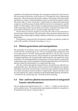
![a b
IF
HWP
PBS
PC
PDC output FA
input FA
chip
PBS
HWP
IF
PC
DL
DL
SMF
SMF
input FA
Figure 6.5: Experimental apparatus for input state preparation. (a) The photon source (IF: inter-
ferential filter, HWP: half-wave plate, PBS: polarizing beam splitter, PC: polarization compensator, PDC:
parametric downconversion, DL: delay lines with motorized stages, SMF: single-mode fiber). (b) Photon
injection (extraction) before (after) the evolution through the interferometer (FA: fiber array). Credits:
[25].
To test the validity of the suppression law, we measured the number of coincidences
at each forbidden output combination injecting cyclic inputs with two indistinguishable
photons. The degree of violation D of the suppression law could simply be evaluated
with a counting experiment. Alternatively, the same quantity D can be expressed as a
function of single-photon input-output probabilities and of the HOM visibilities, defined
as
Vi,j =
ND
i,j − NQ
i,j
ND
i,j
, (6.1)
where ND
i,j is the number of detected coincidences for distinguishable photons, NQ
i,j that
for indistinguishable photons, and the subscripts (i, j) are the indices of the two output
modes, for a given input state. The degree of violation can therefore be expressed as:
D =
Nforbidden
Nevents
= Pforbidden =
(i,j)forbidden
PQ
i,j =
(i,j)forbidden
PD
i,j(1 − Vi,j), (6.2)
where PQ
i,j (PD
i,j) are the probabilities of having photons in the outputs i, j in the
case of indistinguishable (distinguishable) particles. Here PD
i,j can be obtained from
single-particle probabilities. The visibilities are measured by recording the number of
coincidences for each output combination as a function of the temporal delay between
the two injected photons.
For the 4-mode device, we measured the full set of 4
2
= 36 collision-free input-
output combinations, that is, those combinations corresponding to the two photons
exiting from two different ports. These contributions have been measured by recording
95](https://image.slidesharecdn.com/51b2159f-4e1f-48f3-91cc-51dca4e8cf7b-160331120712/85/thesis-95-320.jpg)
![the number of coincidences for each combination of two outputs as a function of the
temporal delay between the two input photons. Due to the suppression law given in
theorem 1, we expect to observe four suppressed outcomes (over six possible output
combinations) for the two cyclic input states (1,3) and (2,4). Since distinguishable
photons exhibit no interference, HOM dips in the coincidence patterns are expected for
the suppressed output states. Conversely, peaks are expected in the non-suppressed
output combinations. The experimental results are shown in fig. 6.6, where the expected
pattern of four suppressions and two enhancements is reported, with average visibilities
of ¯Vsupp = 0.899 ± 0.001 and ¯Venh = −0.951 ± 0.004 for suppression and enhancement
respectively.
For the cyclic inputs, we also measured the interference patterns for the output
contributions where the two photons exit from the same mode. These terms have been
measured by inserting an additional symmetric beam splitter on each output mode,
and by connecting each of its two outputs to a single-photon detector. These cases
correspond to a full-bunching scenario with n = 2, and a HOM peak with V = −1
visibility is expected independently from the input state and from the unitary operation
[71]. This feature has been observed for the tested inputs, where an average visibility
of ¯Vbunch = −0.969 ± 0.024 has been obtained over all full bunching combinations.
The injection of non-cyclic input states has been employed for the complete recon-
struction of the chip action ˜UqFFT
4 , using a data set statistically independent from the
one adopted to observe the suppression law. The adopted reconstruction algorithm,
which exploits knowledge on the internal structure of the interfometers shown in
fig. 6.4, works in two steps. In a first step, the power-splitting ratios measured with
classical light are employed to extrapolate the transmissivities of the directional cou-
plers. In a second step, the two-photon visibilities for the non-cyclic inputs are used to
retrieve the values of the fabrication phases. In both steps, the parameters are obtained
by minimizing a suitable χ2
function. The results are shown in fig. 6.7. The fidelity
between the reconstructed unitary ˜UqFFT
4 and the theoretical Fourier transform UF
4 is
F = 0.9822 ± 0.0001, thus confirming the high quality of the fabrication process. The
error in the estimation of the fidelity is obtained through a Monte Carlo simulation,
properly accounting for the degree of distinguishability of the photons with a rescaling
factor in the visibilities.
96](https://image.slidesharecdn.com/51b2159f-4e1f-48f3-91cc-51dca4e8cf7b-160331120712/85/thesis-96-320.jpg)
![- 0.642(8)
2500
0.890(2)
2900
0.682(3)
2490
0.525(3)
2860
0.882(2)
2290
- 0.662(7)
2600
0.871(2)
2860
- 0.958(8)
2870
0.871(2)
2920
0.878(1)
3090
- 0.961(9)
2640
0.877(1)
3620
0.603(4)
1640
0.898(1)
4320
- 0.692(11)
1330
- 0.518(9)
1570
0.897(1)
2940
0.619(4)
1630
0.622(3)
3460
0.869(2)
3090
- 0.709(7)
3120
- 0.547(7)
2970
0.898(1)
3160
0.596(3)
2270
0.916(1)
3940
- 0.953(7)
3410
0.917(1)
3670
0.911(1)
3310
- 0.931(8)
2660
0.916(2)
2450
- 0.606(8)
2150
0.898(1)
4380
0.660(3)
3210
0.536(3)
3590
0.869(2)
3230
- 0.628(7)
2990
in (1,2)
in (1,3)
in (1,4)
in (2,3)
in (2,4)
in (3,4)
out (1,2) out (1,3) out (1,4) out (2,3) out (2,4) out (3,4)
Figure 6.6: Suppression law in a 4-mode Fourier integrated chip. Complete set of 36 measured
coincidence patterns (raw experimental data) for all input-output combinations in the 4-mode chip. For
each input-output combination, the measured coincidence pattern as a function of the time delay is
shown (points: experimental data, lines: best-fit curves). Cyclic inputs, highlighted in the picture, exhibit
enhancement (green) and suppression (red) on cyclic and non-cyclic outputs, respectively. For all points,
error bars are due to Poissonian statistics of the events. For each visibility, the error is obtained through a
Monte Carlo simulation by averaging over 3000 simulated data sets. In each plot the zero level coincides
with the baseline, while a dashed line represents the number of coincidence events in the distinguishable
limit. Credits: [25].
97](https://image.slidesharecdn.com/51b2159f-4e1f-48f3-91cc-51dca4e8cf7b-160331120712/85/thesis-97-320.jpg)
![VrecVqF F T VF
1 2 3 4
1
2
3
4
1 2 3 4
1
2
3
4
OUT
IN
0.4
0.45
4- 1/2
0.55
0.6
a)
b)
Figure 6.7: Suppression law in a 8-mode qFFT integrated chip. (a) HOM visibilities for all 36 input-
output configurations. From left to right: experimental measured visibilities (VqFFT, obtained from
raw experimental data), visibilities calculated from the reconstructed unitary (Vrec), and visibilities
calculated from the theoretical unitary (VF). (b) Representation of the reconstructed experimental
transformation ˜UqFFT
4 , and comparison with UF
4. Colored disks represent the moduli of the reconstructed
matrix elements (all equal to 4−1/2
for UF
4). Arrows represent the phases of the unitary matrix elements
(green: reconstructed unitary, blue: Fourier matrix). Credits: [25].
98](https://image.slidesharecdn.com/51b2159f-4e1f-48f3-91cc-51dca4e8cf7b-160331120712/85/thesis-98-320.jpg)
![For the 8-mode chip we recorded all the 8
2
= 28 two-photon coincidence patterns,
as a function of the relative delay between the input photons, for each of the 4 collision-
free cyclic inputs and for one non-cyclic input. The results are shown in fig. 6.8.
The reconstruction of the actual unitary transformation ˜UqFFT
8 implemented has been
performed with the same algorithm of the 4-modes, by using the power-splitting ratios
measured with classical light and the two-photon visibilities for one non-cyclic input.
The latter has been chosen in a way to maximize the sensitivity of the measurements
with respect to the five fabrication phases. The results are show in fig. 6.9. The fidelity
between the reconstructed unitary ˜UqFFT
8 and the ideal 8-mode Fourier transform UF
8 is
F = 0.9527 ± 0.0006.
0.800(6)
480
0.977(23)
480
0.844(6)
400
1.019(27)
350
0.772(9)
240
0.971(26)
360
0.850(6)
290
0.813(4)
980
0.856(20)
490
0.755(7)
440
0.895(24)
340
0.755(8)
270
0.838(19)
520
0.850(4)
690
0.890(25)
310
0.800(6)
480
0.960(24)
370
0.822(5)
590
0.790(7)
360
0.980(28)
260
0.824(5)
520
0.959(25)
300
0.796(7)
300
0.938(27)
260
0.765(9)
280
0.795(9)
250
0.875(27)
280
0.847(7)
380
out 1
out 2
out 3
out 4
out 5
out 6
out 7
out 2 out 3 out 4 out 5 out 6 out 7 out 8
Figure 6.8: Suppression law in a 8-mode qFFT integrated chip. Set of 28 measured coincidence
patterns (raw experimental data), corresponding to all collision-free output combinations for the input
(2,6) of the 8-mode interferometer. For each output combination, the measured coincidence pattern
as a function of the time delay is shown (points: experimental data, lines: best-fit curves). Red or
green backgrounds correspond to dips and peaks, respectively. For all points, error bars are due to
the Poissonian statistics of the events. For each visibility, the error is obtained through a Monte Carlo
simulation by averaging over 3000 simulated data sets. In each plot the zero level coincides with the
baseline, while a dashed line represents the number of coincidence events in the distinguishable limit.
Credits: [25].
99](https://image.slidesharecdn.com/51b2159f-4e1f-48f3-91cc-51dca4e8cf7b-160331120712/85/thesis-99-320.jpg)
![Average visibilities
(1,5) (2,6) (3,7) (4,8)
(1,5) (2,6) (3,7) (4,8)
- 0.25
- 0.5
- 0.75
- 1
0.25
0.5
0.75
1
1 2 3 4 5 6 7 8
1
2
3
4
5
6
7
8
1 2 3 4 5 6 7 8
1
2
3
4
5
6
7
8
OUT
IN
0.3
0.33
8- 1/2
0.38
0.4a) b)
Figure 6.9: Suppression law in a 8-mode qFFT integrated chip. (a) Average visibilities of dips
(red bars) and peaks (green bars) observed for the four collision-free cyclic inputs ((1,5),(2,6),(3,7),(4,8)).
Darker regions correspond to error bars of ±1 standard deviation. (b) Representation of the reconstructed
experimental transformation ˜UqFFT
8 , and comparison with UF
8. Colored disks represent the moduli of the
reconstructed matrix elements (all equal to 8−1/2
for UF
8). Arrows represent the phases of the unitary
matrix elements (green: reconstructed unitary, blue: Fourier matrix). Credits: [25].
6.6 Observation of the suppression law
The suppression of events which do not satisfy theorem 1 is fulfilled only when two
perfectly indistinguishable photons are injected in a cyclic input of a perfect Fourier
interferometer. In such a case, we would have the suppression of all output states such
that the sum of the elements of the corresponding MAL is odd. For the 4-mode (8-mode)
device, this corresponds to 4 (16) suppressed and 2 (12) non-suppressed collision-free
outputs (each one given by two possible arrangements of the two distinguishable
photons), plus 4 (8) terms with two photons in the same output, each one corresponding
to a single possible two-photon path.
The expected violation for distinguishable particles can be obtained from classical
considerations. Let us consider the case with n = 2. The two distinguishable photons
evolve independently from each other, and the output distribution is obtained by
classically mixing single-particle probabilities. All collision-free terms are equally likely
to occur with probability q = 2/m2
, while full-bunching events occur with probability
q = q/2 = 1/m2
. The degree of violation DD can then be obtained by multiplying the
probability q by the number of forbidden output combinations. As a result, we expect a
violation degree of DD = 0.5 for distinguishable two-photon states. The evaluation of
the expected value for a mean field state, which is due to single particle bosonic statistic
effects, require different calculations [22]. It can be shown that for n = 2 the degree of
violation is DMF = 0.25.
For each of the cyclic inputs, we have evaluated here the violation degree Dobs
100](https://image.slidesharecdn.com/51b2159f-4e1f-48f3-91cc-51dca4e8cf7b-160331120712/85/thesis-100-320.jpg)
![Figure 6.10: Observed violations Dobs as a function of the path difference |∆x| = c|∆τ| between the
two photons, for the 4-mode interferometer. Blue shaded regions in the plots correspond to the cases
where the hypothesis of distinguishable particles can be ruled out, and true two-particle interference is
present. Blue points: input (1,3). Red points: input (2,4). Blue solid line: theoretical prediction for input
(1,3). Red solid line: theoretical prediction for input (2,4). Black dashed line: theoretical prediction for a
Fourier matrix. (b) Data for the 8-mode interferometer. Blue points: input (1,5). Red points: input (2,6).
Green points: input (3,7). Magenta points: input (4,8). Colored solid lines: corresponding theoretical
predictions for different inputs. Black dashed line: theoretical prediction for a Fourier matrix. Table:
violations Dobs(0) at ∆x = 0 and discrepancies (in sigmas) with the expected values for distinguishable
particles (DD) and Mean Field Sampler (DMF), for the cyclic inputs of the two interferometer. Dobs(0)
are calculated following eq. (6.2), while expected values for the other two cases are DD = 0.5 and
DMF = 0.25. Error bars in all experimental quantities are due to the Poissonian statistics of measured
events. All theoretical predictions in solid lines are calculated from the reconstructed unitaries, obtained
from different sets of experimental data to ensure statistical independence. Credits: [25].
102](https://image.slidesharecdn.com/51b2159f-4e1f-48f3-91cc-51dca4e8cf7b-160331120712/85/thesis-102-320.jpg)
![Figure 6.11: Observed violations Dobs as a function of the path difference |∆x| = c|∆τ| between the
two photons, for the 8-mode interferometer. Blue shaded regions in the plots correspond to the cases
where the hypothesis of distinguishable particles can be ruled out, and true two-particle interference is
present. Blue points: input (1,5). Red points: input (2,6). Green points: input (3,7). Magenta points: input
(4,8). Colored solid lines: corresponding theoretical predictions for different inputs. Black dashed line:
theoretical prediction for a Fourier matrix. Table: violations Dobs(0) at ∆x = 0 and discrepancies (in
sigmas) with the expected values for distinguishable particles (DD) and Mean Field Sampler (DMF), for
the cyclic inputs of the two interferometer. Dobs(0) are calculated following eq. (6.2), while expected
values for the other two cases are DD = 0.5 and DMF = 0.25. Error bars in all experimental quantities
are due to the Poissonian statistics of measured events. All theoretical predictions in solid lines are
calculated from the reconstructed unitaries, obtained from different sets of experimental data to ensure
statistical independence. Credits: [25].
103](https://image.slidesharecdn.com/51b2159f-4e1f-48f3-91cc-51dca4e8cf7b-160331120712/85/thesis-103-320.jpg)
![6.7 Discussion
We have reported on the experimental observation of the suppression law on specific
output combinations of a Fourier transformation due to quantum interference between
photons. The observation of the suppression effect allowed us to rule out alternative
hypotheses to the Fock state. The use of a novel implementation architecture, enabled
by the 3-D capabilities of femtosecond laser micromachining, extends the scalability
of this technique to larger systems with lower experimental effort with respect to
other techniques. While the presented architecture is designed to implement a Fourier
matrix for a number of modes equal to m = 2p
, a generalization of the approach can be
obtained by adopting a building block different from the beam splitter. For devices of
odd dimension, for instance, such a tool can be provided by the tritter transformation
[13]. At the same time, the universality of a generalized HOM effect with an arbitrary
number of particles and modes is expected to make it a pivotal tool in the diagnostic and
certification of quantum photonic platforms. BosonSampling represents a key example,
since the scalability of the technique is expected to allow efficient certification of devices
outperforming their classical counterparts. An interesting open problem is whether the
computational hardness of BosonSampling is mantained if the randomness condition
is relaxed, and thus which is the minimal interferometric architecture required for an
evidence of post-classical computation.
Fourier matrices can find application in different contexts. For instance, multiport
beam splitters described by the Fourier matrix can be employed as building blocks for
multiarm interferometers, which can be adopted for quantum-enhanced single and
multiphase estimation protocols [88]. This would also allow the measurement of phase
gradients with precision lower than the shot-noise limit [89]. Other fields where Fourier
matrices are relevant include quantum communication scenarios [90], observation of
two-photon correlations as a function of geometric phase [91], fundamental quantum
information theory including mutually unbiased bases [92], as well as entanglement
generation [93].
104](https://image.slidesharecdn.com/51b2159f-4e1f-48f3-91cc-51dca4e8cf7b-160331120712/85/thesis-104-320.jpg)
![Conclusions
In this work we presented both theoretical and experimental advances in the context of
validating boson sampling experiments, both with the originally proposed approach
[8] and the recently proposed scattershot boson sampling scheme [19, 20].
From the theoretical point of view, the existing validation techniques have been
analysed in light of the recently proposed, and experimentally implemented, scattershot
boson sampling scheme [18, 19, 20]. We found that the existing methods to validate
genuine many-boson interference cannot be efficiently applied to scattershot boson
sampling experiments. Subsequently, we devised a new Zero-Transmission Law (ZTL)
for Sylvester matrices which has dramatically higher predictive capabilities with respect
to previously proposed ZTLs [23, 24]. We studied the fraction of suppressed input-output
pairs predicted by this ZTL, and its scaling with the number of photons n and the number
of modes m. We found that the number of predicted suppressed input-output pairs,
while significantly higher than that presented by previous ZTLs, still scales badly with n,
decreasing exponentially. However, it is less clear how the total number of suppressed
pairs in Sylvester matrices actually scales. Brute-force computations are not possible
beyond relatively small numbers of n, but the data gathered so far shows a rather
complex behaviour, which leaves open the possibility that this ratio decreases only
polynomially with n and m. Further work is needed in this direction to conclusively
assess whether an efficient validation scheme based on Sylvester matrices is possible,
but what is currently known leaves open this possibility.
From the experimental point of view, we reported on the first implementation of
a validation scheme [22] based on a ZTL for Fourier matrices [24]. This was realized
using integrated photonics technology, with 2 photons injected into 4- and 8-mode in-
terferometers realized on glass chips with femtosecond laser writing technique. A novel
methodology to efficiently implement a 2p
-dimensional Fourier matrix was employed,
exploiting the 3-D capabilities of femtosecond laser writing to implement the Barak and
Ben-Aryeh [26] quantum optics generalization of the Fast Fourier Transform algorithm
[27]. A thorough analysis of the Hong-Ou-Mandel dips and peaks corresponding to
the various possible configurations of 2-photon input-output pairs is reported, and
the transition from distinguishable to indistinguishable photons studied, showing an
excellent agreement with the predictions of quantum mechanics. An algorithm to effi-
105](https://image.slidesharecdn.com/51b2159f-4e1f-48f3-91cc-51dca4e8cf7b-160331120712/85/thesis-105-320.jpg)
![ciently reconstruct the unitary matrix implemented in the device is presented, showing
a good agreement with the ideal Fourier matrix. Finally, the efficient validation scheme
proposed in [22] is implemented, finding a perfect match with the expected pattern of
suppressions, and ruling out alternative models such as distinguishable particles and
Mean Field sampler [22].
106](https://image.slidesharecdn.com/51b2159f-4e1f-48f3-91cc-51dca4e8cf7b-160331120712/85/thesis-106-320.jpg)

![Bibliography
[1] Richard P Feynman. “Simulating physics with computers”. In: International jour-
nal of theoretical physics 21.6/7 (1982), pp. 467–488.
[2] John Preskill. Quantum computing and the entanglement frontier. 2012. arXiv:
1203.5813 [quant-ph].
[3] John Preskill. Supremacy Now? 2012. url: http://quantumfrontiers.
com/2012/07/22/supremacy-now/ (visited on 10/27/2015).
[4] John Preskill. Fault-tolerant quantum computation. 1998. arXiv: quant-ph/
9712048.
[5] Emanuel Knill, Raymond Laflamme, and Wojciech H Zurek. “Resilient quantum
computation”. In: Science 279.5349 (1998), pp. 342–345.
[6] Dorit Aharonov and Michael Ben-Or. “Fault-tolerant quantum computation with
constant error rate”. In: SIAM Journal on Computing 38.4 (2008), pp. 1207–1282.
arXiv: quant-ph/9906129.
[7] Emanuel Knill, Raymond Laflamme, and Gerald J Milburn. “A scheme for efficient
quantum computation with linear optics”. In: nature 409.6816 (2001), pp. 46–52.
[8] Scott Aaronson and Alex Arkhipov. “The computational complexity of linear
optics”. In: Proceedings of the forty-third annual ACM symposium on Theory of
computing. ACM. 2011, pp. 333–342. arXiv: 1011.3245 [quant-ph].
[9] Matthew A Broome et al. “Photonic boson sampling in a tunable circuit”. In:
Science 339.6121 (2013), pp. 794–798. arXiv: 1212.2234 [quant-ph].
[10] Andrea Crespi et al. “Integrated multimode interferometers with arbitrary designs
for photonic boson sampling”. In: Nature Photonics 7.7 (2013), pp. 545–549. arXiv:
1212.2783 [quant-ph].
[11] Max Tillmann et al. “Experimental boson sampling”. In: Nature Photonics 7.7
(2013), pp. 540–544. arXiv: 1212.2240 [quant-ph].
[12] Justin B Spring et al. “Boson sampling on a photonic chip”. In: Science 339.6121
(2013), pp. 798–801. arXiv: 1212.2622 [quant-ph].
109](https://image.slidesharecdn.com/51b2159f-4e1f-48f3-91cc-51dca4e8cf7b-160331120712/85/thesis-109-320.jpg)
![[13] Nicolò Spagnolo et al. “Three-photon bosonic coalescence in an integrated tritter”.
In: Nature communications 4 (2013), p. 1606. arXiv: 1210.6935 [quant-
ph].
[14] Nicolò Spagnolo et al. “Experimental validation of photonic boson sampling”. In:
Nature Photonics 8.8 (2014), pp. 615–620. arXiv: 1311.1622 [quant-ph].
[15] Jacques Carolan et al. “On the experimental verification of quantum complexity
in linear optics”. In: Nature Photonics 8.8 (2014), pp. 621–626. arXiv: 1311.2913
[quant-ph].
[16] Jacques Carolan et al. “Verifying quantum complexity in linear optical experi-
ments”. In: CLEO: QELS_Fundamental Science. Optical Society of America. 2014,
FM2A–7.
[17] Jacques Carolan et al. “Universal linear optics”. In: Science 349.6249 (2015), pp. 711–
716. doi: 10.1126/science.aab3642. arXiv: 1311.2913 [quant-
ph]. url: http://www.sciencemag.org/content/349/6249/
711.abstract.
[18] Marco Bentivegna et al. “Experimental scattershot boson sampling”. In: Science
Advances 1.3 (2015), e1400255. arXiv: 1515.03708 [quant-ph].
[19] Scott Aaronson. Scattershot BosonSampling: A new approach to scalable Boson-
Sampling experiments. 2013. url: http://www.scottaaronson.com/
blog/?p=1579 (visited on 12/22/2015).
[20] AP Lund et al. “Boson sampling from a Gaussian state”. In: Physical review letters
113.10 (2014), p. 100502.
[21] Scott Aaronson and Alex Arkhipov. “Bosonsampling is far from uniform”. In:
Quantum Information & Computation 14.15-16 (2014), pp. 1383–1423.
[22] Malte C Tichy et al. “Stringent and efficient assessment of boson-sampling de-
vices”. In: Physical review letters 113.2 (2014), p. 020502. arXiv: 1312.3080
[quant-ph].
[23] Andrea Crespi. “Suppression laws for multiparticle interference in Sylvester
interferometers”. In: Physical Review A 91.1 (2015), p. 013811. arXiv: 1502.
06372 [quant-ph].
[24] Malte Christopher Tichy et al. “Zero-transmission law for multiport beam split-
ters”. In: Physical review letters 104.22 (2010), p. 220405. arXiv: 1002.5038
[quant-ph].
[25] Andrea Crespi et al. “Quantum suppression law in a 3-D photonic chip implement-
ing the Fast Fourier Transform”. In: (2015). arXiv: 1508.00782 [quant-
ph].
110](https://image.slidesharecdn.com/51b2159f-4e1f-48f3-91cc-51dca4e8cf7b-160331120712/85/thesis-110-320.jpg)
![[26] Ronen Barak and Yacob Ben-Aryeh. “Quantum fast Fourier transform and quan-
tum computation by linear optics”. In: JOSA B 24.2 (2007), pp. 231–240.
[27] James W Cooley and John W Tukey. “An algorithm for the machine calculation of
complex Fourier series”. In: Mathematics of computation 19.90 (1965), pp. 297–301.
[28] Michael A Nielsen and Isaac L Chuang. Quantum computation and quantum
information. Cambridge university press, 2010.
[29] Robert Solovay and Volker Strassen. “A fast Monte-Carlo test for primality”. In:
SIAM journal on Computing 6.1 (1977), pp. 84–85.
[30] Peter W Shor. “Polynomial-time algorithms for prime factorization and discrete
logarithms on a quantum computer”. In: SIAM journal on computing 26.5 (1997),
pp. 1484–1509. arXiv: quant-ph/9508027.
[31] Lane A Hemaspaandra. “Sigact news complexity theory column 36”. In: ACM
SIGACT News 33.2 (2002), pp. 34–47.
[32] Scott Aaronson. The Scientific Case for P != NP. 2014. url: http://www.
scottaaronson.com/blog/?p=1720 (visited on 11/30/2015).
[33] Scott Aaronson. “Guest column: NP-complete problems and physical reality”. In:
ACM Sigact News 36.1 (2005), pp. 30–52.
[34] Leslie G Valiant. “The complexity of computing the permanent”. In: Theoretical
computer science 8.2 (1979), pp. 189–201.
[35] Charles H Bennett and David P DiVincenzo. “Quantum information and compu-
tation”. In: Nature 404.6775 (2000), pp. 247–255.
[36] Ryszard Horodecki et al. “Quantum entanglement”. In: Reviews of Modern Physics
81.2 (2009), p. 865.
[37] Otfried Gühne and Géza Tóth. “Entanglement detection”. In: Physics Reports 474.1
(2009), pp. 1–75.
[38] Seth Lloyd. “Universal quantum simulators”. In: SCIENCE-NEW YORK THEN
WASHINGTON- (1996), pp. 1073–1077.
[39] Bryan T Gard et al. “An introduction to boson-sampling”. In: arXiv preprint
arXiv:1406.6767 (2014).
[40] Pieter Kok et al. “Linear optical quantum computing with photonic qubits”. In:
Reviews of Modern Physics 79.1 (2007), p. 135. arXiv: quant-ph/0512071.
[41] Henryk Minc. Permanents. Vol. 6. Cambridge University Press, 1984.
[42] MD Eisaman et al. “Invited review article: Single-photon sources and detectors”.
In: Review of Scientific Instruments 82.7 (2011), p. 071101.
111](https://image.slidesharecdn.com/51b2159f-4e1f-48f3-91cc-51dca4e8cf7b-160331120712/85/thesis-111-320.jpg)
![[43] Brahim Lounis and Michel Orrit. “Single-photon sources”. In: Reports on Progress
in Physics 68.5 (2005), p. 1129.
[44] Christopher Gerry and Peter Knight. Introductory quantum optics. Cambridge
university press, 2005.
[45] Romain Alléaume et al. “Experimental open-air quantum key distribution with a
single-photon source”. In: New Journal of physics 6.1 (2004), p. 92.
[46] T Gaebel et al. “Stable single-photon source in the near infrared”. In: New Journal
of Physics 6.1 (2004), p. 98.
[47] E Wu et al. “Room temperature triggered single-photon source in the near in-
frared”. In: New Journal of Physics 9.12 (2007), p. 434.
[48] Satoshi Kako et al. “A gallium nitride single-photon source operating at 200 K”.
In: Nature materials 5.11 (2006), pp. 887–892.
[49] Andrew J Shields. “Semiconductor quantum light sources”. In: Nature photonics
1.4 (2007), pp. 215–223.
[50] Stefan Strauf et al. “High-frequency single-photon source with polarization
control”. In: Nature photonics 1.12 (2007), pp. 704–708.
[51] Markus Hennrich et al. “Photon statistics of a non-stationary periodically driven
single-photon source”. In: New Journal of Physics 6.1 (2004), p. 86.
[52] Christian Maurer et al. “A single-photon source based on a single Ca ion”. In:
New journal of physics 6 (2004), pp. 94–94.
[53] Mathias Steiner et al. “Highly efficient, tunable single photon source based on
single molecules”. In: Applied physics letters 18 (2007).
[54] Shuai Chen et al. “Deterministic and storable single-photon source based on a
quantum memory”. In: Physical review letters 97.17 (2006), p. 173004.
[55] S Cova et al. “Evolution and prospects for single-photon avalanche diodes and
quenching circuits”. In: Journal of Modern Optics 51.9-10 (2004), pp. 1267–1288.
[56] S Komiyama et al. “A single-photon detector in the far-infrared range”. In: Nature
403.6768 (2000), pp. 405–407.
[57] Kristine M Rosfjord et al. “Nanowire single-photon detector with an integrated
optical cavity and anti-reflection coating”. In: Optics Express 14.2 (2006), pp. 527–
534.
[58] Marius A Albota and Franco NC Wong. “Efficient single-photon counting at
1.55 µm by means of frequency upconversion”. In: Optics letters 29.13 (2004),
pp. 1449–1451.
[59] Hiroki Takesue et al. “1.5-µm single photon counting using polarization-independent
up-conversion detector”. In: Optics express 14.26 (2006), pp. 13067–13072.
112](https://image.slidesharecdn.com/51b2159f-4e1f-48f3-91cc-51dca4e8cf7b-160331120712/85/thesis-112-320.jpg)
![[60] Robert Thomas Thew et al. “Low jitter up-conversion detectors for telecom
wavelength GHz QKD”. In: New Journal of Physics 8.3 (2006), p. 32.
[61] Kendall B Davis et al. “Bose-Einstein condensation in a gas of sodium atoms”. In:
Physical review letters 75.22 (1995), p. 3969.
[62] Mike H Anderson et al. “Observation of Bose-Einstein condensation in a dilute
atomic vapor”. In: science 269.5221 (1995), pp. 198–201.
[63] Jan Klaers et al. “Bose-Einstein condensation of photons in an optical microcavity”.
In: Nature 468.7323 (2010), pp. 545–548.
[64] CK Hong, ZY Ou, and Leonard Mandel. “Measurement of subpicosecond time
intervals between two photons by interference”. In: Physical Review Letters 59.18
(1987), p. 2044.
[65] Malte C Tichy. “Interference of identical particles from entanglement to boson-
sampling”. In: Journal of Physics B: Atomic, Molecular and Optical Physics 47.10
(2014), p. 103001. arXiv: 1312.4266 [quant-ph].
[66] Malte Christopher Tichy. “Entanglement and interference of identical particles”.
PhD thesis. Universitätsbibliothek Freiburg, 2011.
[67] VS Shchesnovich. “Asymptotic evaluation of bosonic probability amplitudes in
linear unitary networks in the case of large number of bosons”. In: International
Journal of Quantum Information 11.05 (2013), p. 1350045.
[68] David G Glynn. “The permanent of a square matrix”. In: European Journal of
Combinatorics 31.7 (2010), pp. 1887–1891.
[69] Lidror Troyansky and Naftali Tishby. “Permanent uncertainty: On the quantum
evaluation of the determinant and the permanent of a matrix”. In: Proc. 4th
Workshop on Physics and Computation (PhysComp’96). 1996.
[70] Annalisa Marzuoli and Mario Rasetti. “Towards a quantum algorithm for the
permanent”. In: International Journal of Quantum Information 5.01n02 (2007),
pp. 223–228.
[71] Nicolò Spagnolo et al. “General rules for bosonic bunching in multimode inter-
ferometers”. In: Physical review letters 111.13 (2013), p. 130503.
[72] VS Shchesnovich. “Sufficient condition for the mode mismatch of single photons
for scalability of the boson-sampling computer”. In: Physical Review A 89.2 (2014),
p. 022333.
[73] Peter P Rohde et al. “Will boson-sampling ever disprove the Extended Church-
Turing thesis?” In: arXiv preprint arXiv:1401.2199 (2014).
[74] Peter P Rohde and Timothy C Ralph. “Error tolerance of the boson-sampling
model for linear optics quantum computing”. In: Physical Review A 85.2 (2012),
p. 022332.
113](https://image.slidesharecdn.com/51b2159f-4e1f-48f3-91cc-51dca4e8cf7b-160331120712/85/thesis-113-320.jpg)
![[75] Anthony A Leverrier and Raul Garcia-Patron Sanchez. “Analysis of circuit im-
perfections in BosonSampling”. In: Quantum information & computation 15.5-6
(2015), pp. 489–512.
[76] Alberto Peruzzo et al. “Quantum walks of correlated photons”. In: Science 329.5998
(2010), pp. 1500–1503. arXiv: 1006.4764 [quant-ph].
[77] C Gogolin et al. “Boson-sampling in the light of sample complexity”. In: arXiv
(2013). arXiv: 1306.3995 [quant-ph].
[78] Anthony Laing and Jeremy L O’Brien. “Super-stable tomography of any linear
optical device”. In: arXiv preprint arXiv:1208.2868 (2012).
[79] Michael Reck et al. “Experimental realization of any discrete unitary operator”.
In: Physical Review Letters 73.1 (1994), p. 58.
[80] Alex Arkhipov and Greg Kuperberg. “The bosonic birthday paradox”. In: Geome-
try & Topology Monographs 18 (2012), pp. 1–7.
[81] Rodica Simion and Frank W Schmidt. “On (+ 1,- 1)-matrices with vanishing
permanent”. In: Discrete Mathematics 46.1 (1983), pp. 107–108.
[82] Roberto Osellame et al. “Femtosecond writing of active optical waveguides with
astigmatically shaped beams”. In: JOSA B 20.7 (2003), pp. 1559–1567.
[83] Rafael R Gattass and Eric Mazur. “Femtosecond laser micromachining in trans-
parent materials”. In: Nature photonics 2.4 (2008), pp. 219–225.
[84] Thomas Meany et al. “Non-classical interference in integrated 3D multiports”.
In: Optics express 20.24 (2012), pp. 26895–26905.
[85] Konstantinos Poulios et al. “Quantum walks of correlated photon pairs in two-
dimensional waveguide arrays”. In: Physical review letters 112.14 (2014), p. 143604.
[86] G Della Valle, R Osellame, and P Laporta. “Micromachining of photonic devices
by femtosecond laser pulses”. In: Journal of Optics A: Pure and Applied Optics 11.1
(2009), p. 013001.
[87] P Törmä, I Jex, and S Stenholm. “Beam splitter realizations of totally symmetric
mode couplers”. In: journal of modern optics 43.2 (1996), pp. 245–251.
[88] Nicolò Spagnolo et al. “Quantum interferometry with three-dimensional geome-
try”. In: Scientific reports 2 (2012).
[89] Keith R Motes et al. “Linear Optical Quantum Metrology with Single Photons:
Exploiting Spontaneously Generated Entanglement to Beat the Shot-Noise Limit”.
In: Physical review letters 114.17 (2015), p. 170802.
[90] Saikat Guha. “Structured optical receivers to attain superadditive capacity and
the Holevo limit”. In: Physical review letters 106.24 (2011), p. 240502.
114](https://image.slidesharecdn.com/51b2159f-4e1f-48f3-91cc-51dca4e8cf7b-160331120712/85/thesis-114-320.jpg)
![[91] Anthony Laing et al. “Observation of quantum interference as a function of
Berry’s phase in a complex Hadamard optical network”. In: Physical review letters
108.26 (2012), p. 260505.
[92] Ingemar Bengtsson et al. “Mutually unbiased bases and Hadamard matrices of
order six”. In: Journal of mathematical physics 48.5 (2007), p. 052106.
[93] Yuan Liang Lim and Almut Beige. “Multiphoton entanglement through a Bell-
multiport beam splitter”. In: Physical Review A 71.6 (2005), p. 062311.
115](https://image.slidesharecdn.com/51b2159f-4e1f-48f3-91cc-51dca4e8cf7b-160331120712/85/thesis-115-320.jpg)