This document summarizes a master's thesis on optimizing quantum states for phase sensitivity in quantum interference measurements. The thesis investigates the fundamental sensitivity limits of two-mode interferometry in the presence of photon loss. It develops a computer algorithm to find the optimal quantum states for N=2 and 3 photons and compares their performance to the standard quantum limit. While focusing on practical implementation possibilities, it provides a comprehensive discussion of statistical methods and their potential for realizing optimized measurements.

![Introduction
Interferometry is a technique, which possesses a truly supreme potential when high precison of measurements
is a required. After the invention of laser by Shawlow and Townes and its demonstration by Maiman
in 1960, interferometry has found a great number of applications, where metrology, astronomy, surface
scanning, remote sensing, telecommunications are just few examples (Ref. [13]). However, as the demand
for precision, especially in scientific areas such as gravitational wave detection and quantum information,
constantly increases, the questions of the the sensitivity limits become more and more important.
It turns out that, even in the absence of any external sources of noise, classical light is, in its nature,
a stochastic process, which imposes bounds to precision of phase measurements. Although, these bounds
cannot be overcome by any classical means, quantum optics promises the sensitivity beyond that limit. This
promise, also known as phase super-sensitivity, became a research area, whose exploration started around
fifteen years ago. Various methods have been proposed by different groups (Refs. [5, 7, 11, 21, 22, 23]) in order
to reach the quantum improvement. However, no super-sensitivity has been experimentally demonstrated
with using quantum states of more than N = 4 photons until now (Ref. [6, 7]). As the phase sensitivity is
closely related to specific quantum states of light used for the measurement, the ‘race’ to find the optimal
states has begun. In 2007, P. Meystre and H. Uys (Ref. [2]) were the first who conducted a systematic
search for such states, although, at that stage no losses were accounted in the mathematical model. In 2009,
Demkowicz-Dobrza´nski, et al. (Ref. [3]) found the optimal states under the presence of loss. However, the
specific assumptions they made concerning both the accessable quantum information and detection strategy,
gave their research purely theoretical character.
In this thesis work, the phase sensitivity limit is investigated with a strong empahsis put on practically
implementable methods and strict resource limits (photons) used in the measurement. The optimal states
are being found, by extending the methods developed by Ref. [2] to account for the presence of photon
loss. Contrary to Ref. [3], we have assumed non-optimised detection scheme. Still, certain practical issues,
such as the experimental cost of preparing the quantum states and non-ideal detection network, although
mentioned, are not particularly focused on.
The thesis is organised as follows: In Chapter I, a very brief introduction (or rather revision) of the some
useful quantum optical concepts is made. The mathematical description of qunatisized light and relevant
optical components is given and the interferometric setup is presented using the quantum ‘language’. Chapter
II defines the phase sensitivity and introduces statistical methods that are indespensable to analyse the
measurements’ outcomes. Two important statistical theories are presented and compared in the context of
the detection strategy that helps us to evaluate the criterion for optimisation. Having both, the system and
the statistical tools defined, the optimisation procedure and the results are presented in Chapter III. Finally,
a concluding discussion is made.
Last, but not least, it should be noted at this stage that with the strongest and honest aspiration to
discover something new, I was not the first person, who pursued this idea. Lee, et al. (Ref. [4]) published
independently, and unknown to me, almost identical the result in December 2009. Although I was not aware
of their publictaion until almost the very end days of my research, still the confrontation of my results shows
a perfect match between our data. See Section 3.4 for more details.
3](https://image.slidesharecdn.com/2d2c0242-172a-41b4-b64f-baad53159f08-160925145102/85/MSc_thesis_OlegZero-5-320.jpg)
![1.1.2 Phase Shifter
In Quantum Optics, the phase shift is fundamentally related to the time-evolution of the state (Ref. [1]).
What is more, the light mode itself is analogous to quantum harmonic oscillator. Therefore, the Hamiltonian
responsible for the phase shift is the harmonic oscillator Hamiltonian:
ˆH = ω ˆa†
ˆa +
1
2
= ω ˆn +
1
2
(1.4)
The unitary operator responsible for the phase shift transformation can be found by solving the time-
dependent Schr¨odinger equation using this Hamiltonian. In the Fock state basis, this operator reads:
ˆUϕ = e−i ˆHt/
= e−iωtˆn
= e−iϕˆn
(1.5)
Note that, the ω/2 is a common factor and hence it may be skipped without any consequences. To ilustrate,
let us take the eq. (1.1) and use this operator:
ˆUϕ|ψ =
∞
n=0
cne−iϕˆn
|n =
∞
n=0
cne−iϕn
|n (1.6)
The Fock states are the eigenstates of the photon number operator ˆn, which is why we can write ˆn|n = n|n .
As we can see, different Fock components existing within the superposition acquire different phase shifts that
are directly proportional to the photon number.
1.1.3 Beam Splitter
In most general terms, a beam splitter is a four-port1
that combines two optical modes and transforms them
into another two modes. From the quantum point of view, this situation corresponds to having two coupled
harmonic oscillators , where the coupling is described by the following Hamiltonian (Ref. [1]):
ˆH = κ(ˆa†ˆb + ˆaˆb†
) (1.7)
The operators: ˆa, ˆa†
and ˆb, ˆb†
refer to the first and second beam splitter’s inputs respectively and the κ is
related to the coupling modes’ interaction time giving us the coupling strength
Again, we would be interested in finding an explicit form of the unitary operator that is responsible for
the beam splitter’s tranformation:
ˆUBS = e−iκt(ˆa†ˆb + ˆaˆb†
)
(1.8)
However, since this operator would not operate in the its eigenbasis, and therefore, a way to handle this
problem is to define the following subsititution of creation operators:
ˆa† BS
−−→ ˆa†
cos κt + ˆb†
sin κt
ˆb† BS
−−→ ˆb†
cos κt − ˆa†
sin κt
(1.9)
This set of “equations” can be derived from the time-evolution of the annihilation operators in the Heisenberg
picture, using an equivalent Hamiltonian2
: ˆH = i κ(ˆa†ˆb − ˆaˆb†
).
Substituting:
√
ξ = cos κt and
√
1 − ξ = sin κt, when ξ ∈ [0, 1], we can also state (1.9) the more convinient
form:
ˆa† BS
−−→ ˆa†
√
ξ + ˆb†
√
1 − ξ
ˆb† BS
−−→ ˆb†
√
ξ − ˆa†
√
1 − ξ
(1.10)
Now, we can clearly refer ξ to the beam splitter’s transmittivity. If we set ξ → 0.5, we obtain the
transformation for the 50:50 beam splitter. Similarly, setting ξ → 0 turns our beam splitter into a perfect
mirror.
1Although, in this context, the beam splitters are used as two-ports
2This Hamiltonian represents exactly the same physical truth. What is more, its form also preserves the hermicity. Therefore,
the choice between (1.7) and this Hamiltonian is purely the matter of convinience.
5](https://image.slidesharecdn.com/2d2c0242-172a-41b4-b64f-baad53159f08-160925145102/85/MSc_thesis_OlegZero-7-320.jpg)
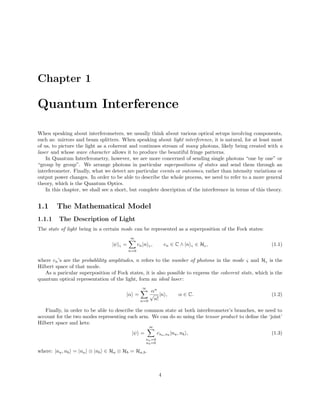
![1.2 The Interferometric Setup
The interferometric setup considered in this work is the Mach-Zehnder (MZ) interferometer. This setup is a
fairly simple, but also a powerful tool for performing phase measurements. As we know, in its purest form,
the MZ consists of two branches or arms: A and B, from which at one, the light is induced the relative
phase shift: ϕ and the other one serves as the referrence beam. Both arms are coupled through beam splitters
(BS) and the relative phase shift is induced by the phase shifter (PS). The PS may in fact refer to just any
material or region of space that changes the optical path difference between the two arms.
Figure 1.1: The schamtic of the Mach-Zehnder interferometer.
Traditionally, for the MZ interfometer3
, we can discriminate three specific regions. Region I is the
interferometer’s input stage, which is where the light enters the setup. The first beam splitter, then splits
the mode into two, after which we define the region II – the MZ’s internal part. Finally, the second beam
splitter recombines the modes, after which we define the interferometer’s output – the region III.
1.2.1 Lossless Case
When no loss is present, then our MZ is just what we can see on the Fig. 1.1. We assume an arbitrary pure
input state |ψin of the follwoing form:
|ψin =
∞
n1=0
n2=0
xn1n2
|n1, n2 (1.11)
When light propagates through the interferometer, the state (1.11) undergoes the following three transfor-
mations (Ref. [2]), in the consecutive order:
|ψout(ϕ) = ˆUBS2
ˆUϕ
ˆUBS1
|ψin (1.12)
Under these transformations, we obtain the output state |ψout(ϕ) , which is also a pure state but, whoose
output components’ amplitudes interfere with each other in various ways
|ψout(ϕ) =
∞
n1=0
n2=0
yn1n2 (ϕ)|n1, n2 (1.13)
This interference gives rise to phase-dependent probablility distributions for the outcomes, which are the pos-
sible numbers of photons, leaving the interferometer at each branch: (n1, n2). Analysing those distributions,
we learn about the phase.
Finally, it should also be mentioned that most often, the total number of particles N used in a single
measurement is known and fixed. In these cases: (n1, n2) ≡ (k, N − k) and the outcomes can be identified
by the single number k ∈ [0, N] ⊂ N.
3It is also true for other setup configurations, such as: the Michelson, Fabry-P´erot or Sagnac interferometer. Although the
geometry of those setups are arragned differently, one can still discriminate between the three parts and the whole analysis can
be carried out with the same methods. The choice of the MZ originates from the simplicity of its form.
6](https://image.slidesharecdn.com/2d2c0242-172a-41b4-b64f-baad53159f08-160925145102/85/MSc_thesis_OlegZero-8-320.jpg)
![1.2.2 Lossy Case
In realistic situations, the interferometer can never be absolutely lossless. In particular, photons can be lost
due to the interferometer’s imperfections, and due to possible loss existing in the sample. Whenever any of
these mechanisms is present, the possibility one or more photons, needs to be accounted in the mathematical
model.
Figure 1.2: The Mach-Zehnder interferometer with losses.
The Model of Loss
To account for the loss, our MZ is now equipped with two additional fictous beam splitters (Refs. [3, 8, 9, 10]):
BSη
1 and BSη
2 with variable transmission parameters: η1 and η2, as can be seen on the Fig. 1.2. The fictous
beam splitters mimic losses by sending photons to the loss modes (3) and (4), which can be understood as
an extention to interferometer’s Hilbert space. Again, we use the tensor product to define the joint space:
|n1, n2; 1, 2 ∈ H1,2 ⊗ H
(loss)
3,4 (1.14)
For any ket, the numbers: 1 and 2 denote how many photons are lost at the first or the second arm,
respectively. The creation operators to the loss modes are: ˆa†
η and ˆb†
η, and the transformation can be defined
in similar way to (1.10):
ˆa† BSη
1
−−−→ ˆa†√
η1 + ˆa†
η
√
1 − η1
ˆb† BSη
2
−−−→ ˆb†√
η2 + ˆb†
η
√
1 − η2
(1.15)
In any real situation, we do not have any means to trace the lost photons. Therefore, we must literally
trace-out the two additional modes, which leaves us with a mixed state that is described by the reduced
density matrix.
The “Families” of States
Let us have a closer look at what happens to the state in the inerferometer. After the 1st beam splitter, the
input state |ψin becomes the internal state, which undergoes the phase shift and the loss-transformation.
It can be expressed as follows:
|ψint(ϕ) =
n1,n2 1, 2
γ( 1, 2)
n1,n2
(ϕ) |n1, n2; 1, 2 , (1.16)
where n1 and n2 are limited by the total number of photons N, and 1, 2 are limited by n1, n2. The complete
density matrix of that state is:
ˆρint = |ψint(ϕ) ψint(ϕ)| =
=
n1,n2
n1,n2
1, 2
1, 2
γ( 1, 2)
n1,n2
γ
( 1, 2)
n1,n2
∗
|n1 − 1, n2 − 2; 1, 2 n1 − 1, n2 − 2; 1, 2| (1.17)
7](https://image.slidesharecdn.com/2d2c0242-172a-41b4-b64f-baad53159f08-160925145102/85/MSc_thesis_OlegZero-9-320.jpg)
![Chapter 2
Beyond Classical Meausurements
Now, after we have seen of how the Mach-Zehnder interferometer is treated by quantum optics, including
also the model of loss, we are ready to move on to the next stage. In this chapter, we are going to “forget”
for a moment about the detailed analysis of the MZ itself. Instead, we will concentrate more on what it
means to make a good measurement in terms of precision. Finally, we will search for how we can benefit from
the quantum nature of light to increase the performance of our measurement beyond the classical limits.
2.1 What is the Phase Sensitivity?
Let us think of our MZ as a black box, in which there exists some unknown parameter ϕ – a phase, and
whose value we would like to know. The smallest detectable phase shift is said to define the interferometer’s
sensitivity (Ref. [11]). The phase sensitivity is limited by various noise processes that prevent us from
knowing the phase exactly. Therefore, a common and realistic criterion for assessing of how precisely we can
know the phase is phase uncertainty, being defined as the square root of the variance, (Refs. [5, 11]):
δϕ = (ϕ − ˇϕ)
2
(2.1)
By ϕ we denote the true, actual phase shift that exists in the interferometer and ˇϕ is our guess on its value.
Our natural goal is to minimise this difference.
2.1.1 The Classical Limit
In almost all cases of classical interferometry, the most common “type” of light is laser light. In the ideal
case, meaning the absence of any additional noise sources1
, the laser light can be modelled by quantum
optical coherent state: |α , as already mentioned in Chapter I. Unfortunately, it is an intrinsic property of
the coherent state that the number of photons detected is not exactly predictable, but follows Poissonian
districution. This stochastic nature of light gives rise to fluctuations known as shot noise,2
. which is an
ultimate limitation to the classical interferometry (Ref. [14]). The shot noise imposes the lower bound on
the phase uncertainty:
δϕ ≥
1
√
¯N
(2.2)
1These can be any external factors that could add noise to the system, such us: vibrations, pumping current noise, amplified
sponteneous emission, etc.
2The origin of these fluctuations can be explained in various ways. They may be seen as originating from the fact that each
photon incident on a beam splitter is scattered independently, giving rise to the binomial distribution in the two modes that
become anticorrelated. They may also be explained with the vacuum field, which enters the beam splitter on the other arm
and introduces the noise (Refs. [13, 14]). Finally, it can also be associated with the detection process, which turns the light
into photo-current (Ref. [14]).
9](https://image.slidesharecdn.com/2d2c0242-172a-41b4-b64f-baad53159f08-160925145102/85/MSc_thesis_OlegZero-11-320.jpg)
![Here, ¯N is the average number of detected photons in the coherent mode. The inequality (2.2) defines the
sensitivity limit for the classical light, which is also known as the Standard Quantum Limit (SQL).
2.1.2 The Quantum Limit
As we just saw, classical interferometry is limited by the SQL. Fortunately, the quantum nature of light
offers us the possibility of going beyond that limit, if an appropriate quantum state of light and a
detection strategy is used (Ref. [14]). Unfortunately, quantum interferometry also knows its limitations.
Since the photon number operator3
and the phase operator of the form of (1.5) do not commute, they will
be linked by an uncertainty relation. According to Ref. [5], the square root of the variance of the phase and
the photon number of any quantum state are related by the following unequality:
δϕδn ≥ 1/2 (2.3)
If N is the upper limit to the number of photons used in a single measurement, then the photon number
uncertainty is bounded by N and consequently, the minimum phase uncertainty is bounded by:
δϕ ≥
1
N
(2.4)
The last relation defines the ultimate limit to the precision of interferometry in general. Since it follows
directly from the uncertainty principle, it is also recognised as the Heisenberg Limit (HL).
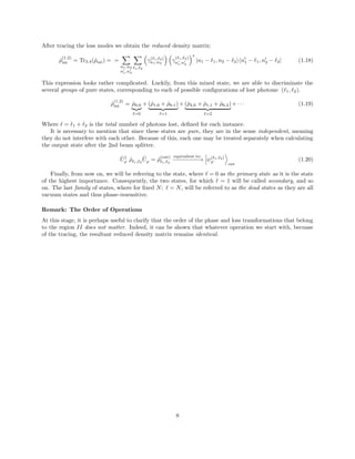
2.1.3 Between the SQL and the Heisenberg Limit
Both limits to interferometry are presented on the log-log plot (Fig. 2.1), which clearly shows us the potential
offered by quantum optics against the number of resource. Now, it is an important question: how we can
physically explore this region? In other words, which states of light and which detection strategy will allow
us to approach the Heisenberg limit or at least make it possible to go beyond the standard quantum limit?
As we will see, the answer for this question is not straightforward, especially if we consider lossy schemes.
Figure 2.1: The sensitivity scaling. N represents the number of photons used for a single trial and δϕ is the
sensitivity. The region between the SQL and the Heisenberg limit defines the phase super-sensitivity.
3Actually, since we work with the fixed total number of photons N, it is more adequate in this situation to refer to the
photon number-difference operator: ˆnab = ˆa†ˆa − ˆb†ˆb, where a and b refer to the two modes, respectively.
10](https://image.slidesharecdn.com/2d2c0242-172a-41b4-b64f-baad53159f08-160925145102/85/MSc_thesis_OlegZero-12-320.jpg)
![Remark on the Phase Super-Resolution
The phase super-sensitivity is often associated with another phenomenon: phase super-resolution. Since both
phenomena are often coexisting, it is important to distinguish between them. The phase super-sensitivity
is essentially a quantum phenomenon, which is related to the improvement in precision of measurements
(Fig. 2.1), if appropriate quantum states are used. Sometimes, it is accompanied with the so-called super-
resolution that is referred to as N-fold increment to the variation of interference fringes with ϕ (Ref. [2]). On
the other hand, phase super-resolution is not entirely a quantum property, as it has been alse demonstrated
for the coherent light (Ref. [12]).
2.2 Quantum Interference Measurement
In a classical measurement, what we basically detect is the output power in one or both of the interferometer
arms4
that brings us the information about the phase. In quantum measurements, however, we rather deal
with specific random outcomes or events and therefore we need statistical tools to be able to analyse the
output. In most general terms, the problem of current analysis can be recognised as the inference of an
unknown parameter (phase), based on the statistical data. This is the primary task for so-called Estimation
Theory. However, depending on the particular statistical representation of the problem, we can adapt either
the classical or quantum Estimation Theory.
In the next few sections, we shall briefly present the essence of both approaches in terms of their con-
straints and applicability. Based on that, we are going to agree on a common criterion for assessment for
the performance of the quantum states and optimisation.
2.2.1 Understanding the Output – The Estimation
First, let us now have a look at how to make the best possible accurate guess on the phase in the framework
of the classical statistics (Refs. [15, 16]).
Basic Assumptions of the Classical Estimation Theory
We assume that we deal with a set of mutually exclusive events Xi, belonging to the space of all events X.
This implies:
∀
Xi,j ∈X
p(Xi ∪ Xj) = p(Xi) + p(Xj) ⇐⇒ i = j (2.5)
where p(·) is the probability density function (pdf) defined for every event and thus:
p
i∈X
Xi =
i∈X
p (Xi) = 1 (2.6)
After perfoming M independent measurements (also called trials), we collect the data D, to be the following
set: D = {X
(1)
i , X
(2)
i , · · · , X
(m)
i , · · · , X
(M)
i }. The pdf defined for every event is conditioned on some unknown
(scalar5
) parameter p(Xi|θ); θ ∈ P ⊆ R and our aim is to infer its correct value. In order to make the
inference, we define an estimator6 ˇθ to be a decision rule, such that ˇθ = ˇθ(D, θ). Naturally, we demand our
estimator to be as accurate as possible.
4Of course, there exist several ways to do it. We can, for instance, detect the light emerging from one arm. We may also
detect power at both arms and then look at the difference, which “cleans” the signal from the background (classical) noise.
Nevertheless, the quantum (shot) noise will still remain the limitation in any case.
5In a most general case it is possible to have a vector of parameters. However, in this work, considering only one parameter
suffices.
6Estimators are ususally denoted as ˆθ. However, to distinguish them from quantum mechanical operators, they will be
denoted as ˇθ.
11](https://image.slidesharecdn.com/2d2c0242-172a-41b4-b64f-baad53159f08-160925145102/85/MSc_thesis_OlegZero-13-320.jpg)
![The Classical Fisher Information
The accurateness of an estimator is characterised by the mean square error:
mse(ˇθ) = (ˇθ − θ)2
= ˇθ2
− ˇθ 2
variance
+ ˇθ − θ
2
bias2
(2.7)
Note that, the mse expresses the deviation of the estimated value from the true value and hence it will later
‘fit’ to our definition of sensitivity.
If the estimator is unbiased, which means that the last term in (2.7) is zero and our estimate is right on
average, then the precision of the estimate is only limited by the variance. In such case the Cram´er-Rao
theorem applies:
var(ˇθ) ≥
1
I(θ)
(2.8)
I(ˇθ) is known as the classical Fisher information and it is the property of the mathematical model itself,
given by the following formula:
I(θ) =
∂ ln p(Xi|ϑ)
∂ϕ θ
2
X|θ
(2.9)
The symbol X|θ is used to remind us that the average should be taken over the space of events, not over the
parameter’s space P.
If the estimator efficient, which means if it is unbiased and has the ability to infer θ with the lowest possible
variance, then (2.8) becomes an equality. This situaltion is highly desirable, since with our estimator we
are not only able to extract the maximum possible information form the system, but we also gain a direct
correspondence between the Fisher information and the variance. Consequently, we may use I(θ) to find
the uncertainty.
In principle, efficient estimators are seldom found, or may not even exist at all, for certian problems.
Fortunately, for the purpose of interferometry, such estimators have been found and we shall see an example,
later on in this thesis. For now, the most important thing is to remember for which kind of problems or
models this appoach can be applied.
2.2.2 Quantum Estimation
In quantum mechanics, besides the classical uncertanty, our knowledge about the system is also limited
by the fact that quantum systems are described by an intrinsically statistical theory, which impose certain
restrictions to our measurements. According to this theory, we are only allowed to ‘look at’ those observables
that are represented by hermitian operators and if more than one observable is considered, their corresponding
operators are expected to commute, if the measurements are to be described by independent stochastical
distributions. Based upon these restrictions, the “old”, classical Estimation Theory has been deliberately
extended to its quantum successor.
In the contrary to its classical counterpart, this “upgraded” theory promises us more than how to make
a good estimate, but also, what is very important, it helps us to find a specific form of an operator that will
actually allow us to extract the maximal information out from the quantum system (Refs. [17, 18]). Let us,
therefore, have a quick look at what this theory offers.
The Basic Assumptions of the Quantum Estimation Theory
In quantum theory, the most general representation of a state is a density matrix, which belongs to a Hilbert
space ˆρ ∈ H. Here, the state is assumed to depend on some scalar7
, parameter ˆρ(θ); θ ∈ P ⊆ R. The
measurements are represented by a set of operators ˆΠi, whoose possible eigenvalues define the outcomes
7Similarly, the case analysed here is the single-variate case. In principle however, we may have a whole vector of parameters
θ = [θ1, θ2, ..., θN ].
12](https://image.slidesharecdn.com/2d2c0242-172a-41b4-b64f-baad53159f08-160925145102/85/MSc_thesis_OlegZero-14-320.jpg)
![X = {X1, X2, ..., Xi, ...}. If the operators commute, we can assign each estimator an operator ˇθ → ˆΘ,
such that ˆΘ|ˇθ = ˇθ|ˇθ . The state |ˇθ ∈ H(P)
belongs now to a space of all possible guesses and ˇθ has an
interpretation of an estimate. In other words, the measurement means that we operate ˆΘ on an eigenstate
|ˇθ and obtain the estimate ˇθ as a result. The joint conditional probability is defined as p(ˇθ|θ) = ˇθ|ˆρ(θ)|ˇθ ,
which is then used to minimise an associated cost function, analogically to minimising the rms in the classical
case.
Just as the density matrix is a generalised representation of a state, the POVM8
is the most general
form for the representing a measurement. In this case operators ˆΠi not need to commute and they are being
defined on every infinitesimal, disjoint sub-region of the parameter’s space ˆΠ(ˇθ; dˇθ); ˇθdˇθ ∈ P (Ref. [18]).
For an arbitrary interval of the parameter space ∆ ⊆ P, the POVM is found by:
ˆΠ(∆) =
∆
ˆΠ(ˇθ ; dˇθ ), (2.10)
with ˆΠ(P) = ˆ1. Note that this statement is the quantum mechanical analogy to the classical case (2.6). The
joint conditional probability is obtained by the trace:
p(ˇθ ∈ ∆|θ) = Tr ˆρ(θ)ˆΠ(∆) . (2.11)
This formula has an interprestation of the probability that our estimate ˇθ is found in ∆, when the system
is in ˆρ(θ). Only in the special case, when our measurement is a projective measurement, the operator (2.19)
becomes:
ˆΠ(∆) =
∆
|ˇθ ˇθ |dˇθ , (2.12)
where P
|ˇθ ˇθ |dˇθ = ˆ1.
The Quantum Fisher Information
Again, we would like to know how we could maximise the accuracy of our measurement. The definition of the
“quantum accuracy” is fortunately not much different from the classical one. If the measurement is unbiased,
which means that ˆΠ(ˇθ) ˆρ(θ) = θ then our estimate is correct on average and its accuracy is dictated by the
variance only:
var ˆΠ(ˇθ) =
P
ˇθ − ˆΠ(ˇθ) ˆρ(θ)
2
p(ˇθ|θ)dˇθ (2.13)
where p(ˇθ|θ)dˇθ = Tr[ˆρ(θ)ˆΠ(ˇθ; dˇθ)].
In this case, the quantum version of the Cram´er-Rao inequality becomes:
var ˆΠ(ˇθ) ≥
1
IQ(ˆρ(θ))
(2.14)
with IQ(ˆρ(θ)) to be recognised as the quantum Fisher Information.
With help of the so-called symmetric logarithmic derivative ˆL, that was introduced by Helstrom (Ref. [18])
and defined by the following relation:
∂ˆρ(θ)
∂θ
=
1
2
ˆLˆρ(θ) − ˆρ(θ)ˆL . (2.15)
We arrive at the formula for the quantum Fisher information:
IQ(ˆρ(θ)) = Tr ˆρ(θ)ˆL2
. (2.16)
8The POVM stands for the Positive-Valued Operator Measurement.
13](https://image.slidesharecdn.com/2d2c0242-172a-41b4-b64f-baad53159f08-160925145102/85/MSc_thesis_OlegZero-15-320.jpg)
![The matrix elements of ˆL can be computed by writing ˆρ(θ) in its eigenbasis and using eq. (2.15), according
to:
[ˆL]ij =
2
λi + λj
∂ˆρ(θ)
∂θ ij
(2.17)
The λi,(j) are the eigenvalues of ˆρ(θ) and whenever λi + λj = 0 we set [ˆL]ij = 0.
For now, the purpose of introducting these definitions may appear somewhat unclear or at least a little
bit out of the context. However, in just next few sections, we are going to see why it is so important to
understand the major assumptions of each of these two frameworks.
2.3 Criterion for Assessing the Performance
If we think of the Fisher information, classical or quantum, as of some sort intrinsic quantity of the system
whose extraction will determine the precision our measurement, it becomes natural to ask of which tools or
methods we need in order to be able to extract the maximum of it. An efficient estimator is the answer for
the classical case. The analogy existing in the quantum case is an appropriate POVM, also known as the
canonical measurement.
2.3.1 The Canonical Detection
What has been first showed by O. E. Brandorff-Nielsen and R.D. Gill (Ref. [19]) for pure states and then
extended by A. Luati (Ref. [20]) to mixed states is the following inequality:
var(ˇθ) ≥
1
I(θ)
≥
1
IQ(θ)
(2.18)
This chain clearly suggest that we should aim for extracting the quantum information. However, as just
mentioned before, this strategy requires the canonical measurement to saturate the quantum Cram´er-Rao
inequality (2.14). The specific form for such POVM has for long time been unknown, until it was first derived
by B.C. Sanders and G.J. Milburn (Ref. [21]). Adapting the Fock-state basis and setting the estimate to be
our phase shift ˇθ = ˇϕ, the form of this POVM (Ref. [5]) becomes:
ˆΠcan( ˇϕ) =
1
2π
| ˇϕ ˇϕ| , where: | ˇϕ =
N
n=0
ein ˇϕ
|n, N − n (2.19)
Unfortunately, the operator ˆΠcan( ˇϕ) must depend of what is to be measured and as also pointed out in the
Ref. [5]: “Except in special cases, it is not possible to perform canonical measurements with standard optical
equipment (photon counters and linear optical elements such as beam splitters)”.
Furthermore, the meaurement of this fom ‘works’ only, if the interferometer is lossless, which means our
output state is pure. As soon as even a tiniest loss is present in the system, our output results in a mixture of
many pure states as indicated in Chapter I. According to Ref. [3], in order to extract the maximum possible
information, we need one more piece of information about the system: we need to know exactly how many
of, and where, the photons were lost before applying the appropriate POVM. Such information will project
our density matrix onto one of the intrinsic pure states, which corresponds to a particular configuration of
loss ( a, b); ˆρout
Pr
−→ ˆρ
( a, b)
out . Only then we can apply the optimal POVM (2.19).
Except for the difficulty to realise the POVM, prior knowledge about the loss causes an even greater
technological issue. In each case, the requirement to know ( 1, 2) implies that we must measure the number
of photons at each branch without absobing them! Such measurement can be qualified as a quantum non-
demolition (QND) experiment, which although theoretically allowed, remains both practically undoable and
likely unfeasable for the forseeable future.
Since we are essentialy limited to using the “non-sophisticated” elements, such: beam splitters and photon
counting detectors, the important question arises: What are the limitations to our precision if using realistic
14](https://image.slidesharecdn.com/2d2c0242-172a-41b4-b64f-baad53159f08-160925145102/85/MSc_thesis_OlegZero-16-320.jpg)
![schemes? Can we still beat the SQL using photon counting detectors and ‘normal beam splitters’? If yes,
then how?
2.3.2 Realistic Detection
An example of a realistic setup such as the lossy Mach-Zehnder interferometer has just been introduced in
chapter I. Given the photon counters, we deal with the projective measurement in the Fock-state basis. Such
measurement can be represented by the operator:
ˆP = ˆa†
ˆa;ˆb†ˆb : ˆP|na, nb = (na, nb)|na, nb (2.20)
In this case, knowng the total number of photons N, we can still tell how many photons we have lost in
total, but we are given no information where the photons were lost. What is more, this measurement
strategy does not allow us to perform any adjustments during an act of a single measurement. Still we
assume our detector’s network has an idel recognition between the events: |2, 0 will not be confused with
|1, 0 , for instance, and the detector’s quantum efficiency is assumed to be unity – all loss is entirely in the
interferometer.
2.4 Efficiency vs Robustness
The direct consequence of the assumptions given in the previous section is that now, we arrive at classical
estimation. Indeed, according to Helstrom (Ref. [17, 18]) having non-optimal, but well-defined operator and
detection strategy, our estimation can be performed with the classical means.
2.4.1 Building the Estimator
First of all, let us define the space of events X. Upon the measurement (2.20), our outcomes are the
eigenvalues of the operator ˆP, which span the complete set XNph:
XNph =
0
n=N
n
k=0
(n − k, k) ≡
(N+2)(N+1)/2
i=1
Xi
(2.21)
The subscript Nph is used to remind us about the exact number of photons in one trial and the ‘reversed’
order of the first set-summation is a convention we use to indicate the ordering of the elements: (N, 0) ≡
X1, (N − 1, 1) ≡ X2 and so on.
The occurence of each one of Xi’s is determined by the conditional probability density function p(Xi|ϕ),
which also assumes an implicite dependence on loss and beam splitters’ strengths. The index i is used to
distinguish between every outcome in X and the pdf’s can be calculated from the output density matrix
ˆρout(ϕ).
Based on the so-called Bayesian approach, we look for the posterior probabiliy p( ˇϕ|D) = p( ˇϕ|
M
m=1 X
(m)
i ),
which is the probability of having the phase shift ϕ conditioned on all outcomes collected throughout mea-
surement process. According to Bayes’ theorem:
p( ˇϕ|D) =
p( ˇϕ)p(D| ˇϕ)
p(D)
(2.22)
p( ˇϕ) is the so-called prior probability distribution, which corresponds to our knowledge about the phase
before any measurement is done. If nothing is known about the phase a priori, then p( ˇϕ) = 1/2π. The
denominator is the a priori knowledge about the data and it is to act as the normalisation constant p(D) =
P
p( ˇϕ )p( ˇϕ |D)d ˇϕ . Finally, our parameter subspace is usually P ≡ [−π, π].
15](https://image.slidesharecdn.com/2d2c0242-172a-41b4-b64f-baad53159f08-160925145102/85/MSc_thesis_OlegZero-17-320.jpg)
![When the number of measuremets is large M 1, then by virtue of the Central Limit Theorem, the
equation (2.22) becomes Gaussian and according to Ref. [2], it can be approximated by:
p( ˇϕ|D) ≈ p( ˇϕ|ϕ) =
1
N
i∈X
p(i| ˇϕ)Mp(i|ϕ)
(2.23)
Where N = P i∈X p(i| ˇϕ )Mp(i|ϕ)
d ˇϕ is the normalisation constant. Equation (2.23) is the Maximum
Likelihood Estimatior (MLE). Indeed, this function tells us how likely it is that our guess ˇϕ matches the true
phase shift ϕ.
By analysing the derivatives, it is proven in Ref. [2] that this function attains maximum when ˇϕ = ϕ and
its width is equal to the variance. This means that in the asymphotic limit we have obtained the efficient
estimator and therefore, we may use the (classical) Fisher information to optimise our system.
Remark on Phase Ambiguities
Last, but not least, it may happen that the likelihood function (2.23) possesses more than one maximum. If
such situation happens, we face an ambiguity in recognising the phase, which is similar to super-resolution.
This is, fortunately, a minor problem, since according to Ref. [5], a possible implementation of a feedback
loop9
to the system or changing the input states from trial to trial will naturally solve the ambiguity, by
concentrating the likelihood function around the true value.
2.4.2 The N00N State
Before moving on to the next chapter to see how we can optimise the system, let us have a closer look at
one, very specific example: the so-called N00N state:
|N00N =
1
√
2
|N, 0 + eiχ
|0, N ; χ ∈ R (2.24)
The name of this state is self-explanatory. If we look at its form, we quickly realise, why this state has
been typed a good candidate for quantum interferometry. Indeed, if this state is the interferometer’s internal
state, it will ‘pick-up’ the maximum possible phase shift (see eq. (1.5)), in principle, allowing us to perform
measurements exactly at the Heisenberg limit.
However, as soon as there exists loss in our system, loosing only one photon will cause a total decoherence
of the system, degrading the state to a mixtrue that will exhibit no interference at all. To show this, let us
define a one-photon loss operator ˆPη = [|N − 1 N| ⊗ ˆ1] ⊗ [|1 0| ⊗ ˆ1]loss and see what happens to the N00N
state:
ˆPη|N00N =
1
√
2
|N − 1, 0 ⊗ |1, 0 loss (2.25)
Under trace, we will discard the phase-information together with the loss-modes |1, 0 loss and our new state
|N − 1, 0 will have no “partner” to interfere with.
2.4.3 Robust States
We have just seen how fragile the N00N states are, even though their sensitivity to phase, is the highest
possible. In practice losses will always occur and depending on each partiular case, there will be other states,
whose sensitivity, although not as high, will be compensated by robustness.
In the next chapter will shall see in more detail, which states are best for each case and how they are
found.
9Such (electronic) feedback would possible re-adjust the auxiliary phase shift Φ placed at the second arm, after each trial.
16](https://image.slidesharecdn.com/2d2c0242-172a-41b4-b64f-baad53159f08-160925145102/85/MSc_thesis_OlegZero-18-320.jpg)
![Chapter 3
Searching for the Optimum
We have finally gathered all tools needed to understand and correctly interpret all possible experimental
outcomes. Now, we can use this knowledge to optimise the perfomance of our interferometer. As discussed
in Section 2.4.1, the Bayesian estimator provides us the method to recognise the phase shift, whereas its ap-
proximation, the MLE, becomes the efficient estimator in the asymtotic limit. Consequently, by maximising
the Fisher information we immediately learn about the optimal performance.
3.1 Global Strategy
As a first step, we should consider the global strategy, which means how we should proceed with our mea-
surement in general. As presented in Fig. (2.1), the best precision allowed by physics is the Heisenberg
limit. However, it is only attainable in the absence of loss, if the N00N or similar states are used (Ref. [2]).
Essentially, the higher the number of photons N is used in a single trial, the more “beneficial” the measure-
ment becomes. On the other hand, as N is being increased, it not only becomes much more cumbersome
to prepare such state, and later, to appropriately detect its outcomes, but also the amount of loss we can
tolerate quickly decreases.
3.1.1 The Problem of Loss
This fact can easily be demonstrated if we equate the sensitivity of the N00N state (Ref. [3]) with the one
of the coherent state:
δϕSQL = δϕN00N ⇐⇒
1
√
Nη
=
1
N ηN
=⇒ η(N) = N
1
1−N . (3.1)
Setting ¯N = Nη for the coherent state and transforming the equation (3.1), we obtain the function η(N) that
tells us the minumum tolerable transmission, below which the N00N state performs worse than the classical
light. For example, if using a 100-photon N00N state, we must ensure that: η > 95% and if N = 103
, then
η > 99%. This shows that the improvement promissed by the quantum light is greatly inhibited, even if
disarding any other source of error.
3.1.2 The Problem with Implementation
In reality, besides the loss, one must also consider the technological drawbacks. Although these are greatly
excluded from current discussion, one should be aware of the two important issues which originate from the
technological side: The first one is the experimental cost of preparing the input state. And the second one is
to guarantee the low error-rate detection of the outcomes. Both of these issues put further bounds to the
maximum number of photons which we can afford to use in any one trial.
17](https://image.slidesharecdn.com/2d2c0242-172a-41b4-b64f-baad53159f08-160925145102/85/MSc_thesis_OlegZero-19-320.jpg)
![3.1.3 Possible Solutions
Primarly, we could ask why not replacing a high-N-photon state with more states of lower N and increase
the number of repetitions m? Indeed, this is the exactly how the measurement is conducted in practice.
However, as each trial is purely independent, the Fisher information becomes additive, which leaves us with
the classical scaling against the number of trials: δϕ ∝ m−1/2
.
Until now, no phase super-sensitivity has been experimentally demonstated using states of more than
N = 4 photons (Ref. [6, 7]). Still, the experimental realisation in Ref. [6] was conducted in the so-called
post-selecton paradigm1
, which may be regarded as an approximation to canonical measurements, since the
inference is based only on the “successful events”. However, when certain “undesired” outcomes are dismissed
a posteriori, the exact number of resources needed for certain precision becomes undefined, thus not showing
us the true sensitivity limit.
Another method proposed, was to make a single photon pass though the phase shifter several times
(Ref. [7]), which results in a phase-shift proportional to the number of bounces. Nevertheless, the analogical
solutions are also known in the classical interferometry2
, where the presence of a high-finesse cavity enhances
the precision. It will, therefore, be more appropriate to refer the quantum multipass interferometry to its
classical counterpart and let the super-sensitivity itself be discussed agreeing on a most fundamental setup.
3.2 Preliminary Assumptions for Optimisation
Taking all these facts into account, the following work was focused on optimising the low-N-photon states in
the context of loss (N = 2, 3). Concerning the loss, two important situations have been treated explicitely:
• the symmetric loss: η = [η1, η2] ≡ η, which is the model for the loss existing equally in both arms
• and the asymmetric loss: η = [η, 1], which could be the model for a lossy phase shifter or sample
In every case, the coupling strenth of both beam splitters has been set symmetric: ξ = [ξ1, ξ2] ≡ 1/2, unless
stated otherwise.
The optimisation algorithm was implemented using the Wolfram Mathematica 7.0 software. For
this purpose, the classical (and discrete) Fisher information (2.9)
I(ϕ0) =
i∈X
1
p(Xi|ϕ)
∂p(Xi|ϕ)
∂ϕ ϕ0
2
(3.2)
has been rearranged for the purpose of computation:
I(ϕ0) =
i∈X
p(Xi|ϕ0)
p(Xi|ϕ0 + ∆ϕ)
p(Xi|ϕ0)∆ϕ
−
1
∆ϕ
2
. (3.3)
The ϕ0 is the phase at which we bias our interferometer3
. For sufficiently small step (∆ϕ = 10−6
), the
simulation results show that the Fisher information is independent from the value of ϕ0. Except for ϕ0 = 0,
it can be set to an arbitrary value.
1The post-selection paradigm is also known as the adaptive measurements. We could agree, for instance, on rejecting every
event, in which we know we have lost photons. This procedure, will obviously increase the overall precision, but the exact
number of photons remains undefined.
2For instance: the Fabry-P´erot or Fizeau interferometers.
3It is in any way related to the estimator bias, which is equal to zero for efficient estimators.
18](https://image.slidesharecdn.com/2d2c0242-172a-41b4-b64f-baad53159f08-160925145102/85/MSc_thesis_OlegZero-20-320.jpg)
![3.2.1 2-photon State Modelling
Let us assume we have an arbitrary 2-photon input state:
|ψ in = x2,0|2, 0 + x1,1|1, 1 + x0,2|0, 2 , x0,2, x1,1, x0,2 ∈ C. (3.4)
After all transformations discussed in Chapter I, we arrive at the output density matrix ˆρout(ϕ), from we can
discriminate six pure states, whose components’ complex amplitudes are: y
( 1, 2)
na,nb (ϕ), with na, nb referring to
the number of photons and ( 1, 2) specifying the particular loss instance. The probability associated with
each component can be calculated taking p
( 1, 2)
na,nb (ϕ) = |y
( 1, 2)
na,nb (ϕ)|2
.
Accounting for the measurement operator (2.20), our space of all possible measurement outcomes reads:
X2ph = {(2, 0), (1, 1), (0, 2); (1, 0), (0, 1); (0, 0)} ≡
6
i=1
Xi . (3.5)
It is essential to note that certain outcomes, i.e. the outcome: (1, 0) can be obtained loosing one photon
in either of the arms. Since we have no means to monitor the lost photon, these two situations become
indistinguishable. On the other hand, we also know they are mutually exlusive, hence (2.5) applies and we
must add the probabilities
p(X4|ϕ) ≡ p((1, 0)|ϕ) = p
(1,0)
1,0 (ϕ) + p
(0,1)
1,0 (ϕ), (3.6)
before puting them to (3.2). Similar situation happens for all other indistinguishable, mutually exclusive
events, not only in the case of 2-photon states.
3.2.2 3-photon State Modelling
For the 3-photon case, we assume to have an arbitrary 3-photon input state:
|ψ in =
3
k=0
x3−k,k|3 − k, k , ∀k x3−k,k ∈ C. (3.7)
Again, all transformations discussed in Chapter I apply, but this time, our outcome space X3ph contains
more events:
X3ph =
0
n=3
n
k=0
(n − k, k) ≡
10
i=1
Xi . (3.8)
All other procedures remain the same, as before.
3.2.3 The Implementation (Fock States)
Now, the task is to search for such input amplitudes x2ph = [x2,0, x1,1, x0,2] (or x3ph = [x3,0, x2,1, x1,2, x0,3]),
so that I is maximised. For this purpose, we parametrise the input state with i, ∈ Ri, ζi ∈ Zi; i = 1, 2, (3)
as follows:
|ψI 2ph = cos 1|2, 0 + eiζ1
sin 1 cos 2|1, 1 + eiζ2
sin 1 sin 2|0, 2 , (3.9)
|ψI 3ph = cos 1|3, 0 + eiζ1
sin 1 cos 2|2, 1
+ eiζ2
sin 1 sin 2 cos 3|1, 2 + eiζ3
sin 1 sin 2 sin 3|0, 3 . (3.10)
The parametrisation in (3.9) and (3.10) ensures the normalisation. The parameter space, defined to be
BN=2,(3)
def
=
i=1,2,(3)
Ri
⊕
i=1,2,(3)
Zi
⊆ R4,(6)
, (3.11)
19](https://image.slidesharecdn.com/2d2c0242-172a-41b4-b64f-baad53159f08-160925145102/85/MSc_thesis_OlegZero-21-320.jpg)
![can further be limited to Ri = [0, π/2]; Zi = [0, 2π); i = 1, 2, (3) in order to reduce the computation time.
Finally, the simulation is run and for each value of η, the state giving the highest I is found and I is plotted
against η (the symmetric case) or µ (the asymmetric case, see later).
Remark on the Parameter Space Sampling
In order to reduce the computation time even further, the space B is sampled, usually taking 5 points
from each Ri and 4 points from each Zi’s. Consequently, we find an approximation to the maximal Fisher
information, which is, nevertheless, a good approximation, since increasing the number of samples4
in B
leads to a difference no higher than 12% with the respect to the previously obtained value of I. For clarity,
we shall refer to the number of samples as s ≡ (s 1
.s 2
.(s 3
).sζ1
.sζ2
.(sζ3
)), when later discussing the results.
Remark on the Asymmetry Treatment
When the losses are symmetric, by definition η may be interpreted as the overall interferometer’s transmis-
sion. This is not exactly true, when the loss becomes asymmetric. According to Ref. [8], the influence of
the asymmetry can be treated by adjusting the coupling strength of the first beam splitter ξ1:
ξ1 =
1
η + 1
. (3.12)
If ξ1 is adjusted as indicated above, the visibility of the classical signal can be restored. However, in this
case, the overall transmittivity can be expressed in more intuitive way. Let us introduce a new variable µ,
which we will call an efficiency:
Ψ = (ξ1η)Ψ + (1 − ξ1)Ψ
(3.12)
=
2η
1 + η
Ψ
def.
= µΨ. (3.13)
Where Ψ be an input power injected to the first arm and Ψ = µΨ is the output. Now, we have a coefficient
that is expresses the loss in manner that is independent from the asymmetry – “output/input”.
3.2.4 Coherent State Modelling
When discussing the improvement, the SQL provides us a natural reference point. Let us, therefore, briefly
ilustrate how the coherent state is accounted in our simulation.
Since any coherent state modes are perfectly uncorrelated, given |ψcoh
in = |α, 0 injected as the input, the
output state is easily found by repeting all previous transformations:
ψcoh
out (ϕ) = αe−iϕ
η1ξ1ξ2 − α η2(1 − ξ1)(1 − ξ2)
⊗ αe−iϕ
η2ξ1(1 − ξ2) + α η2(1 − ξ1)ξ2 = βa, βb . (3.14)
Accounting for (1.2), the probability of detecting k-photons in output modes a, b is:
p(k|βa,b) = e−|βa,b|2 |βa,b|2k
k!
. (3.15)
Since |α|2
has the interpretation of the photon number average ¯N, and since in our case only ¯N = 2, 3 photon
states are considered, (3.2) can be well-approximated, by taking only first ten terms of (3.15)
I
(coh)
a,b (ϕ0) =
10
k=0
1
p(k|βa,b)
∂p(k|βa,b)
∂ϕ ϕ0
2
. (3.16)
4Increasing the number of samples from (5.5.4.4) → (5.5.8.8) in the 2-photon symmetric case shows no resolvable difference
between the results. In the asymmetric case, the same increment leads to 12% for µ = 0.62, which is the highest difference occur-
ing between the two solutions. Further increasing of the sampling density shows that the solution is converging. Unfortunately,
due to the limited computational power of the computer, the convergence of the 3-photon as not investigated.
20](https://image.slidesharecdn.com/2d2c0242-172a-41b4-b64f-baad53159f08-160925145102/85/MSc_thesis_OlegZero-22-320.jpg)
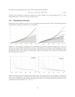
![Figure 3.3: The sensitivity of 3-photon states against losses. Left: the symmetric case (η), Right: the asymmetric
case (µ). The dark-blue dots: the optimal states with (5.5.5.4.4.4) assuming the input amplitudes complex xin ∈ C;
the bright-blue dots: the optimal state with (5.5.5.1.1.1), but fixing all amplitudes real xin ∈ R; the red line: the
N00N state, the gray line: the coherent state with ξ1 = 1/2; the black line: the coherent state with optimally adjusted
beam splitter: ξ1 = 1/(1 + η).
3.3.1 Discussion
The 2-photon Case
The optimisation algorithm shows the existance of several input states, whose sensitivity dominates the
sensitivity of all the other input states within specific regions of loss (Fig. 3.1). The selected optimal
states are essentially different in each case (symmetric/asymmetric loss), exept for in the two extreme cases:
x0 = [1, 0, 0] and xN00N = [1, 0, 1] /
√
2. The latter input state corresponds to the internal N00N state
(also achievable with [0, 1, 0]-input), which has been introduced in Section 2.4.2 as yielding the highest
sensitivity. From Fig. 3.2, we can observe that the N00N state is selected ‘best’ in the low-loss regime:
ηN00N,2 ≥ 0.65 (symmetric) and µN00N,2 ≥ 0.96 (asymmetric), attaining the highest Fisher information
I = 4 if the interferometer is ideal. Shortly after reaching the threshold (ηN00N,2 or µN00N,2), its performance
gets quickly degraded, which stands in agreement with Refs. [3, 9, 10], (see also eq. (3.1)). The existance
of such high threshold given for the N00N state in the asymmetric case can be explained with the fact, that
the N00N state is a symmetric state itself, hence might naturally be less tolerant to losses that are present
only in one arm.
Below ηN00N,2 (or µN00N,2), more robust states of lower sensitivity are found. And for extremely high
losses η < 0.13 (and µ < 0.11), the x0 state becomes the optimum. Its sensitivity, in the symmetric case,
coincides perfectly with the SQL-line, signifying the classical performance. In the asymmetric case, the state
performs slightly better.
The 3-photon Case
First of all, the results obtained in this case indicate ‘a proper’ scaling of the Fisher information5
against
the number of photons N. In either case (symmetric and asymmetric), when no loss is present, the Fisher
information for the N00N state grows quadratically, whereas it remains linear for the coherent state. What
is more, when losses are present Icoh is also linear vs. η or µ, provided that ξ1 is optimally adjusted.
Most of the conclusions formulated for the 2-photon case ar also valid when N = 3, except for the fact,
that a slightly different state (other than x0 = [1, 0, 0, 0]) is preferred in the high-loss regime, when the
loss exists in one arm only. Similarly to when N = 2, the N00N state performs best when losses are low,
although its regime is now bounded by new thresholds: ηN00N,3 ≥ 0.74 or µN00N,3 ≥ 0.83. Surprisingly, the
region of the N00N state extands further, comparing to the previous situation, if the loss is asymmetric. The
5...and hence the uncertanty, since δϕ = 1/ I(ϕ) when saturating the Cram´er-Rao bound.
22](https://image.slidesharecdn.com/2d2c0242-172a-41b4-b64f-baad53159f08-160925145102/85/MSc_thesis_OlegZero-24-320.jpg)
![possible explanation6
to this fact could be that if N is set odd, there exists no |N/2, N/2 component inside
the interferometer and therefore, it might somehow be easier for the odd-numbered N00N states to resist
asymmetries.
Finally, we should emphasise the importance of assuming the input amplitudes complex, before proceeding
with the optimisation. As we can see on Fig. 3.3 (right), when the amplitudes are constrained real, the space
B is being greatly reduced (dim B = 4, (6) → 2, (3)) and the “optimal” states then found may even exhibit
sensitivity lower than that of the coherent state.
3.4 The Confirmation of the Method
As stated in the Introduction, all optimisation methods developed to investigate the influence of photon-
loss, which I was aware of throughout the whole time of my thesis work, were entirely based on the quantum
Fisher information (Refs. [3, 9, 10]), thus, as discussed in Chapter II, not revealing us the realistic limit to
the sensitivity of interferometers. The motivation for my work, therefore, was to find the sensitivity limit
assuming a more implementable setup, which I have found by extanding the idea of H. Uys and P. Meystre
(Ref. [2]) and choosing the classical Fisher information to build my algorithms upon.
In the paper published in December 2009 by Lee, et al. (Ref. [4]), the authors proceed with the same
reasoning and even extanding their algorithms to account for an arbitrary number of photons. Unfortunately,
I have learnt about this publication too late in order to start my work anew and try to explore the unexplored,
as I was already at the stage of summerising my results. The same publication has, on the other hand, granted
me a great privilage and opportunity to confront my results, at least partially, with the work done by the
scientists. Figure 3.4 presents a “common case”, which is used for the comparison:
Figure 3.4: The sensitivity vs. the number of photons N used in one trial, for the loss-asymmetric case. This
figure is the part of research conductd by Lee et al. (Ref. [4]). The markers with the numbers correspond to the
data obtained by me and they are used for the comparison. The black numbers: the 2-photon case, the green-bold
numbers: the 3-photon case.
As we can observe from the Fig. 3.4, the position of the points calculated by me, match exactly the
positions calculatd by Lee, et al. for the same points. Consequently, I take this agreement anyhow gives me
a feeling of confidence that I was, indeed, on the right track.
6This is purely a hypothesis which requires verifictaion.
23](https://image.slidesharecdn.com/2d2c0242-172a-41b4-b64f-baad53159f08-160925145102/85/MSc_thesis_OlegZero-25-320.jpg)
![3.5 If Accessing the Inaccessible...
Finally, the publication by Lee, et al. has encouraged7
me to investigate just one more case.
In Chapter II, when discussing the optimal measurement strategy, we mentioned that whenever the
interferometer is lossy, the output state results in a mixture and the only ‘possibility’ for us to be able to
perform the optimal measurements, is to somehow monitor the losses. It was also emphasised that such
monitoring is practically impossible to construct. However, it is still interesting from the theoretical point
of view, to see of what impact this information might have on the interferometer’s precision.
Loss Monitoring and Distinguishability of Events
Let I(Xi) be one of the terms of the sum I(X) = i I(Xi) (eq. (3.2)), corresponding to a particular
experimental outcome Xi that is a result of the occurence of ˜Xi,1 and ˜Xi,2. It was indicated in section 3.2.1
that if ˜Xi,1 and ˜Xi,2 are mutually exclusive, indistinguishable events (2.5), we should add their probability
functions and calculate the Fisher information (3.2) that is based on their sum:
I(Xi) = I ˜Xi,1 ∪ ˜Xi,2 (3.18)
Assuming now that we are able to monitor the loss, the events ˜Xi,1 and ˜Xi,2 are still mutually exclusive,
but now, they become distinguishable. Since the Fisher information is calculated for the visible outcomes,
we have:
˜I(Xi) = I ˜Xi,1 + I ˜Xi,2 (3.19)
In general, we expect: ˜I(Xi) = I(Xi), which implies that depending on the distinguishability of events, we
will arrive at different Fisher information in each case. The question now arises: How large the difference
would be: ∆I = |I(X) − ˜I(X)|?
Due to the large number of degrees of freedom, even for N = 2 the answer seems to be rather difficult
to find analytically. However, inspecting the formula (3.2), we see that the Fisher information depends on
the derivatives of each pdf with the respect to the phase p (Xi|ϕ). What is more, each derivative is squared,
which makes I independent from sing of p (Xi|ϕ). Therefore, we expect that if a certain state is found, such
that under losses, it ‘creates’ two events of the opposite probability slopes, then depending on wheather we
calculate the Fisher information according to (3.18) or (3.19), we should arrive at ∆I = 0.
The epsilon-State
Let us consider a 2-photon state. Particularly, let us concentrate on two loss-origined events:
|1, 0 (⊗|1, 0 loss) ≡ ˜X4,1 (3.20)
|1, 0 (⊗|0, 1 loss) ≡ ˜X4,2 (3.21)
The event (1, 0) ≡ X4 = ˜X4,1 ∪ ˜X4,2 is the observable outcome corresponding to |1, 0 output state.
Now, let us consider an example to be the ε-state, defined as the following input state:
|ψI(ε) =
1
√
2
eiε
|2, 0 + |0, 2 (3.22)
Setting ε = π/2 we obtain a state, whose output pdf’s p
(1,0)
1,0 (ϕ) and p
(0,1)
1,0 (ϕ) are equal in amplitude, but
being exactly out-of-phase. Hence:
p(X4|ϕ) = p
(1,0)
1,0 (ϕ) + p
(0,1)
1,0 (ϕ) = const. (3.23)
7The reason for undergoing this investigation was due to my initial misinterpretation of their paper. I have, basically,
misunderstood the notation used by the authors and hence postulated that they have not accounted for the fact that certain
experimental outcomes apear indistinguishable to us. I was wrong. Nevertheless, I have decided to include these results as, in
my opinion, it still might be interesting to observe of what happens if we are able to monitor the losses (as implicitely assumed
in Ref. [8]).
24](https://image.slidesharecdn.com/2d2c0242-172a-41b4-b64f-baad53159f08-160925145102/85/MSc_thesis_OlegZero-26-320.jpg)
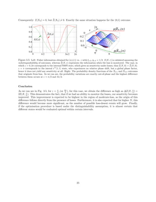
![Discussion
Two major tasks have been realised in this work. First of all, two existing statistical methods were com-
pared and evaluated, focusing strongly on their applicablility when it comes to practically implementable
measurements and accessible quantum information. Next, agreeing on a common criterion, the sensitivity
limits were investigated assuming photon losses, existing equally in one or both interferometer’s arms. By
developing a computer algorithm, the optimal quantum states were found in each case, assuming both the
existance of realisable measurement schemes and no adaptive measurements for N = 2, 3 photon states. In
principle the method could be extended to an abitrary photon number N, however the needed computing
resources would grow exponentially with N. Furthermore, the correctness of the method was (partially)
confirmed by comparing the results to Lee, et al. (Ref. [4]) and finally, it is shown that the difference up
to 200% in Fisher infomation is possible, if the specific information of the photon loss is known prior to the
measurement.
What is important to mention is that the optimisation method discussed in Chapter II, is approximate
due to the long time needed for computation. Therefore, its precision, in principle, is not expected to
increase if the number of photons N is increased. In cases of higher N’s, global optimisation algorithms
should be implemented or the density of sampling of B increased accordingly. Nevertheless, since in any
realistic situation N is low, this method gives a correct assessment of the sensitivity limit.
Last, but not least, concerning the scope of this work and its contribution to science, the limits to the
phase sensitivity were found with a strong focus on practcally realisable systems. Still, the experimental
cost of “producing” the quantum states on demand and non-ideal detection schemes existing remain most
important technological challanges for the fututre. Therefore, as a forecast, accounting for the effect of these
two problems in the mathematical model, would probably be the next step in the current analysis that
should bring us closer to the truth.
26](https://image.slidesharecdn.com/2d2c0242-172a-41b4-b64f-baad53159f08-160925145102/85/MSc_thesis_OlegZero-28-320.jpg)
![Bibliography
[1] Gunnar Bj¨ork and Jonas S¨oderholm:
“The Dirac-notation in quantum optics”,
ICT Department, KTH Electrum 229 S-164 40 Kista, Sweden,
corse notes, (2005).
[2] H. Uys and P. Meystre:
“Quantum states for Heisenberg-limited interferometry”
Physical Review A 76, 013804 (2007).
[3] R. Demkowicz-Dobrza´nski, U. Dorner, B. J. Smith, J. S. Laudeen,
W. Wasilewski, K. Banaszek and I. A. Walmsley:
“Quantum phase estimation with lossy interferometers”
Physical Review Letters, 102, 040403, (2009).
[4] T. W. Lee, S. D. Huver, H. Lee, L. Kaplan, S. B. McCracken, C. Min, D. B. Uskov, C. F. Wildfeuer,
G. Veronis and J. P. Dowling:
“Optimization of quantum interferometric metrological sensors in the presence of photon loss”
Physical Rewiev A 80, 063803 (2009).
[5] D. W. Berry, B. L. Higgins, S. D. Bartlett, M. W. Mitchell,
G. J. Pryde and H. M. Wiseman:
“How to perform the most accurate possible phase measurements”
Physical Review A 80, 052114 (2009).
[6] R. Okamoto, H. F. Hofmann, T. Nagata, J. L. OBrien,
K. Sasaki and S. Takeuch:
“Beating the standard quantum limit: phase super-sensitivity of N-photon interferometry”
New Journal of Physics 10, 0703033 (2008).
[7] B. L. Higgins, D. W. Berry, S. D. Bartlett, M. W. Mitchell,
H. M. Wiseman, G. J. Pryde:
“Demonstrating Heisenberg-limited unambiguous phase estimation without adaptive measurements”
New Journal of Physics 11, (2009).
[8] M. Kacprowicz, R. Demkowicz-Dobrza´nski, W. Wasilewski, K. Banaszek and I. A. Walmsley:
“Experimental quantum-enhanced estimation of a lossy phase shift”
arXiv:0906.3511v1, (2009).
[9] U. Dornier, R. Demkowicz-Dobrza´nski, B. J. Smith, J. S. Lundeen,
W. Wasilewski, K. Banaszek and I. A. Walmsley:
“Optimal quantum phase estimation”
Physical Review Letters 102, 040403 (2009).
[10] R. Demkowicz-Dobrza´nski, U. Dorner, B. J. Smith, J. S. Lundeen,
W. Wasilewski, K. Banaszek and I. A. Walmsley:
“Quantum phase estimation with lossy interferometers”
Physical Review A 80, 013825 (2009).
27](https://image.slidesharecdn.com/2d2c0242-172a-41b4-b64f-baad53159f08-160925145102/85/MSc_thesis_OlegZero-29-320.jpg)
![[11] T. Kim, J. Shin, Y. Ha, H. Kim, G. Park, T. G. Noh, C. K. Hong:
“The phase-sensitivity of a Mach-Zehnder interferometer
for the Fock state inputs”
Optical Communications, 156, 37-42, (1998).
[12] Ch. Kothe, G. Bj¨ork and M. Bourennane:
“Arbitrarly High Super-Resolving Phase Measurements at Telecommunication Wavelengths”
arXiv:1004.3414v1, (2009).
[13] P. Hariharan:
“Optical Interferometry”
Elsevier Science (USA), 2nd Edition (2003),
p.: 246–248 and p.: –
[14] Hans-A. Bachor and Timothy C. Ralph:
“A Guide to Experiments in Quantum Optics”
Wiley-VCH, 2nd Edition (2003),
p.: 117–119.
[15] Liam Paninski:
“Introduction to Mathematical Statistics”
http://www.stat.columbia.edu/˜liam/teaching/4107-fall05/index.html
course notes for Statistical Inference, Columbia University, (2005).
[16] Roberto Togneri:
”Estimation Theory for Engineers”
http://www.ee.uwa.edu.au/˜roberto/teach/Estimation Theory.pdf
The University of Western Australia, (2005).
[17] C. W. Helstrom:
“Quantum Detection and Estimation Theory”
Journal of Statistical Physics, Vol. 1, No. 2 (1969).
[18] C. W. Helstrom:
“Cram´er–Rao Inequalities for Operator-Valued Measures in Quantum Mechanics”
International Journal of Theoretical Physics, Vol. 8, No. 5 (1973).
[19] O. E. Brandorff-Nielsen and R. D. Gill:
“Fisher Information in Quantum Statistics”
J. Phys. A: Math. Gen. 33, 4481–4490 (2000).
[20] A. Luati:
“Maximum Fisher Information in Mixed State Quantum Systems”
The Annals of Statistics, 32, 1770–1779 (2004).
[21] B. C. Sanders and G. J. Milburn:
“Optimal Measurements for Phase Estimation”
Physical Review Letters, 75, 2944 (1995).
[22] Z. Hradil, R. Myˇska, J. Peˇrina, M. Zawisky, Y. Hasegawa and H. Rauch:
“Quantum Phase in Interferometry
Physical Review Letters, 76, 4295–4298, (1996).
[23] M. Zawisky, Y. Hasegawa, H Rauch, Z. Hradil, R. Myˇska and J Peˇrina:
“Phase Estimation in Interferometry”
J. Phys. A: Math. Gen 31, 551–564, (1998).
28](https://image.slidesharecdn.com/2d2c0242-172a-41b4-b64f-baad53159f08-160925145102/85/MSc_thesis_OlegZero-30-320.jpg)
![[24] Leslie E. Balentine:
“Quantum Mechanics a Modern Development”
Simon Fraser University,
World Sicentific Pbs. (1998).
others:
[25] Stephen Wolfram:
“The Mathematica Book”
Wolfram Media, Cambridge Univ. Press,
3rd Edition, (1996).
[26] Wikibooks: “LATEX”
http://en.wikibooks.org/wiki/LaTeX
[27] Art of Problem Solving:
http://www.artofproblemsolving.com/Wiki/index.php/LaTeX
29](https://image.slidesharecdn.com/2d2c0242-172a-41b4-b64f-baad53159f08-160925145102/85/MSc_thesis_OlegZero-31-320.jpg)