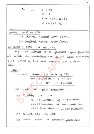
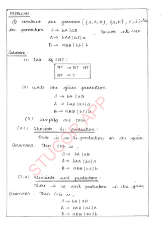
The document provides an introduction to automata theory and formal languages, highlighting their significance in computing and proofs of computability. It categorizes languages into various types recognized by different automata and discusses the mathematical foundations of these concepts. Additionally, it covers the methodology of formal proofs and different forms of reasoning used in programming and mathematical logic.
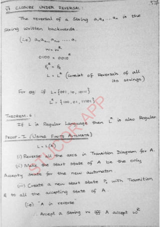
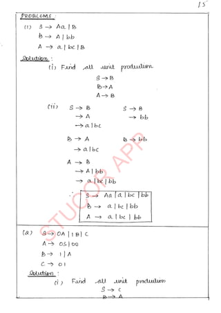
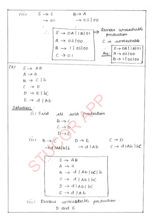
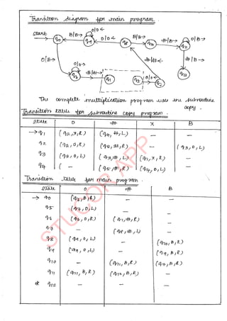
![1.17
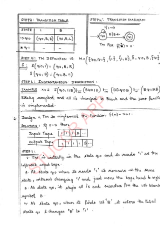
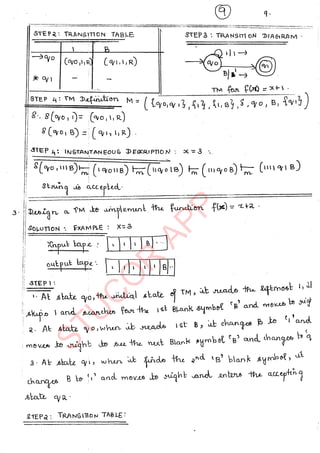
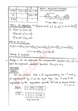
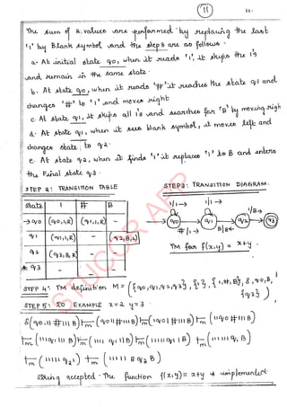
Automata Fundamentals
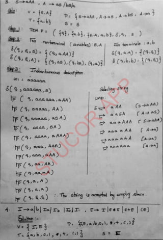
Induction
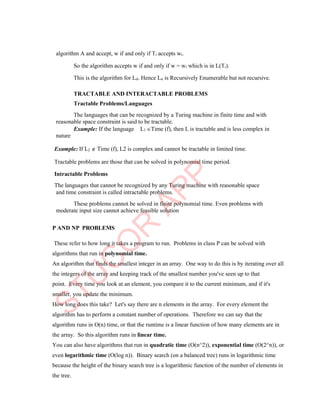
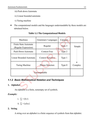
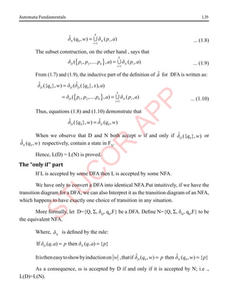
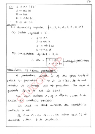
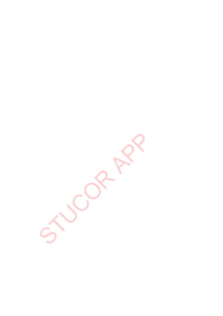
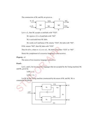
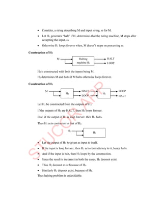
Let T be a tree built by the inductive step of the definition, from root node N and k
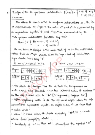
smaller trees T1
, T2
,..., Tk
. We may assume that the statements S(Ti ) hold for i = 1, 2,...,
k. That is, let Ti
have ni
nodes and ei
edges; then ni
= ei
+ 1.
The nodes of T are node N and all the nodes of the Ti
’s. There are thus 1 + n1
+ n2
+....+ nk
nodes in T. The edges of T are the k edges we added explicitly in the inductive
definition step, plus the edges of the Ti
’s.
Hence, T has k + el
+ e2
+ …. + ek
edges ... (1.3)
If we substitute ei
+ 1 for ni in the count of the number of nodes of T we find that
T has 1 + [el
+ 1] + [e2
+ 1] + …. + [ek
+ 1] nodes ... (1.4)
Since there are k terms in (1.3), we can regroup (1.4) as
k + 1 + el
+ e2
+ …. + ek ... (1.5)
This expression is exactly 1 more than the expression (1.3) that was given for the
number of edges of T. Thus, T has one more node than it has edges.
Theorem 11
Every expression has an equal number of left and right parentheses.
Proof
Formally, we prove the statement S(G) about any expression G that is defined by
the recursion example described earlier the numbers of left and right parentheses in G are
the same.
Basis
If G is defined by the basis, then G is a number or variable. These expressions
have 0 left parentheses and 0 right parentheses, so the numbers are equal.
Induction
There are three rules whereby expression G may have been constructed according
to the inductive step in the definition:](https://image.slidesharecdn.com/tocnotes-241016035812-7ced6a11/85/theory-of-computation-chapter-2-notes-pdf-17-320.jpg)
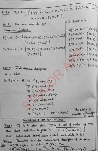
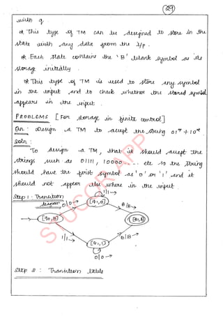
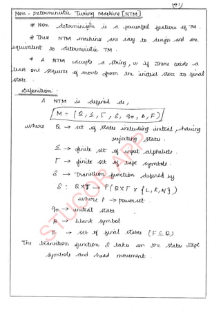
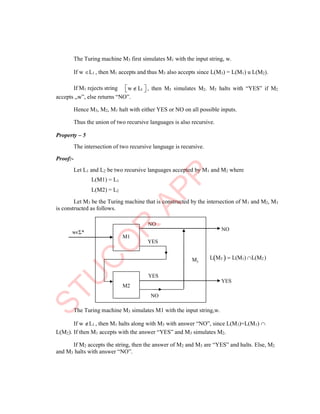
![1.20 Theory of Computation
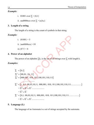
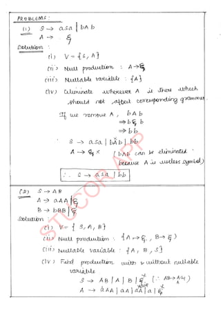
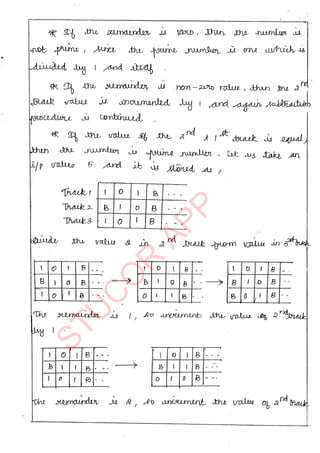
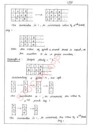
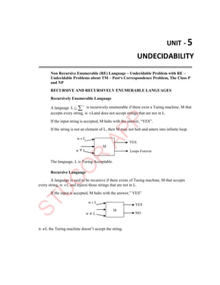
* if we add or subtract 1 from an even integer.
* We get an odd integer
* If we add or subtract 1 from an odd integer we get an even integer.
Basis
For the basis, we choose n = 0. Since there are two statements, each of which must
be proved in both directions (because S1 and S 2 are each “if-and-only-if” statements),
there are actually four cases to the basis, and four cases to the induction as well.
i. [S1; If]
Since 0 is in fact even, we must show that after 0 pushes, the automaton is in state
off. Since that is the start state, the automaton is indeed in state off after 0 pushes.
ii. [S1; Only-if ]
The automaton is in state off after 0 pushes, so we must show that 0 is even. But
0 is even by definition of “even”, so there is nothing more to prove.
iii. [S2; If]
The hypothesis of the “if” part of S2 is that 0 is odd. Since this hypothesis H is
false, any statement of the form “if H then C” is true, which has discussed earlier. Thus,
this part of the basis also holds.
iv. [S2; Only-if]
The hypothesis, that the automaton is in state on after 0 pushes, is also false, since
the only way to get to state on is by following an arc labeled Push, which requires that the
button be pushed at least once. Since the hypothesis is false, we can again conclude that
the if-then statement is true.
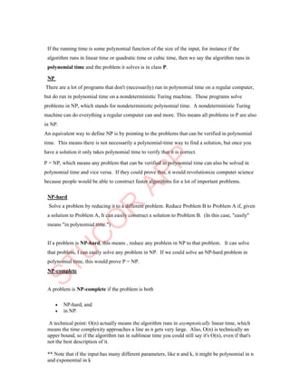
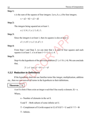
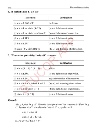
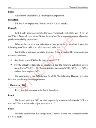
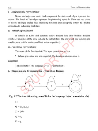
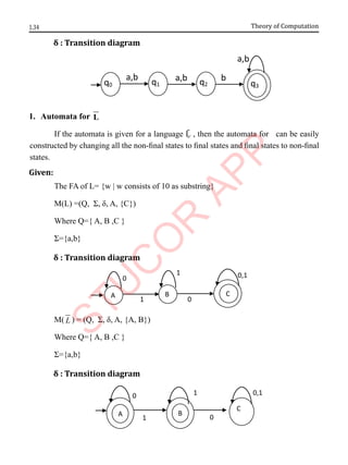
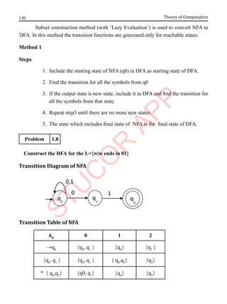
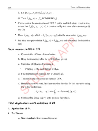
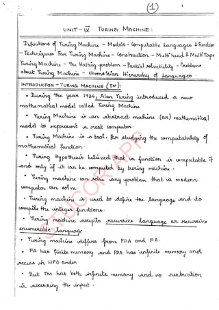
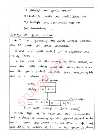
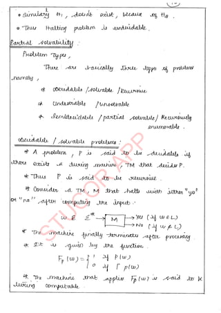
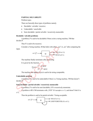
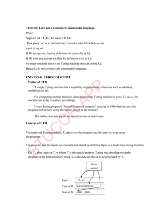
1.5 FInIte AutomAtA
Finite state automaton is an abstract model of a computer. It is represented in the
figure. The components of the automaton are: Input Tape, Finite Control and Tape Head.
Input: String](https://image.slidesharecdn.com/tocnotes-241016035812-7ced6a11/85/theory-of-computation-chapter-2-notes-pdf-20-320.jpg)


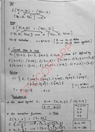
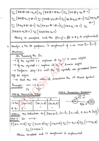
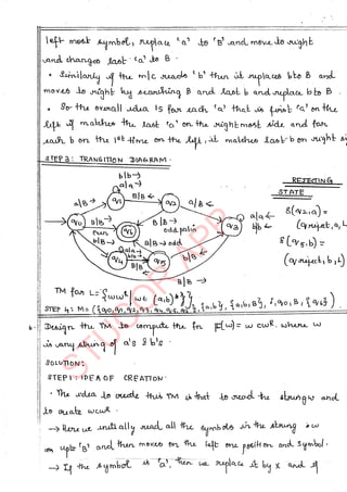
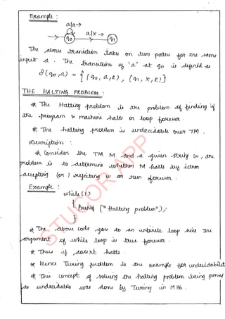
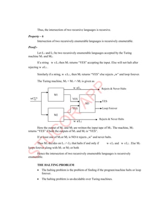
![1.47
Automata Fundamentals
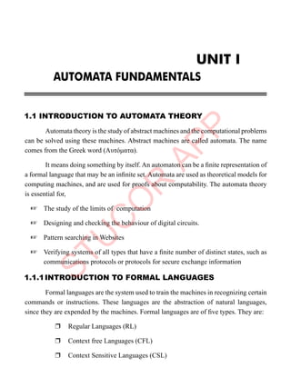
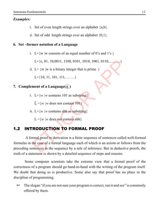
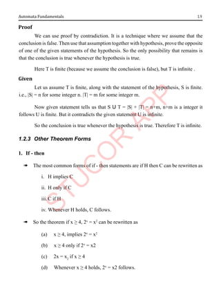
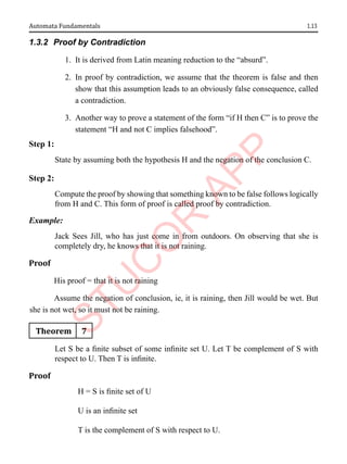
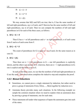
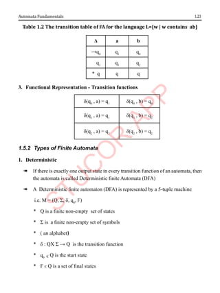
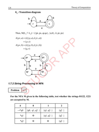
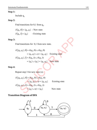
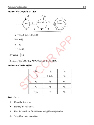
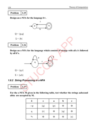
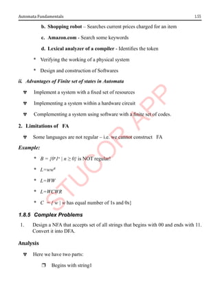
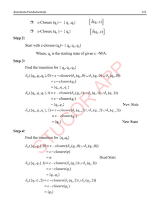
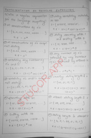
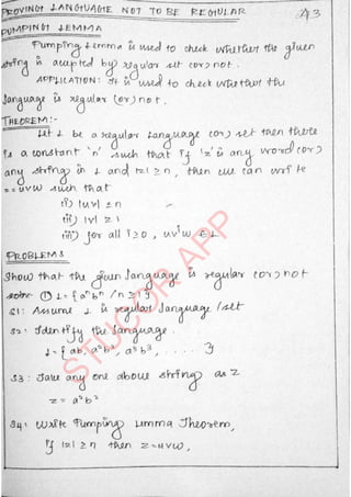
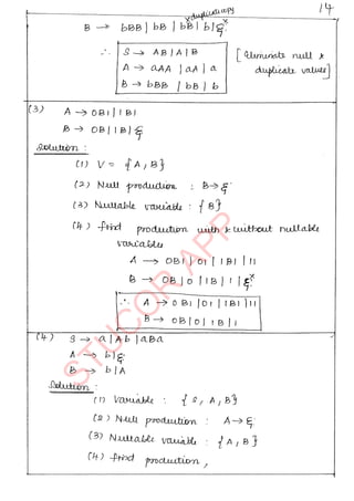
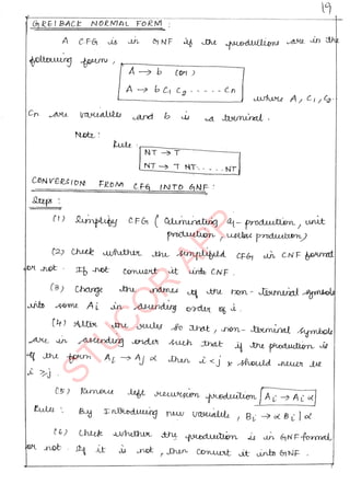
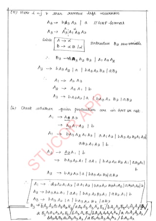
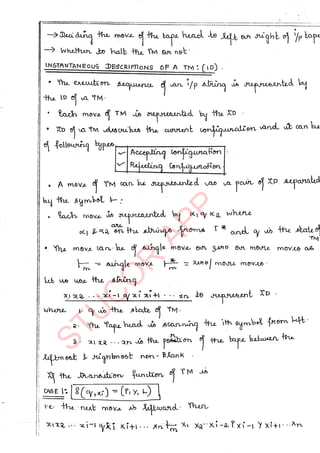
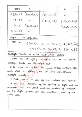
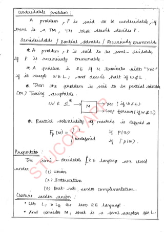
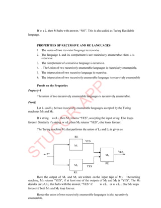
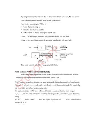
Problem 1.12
Convert to a DFA the following NFA.
0 1
→p {q,s} {q}
*q {r} {q,r}
r {s} {p}
*s - {p}
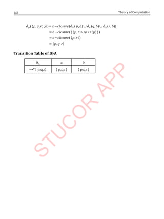
Transition Diagram of DFA
Language of DFA
à The language of a DFA is defined by,
0
ˆ( , )
L(DFA)={w q w is in F}
d
{q,s}
{s}
{r}
[q,
s]
{r,s}
{q,r}
{p,q,r}
{q,r,s}
{p}
1
0
0
1
1
1
1
1 1
0
0
0
0
0
1](https://image.slidesharecdn.com/tocnotes-241016035812-7ced6a11/85/theory-of-computation-chapter-2-notes-pdf-47-320.jpg)
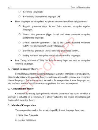
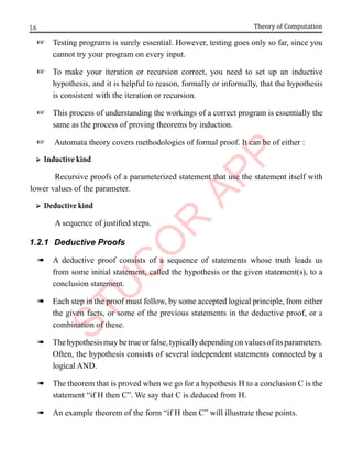
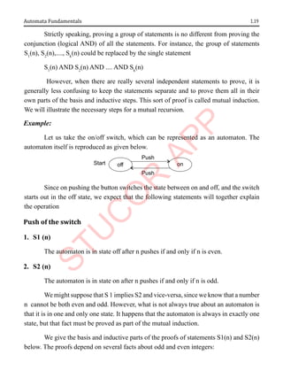
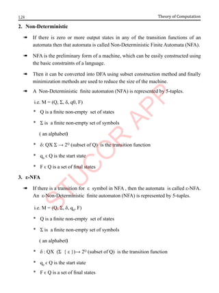
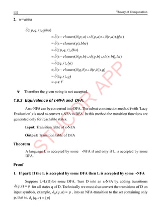
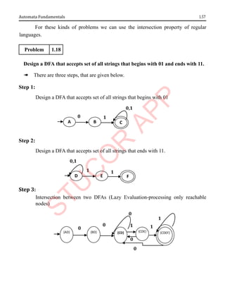
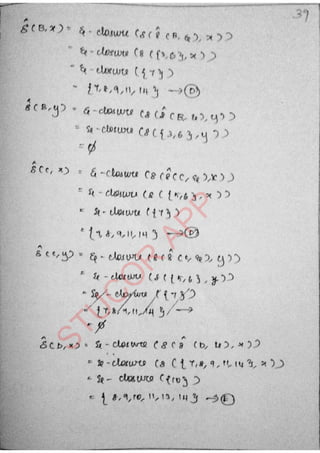
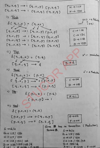
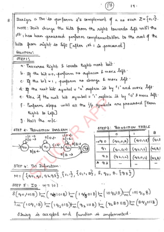
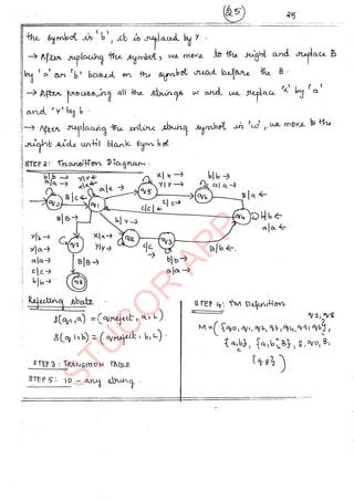
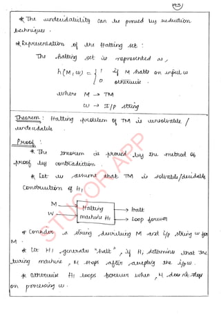
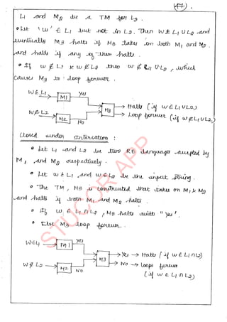
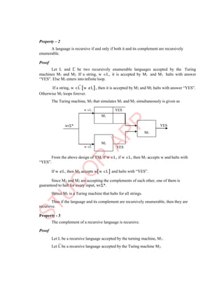
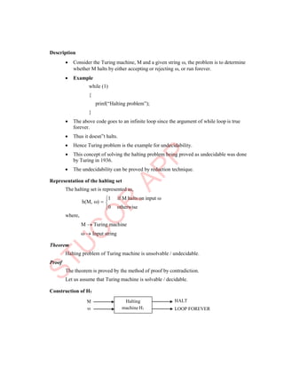
![1.51
Automata Fundamentals
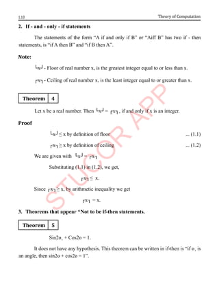
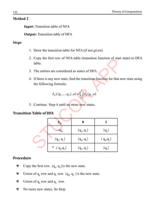
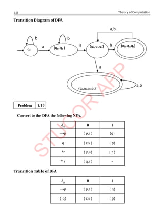
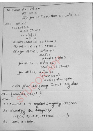
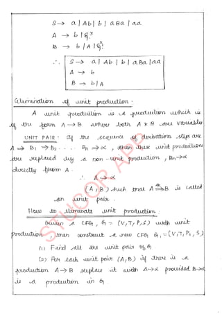
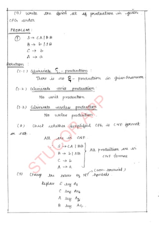
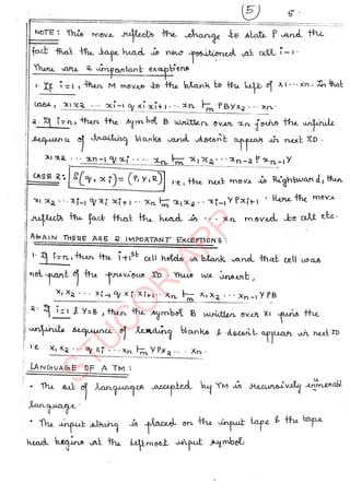
Step 1:
Compute ε-Closure [states that can be reached by traveling along zero or more ε
arrows] for all states .
r ε-Closure (p) = {p,q,r} ˆ( , )
p
d e
r ε-Closure (q) = {q,r}
ˆ( , )
q
d e
r ε-Closure (r ) = {r} ˆ( , )
r
d e
Step2:
Start with ε-closure (p)= {p,q,r}
Where, p is the starting state of given ε –NFA.
1. (p)= {p,q,r}
ˆ({ , , }, )
ˆ( ( ( , ) ( , ) ( , )), )
ˆ( ( ), )
ˆ({ , , }, )
ˆ
p q r aabcc
closure p a q a r a abcc
closure p abcc
p q r abcc
d
d e d d d
d e
d
= − ∪ ∪
= −
=
= ( ( ( , ) ( , ) ( , )), )
ˆ({ , , }, )
ˆ( ( ( , ) ( , ) ( , )), )
ˆ({ , }, )
closure p a q a r a bcc
p q r bcc
closure p b q b r b cc
q r cc
d e d d d
d
d e d d d
d
− ∪ ∪
=
= − ∪ ∪
=
ˆ( ( ( , ) ( , )), )
ˆ({ , }, )
closure q c r c c
q r c
r F
d e d d
d
= − ∪
=
= ∈
^ Therefore the given string is accepted.](https://image.slidesharecdn.com/tocnotes-241016035812-7ced6a11/85/theory-of-computation-chapter-2-notes-pdf-51-320.jpg)
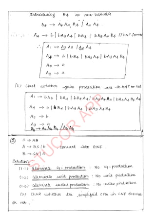
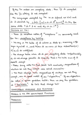
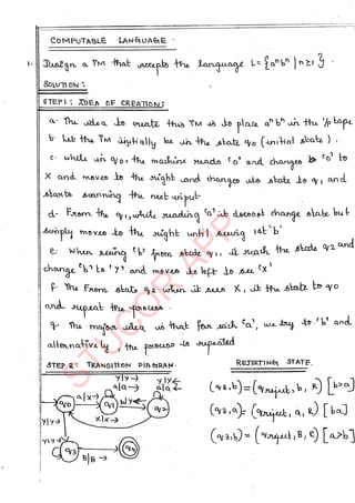
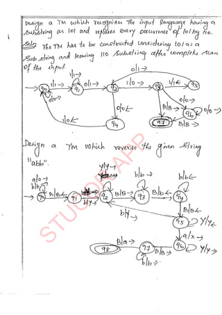
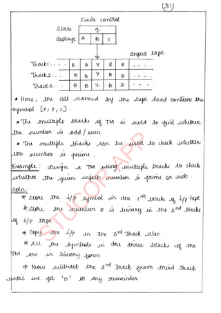
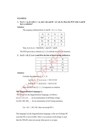
![1.56 Theory of Computation
r Ends with string2
^ Let string1 be considered as s1s2 and string 2 be considered as s3s4 where s1,s2,s3
and s4 are substrings.
^ For all s2 and s3, if s2≠s3, we can easily construct the NFA.
^ In this problem there is no such s2 and s3 where s2=s3. Therefore we can construct
the NFA in one step as follows:
^ The DFA of this machine is given below:
δD
0 1
→ {A} {B} -
{B} {C} -
{C} {C} {C,D}
{C,D} {C} {C,D,E}
* {C,D,E} {C} {C,D,E}
Note: It is difficult to draw the NFA for the following languages wheres2=s3.
^ Set of all strings that begins with 01 and ends with 11 [s2=1]
^ Set of all strings that begins with 01 and ends with 10 [s2=1]
^ Set of all strings that begins with 01 and ends with 01 [s2=01]
^ Set of all strings that begins with 10 and ends with 10 [s2=10]
^ Set of all strings that begins with 00 and ends with 00 [s2=00]
^ Set of all strings that begins with 11 and ends with 11 [s2=00]
1
1
0
0
A B C D E
0,1](https://image.slidesharecdn.com/tocnotes-241016035812-7ced6a11/85/theory-of-computation-chapter-2-notes-pdf-56-320.jpg)
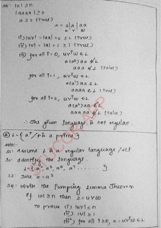
![1.58 Theory of Computation
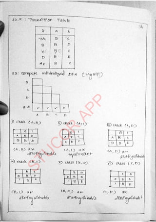
1.8.6 PROBLEMS
1. Consider the following ε-NFA. Covert it into DFA
Transition Table of ε-NFA
δN
ε a b c
→p Ф {p} {q} {r}
q {p} {q} {r} Ф
*r {q} {r} Ф {p}
Step 1:
Compute ε-Closure [states that can be reached by traveling along zero or more ε
arrows] for all states.
r ε-Closure (p) = {p}
ˆ( , )
p
d e
r ε-Closure (q) = {p,q}
ˆ( , )
q
d e
r ε-Closure (r ) = {p,q,r} ˆ( , )
r
d e
Step 2:
Start with ε-closure (p)= {p}
Where, p is the starting state of given ε –NFA.
Step 3:
Find the transition for{p}
({ }, ) ( ( , ))
( )
{ }
({ }, ) ( ( , ))
( )
D N
D N
p a closure p a
closure p
p New State
p b closure p b
closure q
d e d
e
d e d
e
= −
= −
=
= −
= −
{ , }
({ }, ) ( ( , ))
( )
{ , , }
D N
p q New State
p c closure p c
closure r
p q r
d e d
e
=
= −
= −
=](https://image.slidesharecdn.com/tocnotes-241016035812-7ced6a11/85/theory-of-computation-chapter-2-notes-pdf-58-320.jpg)
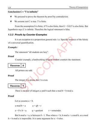
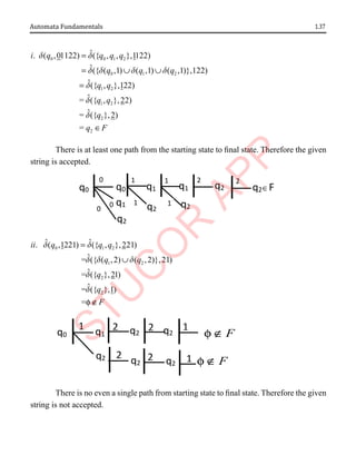
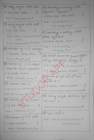
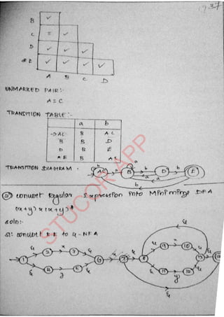
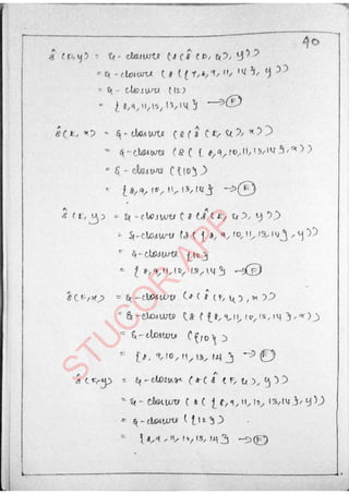
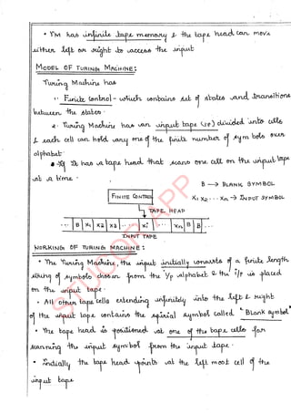
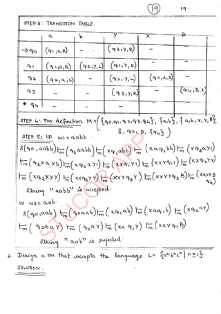
![1.60 Theory of Computation
Transition Diagram of DFA
2. Consider the following ε-NFA. Covert it into DFA
δ ε a b c
→p {q,r} Ф {q} {r}
q Ф {p} {r} {p,q}
*r Ф Ф Ф Ф
Step 1:
Compute ε-Closure [states that can be reached by traveling along zero or more ε
arrows] for all states .
r ε-Closure (p) = {p,q,r}
ˆ( , )
p
d e
r ε-Closure (q) = {q}
ˆ( , )
q
d e
r ε-Closure (r ) = {r}
ˆ( , )
r
d e
Step 2:
Start with ε-closure (p)= {p,q,r}
Where, p is the starting state of given ε - NFA
Step 3:
Find the transition for {p,q,r}
({ , , }, ) ( ( , ) ( , ) ( , ))
( )
{ , , }
D N N N
p q r a closure p a q a r a
closure p
p q r
d e d d d
e
= − ∪ ∪
= −
=
c
b
a a,b,c
b,c
a
{p} {p,q} {p,q,r}](https://image.slidesharecdn.com/tocnotes-241016035812-7ced6a11/85/theory-of-computation-chapter-2-notes-pdf-60-320.jpg)
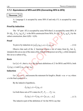
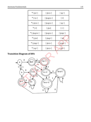
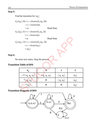
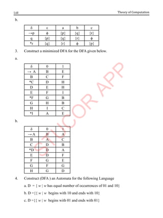
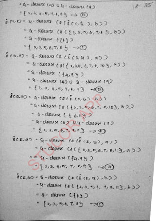
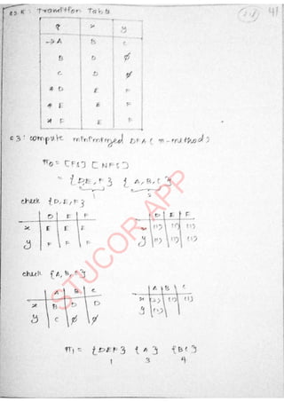
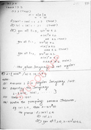
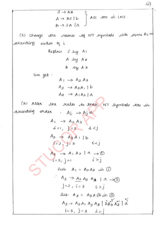
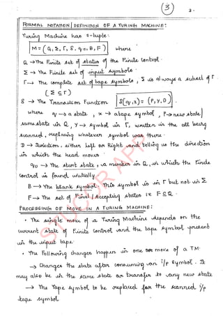
![1.62 Theory of Computation
Step 6:
No more new states. Stop the process.
Transition Table of DFA
δD
a b c
→*{p,q,r} {p,q,r} {q,r} {p,q,r}
*{q,r} {p,q,r} {r} {p,q,r}
*{r} Ф Ф Ф
Transition Diagram of DFA
3. Consider the following ε-NFA. Covert a,b,c it into DFA.
Transition Table of ε-NFA
δN
ε 0 1 2
→ q0
q1
q0
Ф Ф
q1
q2
Ф q1
Ф
*q2
Ф Ф Ф q2
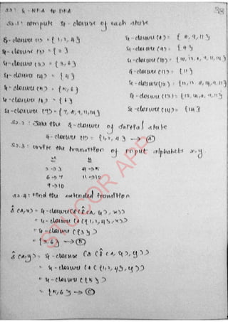
Step 1:
Compute ε-Closure [states that can be reached by traveling along zero or more ε
arrows] for all states .
r ε-Closure (q0
) = { q0
, q1
, q2
} 0
ˆ( , )
q
d e
b
b
a,c
{q,r} {r}
Ф
{p,q,r}
a,c](https://image.slidesharecdn.com/tocnotes-241016035812-7ced6a11/85/theory-of-computation-chapter-2-notes-pdf-62-320.jpg)
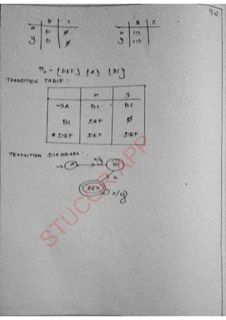
![1.65
Automata Fundamentals
Q = {{q0
, q1
, q2
},{ q1
, q2
},{q2
} }
Σ = {0,1,2}
q0
= {q0
, q1
, q2
}
F = {{q0
, q1
, q2
},{ q1
, q2
},{q2
}}
4. Consider the following ε-NFA. Covert it into DFA
δN
ε a b
→ p {r} {q} {p,r}
q Ф {p} Ф
*r {p,q} {r} {p}
Step 1:
Compute ε-Closure [states that can be reached by traveling along zero or more ε
arrows] for all states.
r ε-Closure (p) = {p,q,r}
ˆ( , )
p
d e
r ε-Closure (q) = {q}
ˆ( , )
q
d e
r ε-Closure (r ) = {p,q,r} ˆ( , )
r
d e
Step 2:
Start with ε-closure (p)= { p, q, r}
Where, p is the starting state of given ε –NFA
Step 3:
Find the transition for { p,q,r}
({ , , }, ) ( ( , ) ( , ) ( , ))
( )
( , , )
{ , , }
D N N N
p q r a closure p a q a r a
closure q p r
closure p q r
p q r
d e d d d
e
e
= − ∪ ∪
= − ∪ ∪
= −
=](https://image.slidesharecdn.com/tocnotes-241016035812-7ced6a11/85/theory-of-computation-chapter-2-notes-pdf-65-320.jpg)


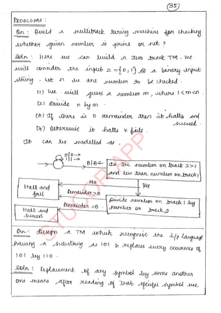

![
p
Partial solvability of a machine is defined as,
F ()
1 if p()
undefined if p()
Enumerating a language
Consider a k-tape turing machine. Then the machine M enumerates the language L
(such that L ∑*) if
The tape head never moves to the left on the first tape.
No blank symbol (B) on the first tape is erased or modified.
For all L, where there exists a transition rule, i on tape 1 with contents
1 # 2 # 3 # ... # n # # (for n 0)
Where 1, 2 , 3, ....., n , are distinct elements on L.
If L is finite, then nothing is printed after the # of the left symbol
That is,
If L is a finite language then the TM, M either
o Halts normally after all the elements appear on the first tape (elements are
processed)
or
o Continue to process and make moves and state changes without
scanning/printing other string on the first tape.
If the language, L is finite, the Turing machine runs forever.
Theorem
A language L ∑* is recursively enumerable if and only if L can be enumerated by
some TM.
Proof
k(M1)].
Let M1 be a Turing machine that enumerates L.
And let M2 accepts L. M2 can be constructed as a k-tape Turing machine [k(M2) >
M2 simulates M1 and M1 pauses whenever M2 scans the „#‟ symbol.](https://image.slidesharecdn.com/tocnotes-241016035812-7ced6a11/85/theory-of-computation-chapter-2-notes-pdf-300-320.jpg)
![d
Depending on om [m=1 stop, m=2 Left, m=3Right], move the head on
tape-2 to the position of the next 1 to the left/right/stop accordingly
If TM has no transition, matching the simulated state and tape symbol, then no
transition will be found. This happens when the TM stops also.
If the TM, T enters halt (accepting state), then UTM accepts the input, w
Thus for every coded pair <T, w>, UTM simulates T on w, if and only if T accepts the
input string, w.
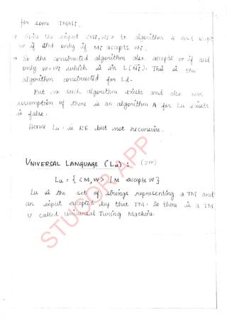
Thus U TM simulates M and accepts W.Thus Lu is recursively enumerable
Definition of Universal Language [Lu]
The universal language, Lu is the set of all binary strings , where represents the
ordered pair <T, w> where
T Turing machine
w any input string accepted by T
It can also be represented as = e(T) e(w) .
Theorem
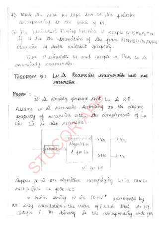
Lu is the recursively enumerable but not recursive .
Proof
From the definition and operations of UTM, we know that Lu is recursively
enumerable.
Lu accepts the string w if it is processed by the TM,T. Else, rejects „w‟ and the
machine doesn‟t halts forever.
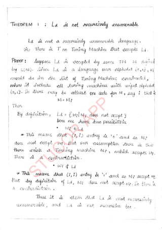
To prove that Lu is not recursive, the proof can be done by contradiction. Let Lu is
Turing decidable [recursive], and then by definitionacceptable.
Lu (complement of Lu) is Turing
We can show that Lu is Turing acceptable, that leads to Ld to be Turing acceptable.
But we know that Ld is not Turing acceptable.
Hence Lu is not Turing decidable by proof by contradiction.
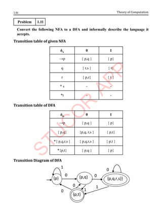
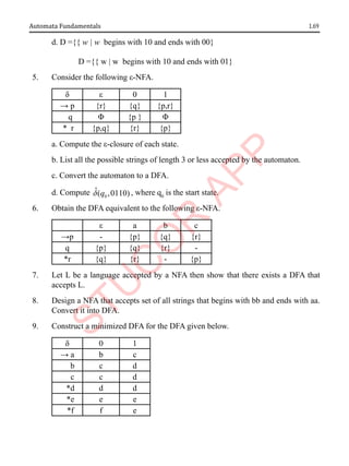
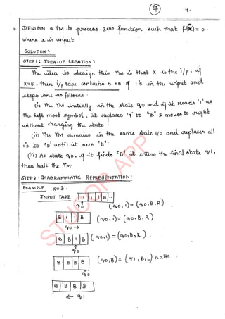
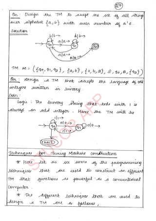
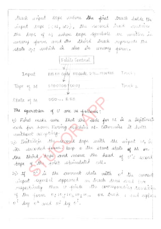
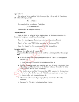
Proof on Lu is during acceptable Ld is Turing acceptable
w
Suppose “A” is the algorithm that recognizes Lu .
Then L is recognizes as follows. Given a string w(0,1)*
determined easily, the
value of I such that w = wi.
Integer value, I in binary is the corresponding code for TM, Ti. Provide <Ti, wi> to the
Accept Accept
w111w
Reject Reject
T for Ld
Copy
Hypothetical
algorithm
T for Lu](https://image.slidesharecdn.com/tocnotes-241016035812-7ced6a11/85/theory-of-computation-chapter-2-notes-pdf-305-320.jpg)