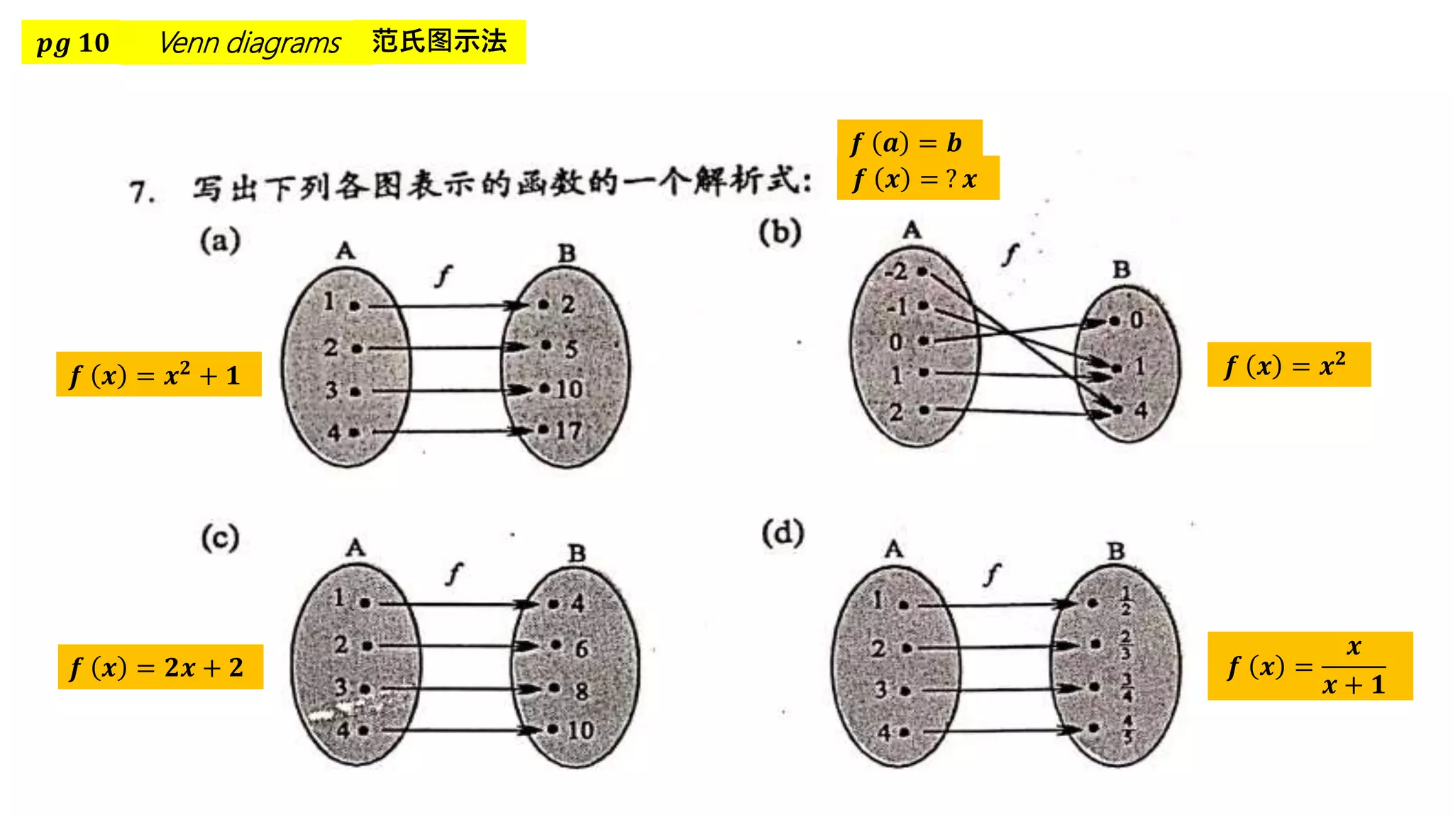
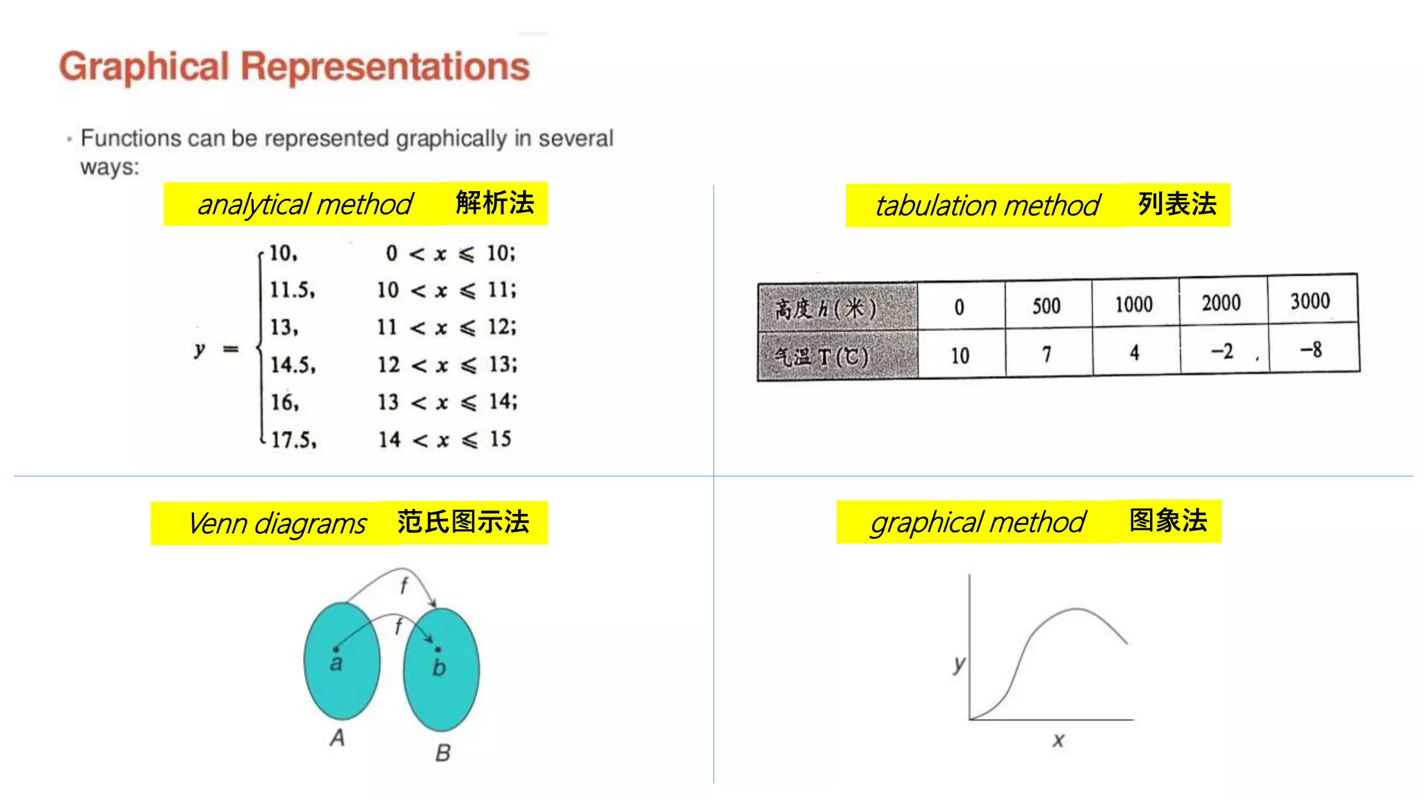
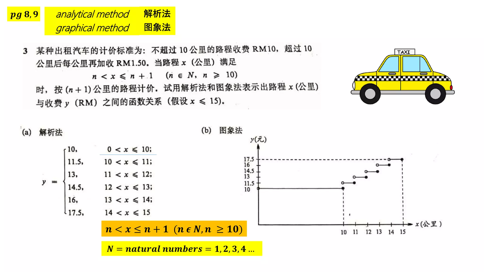
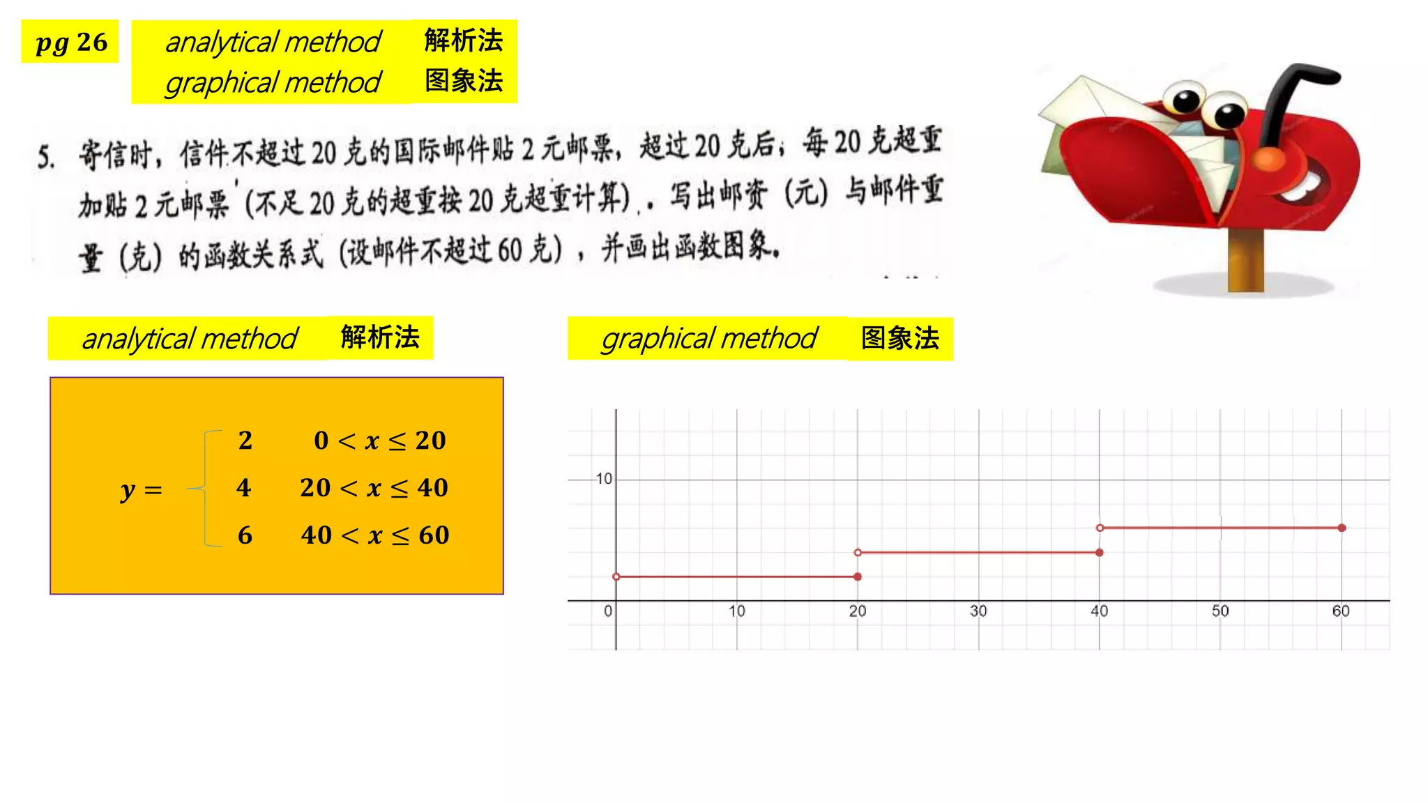
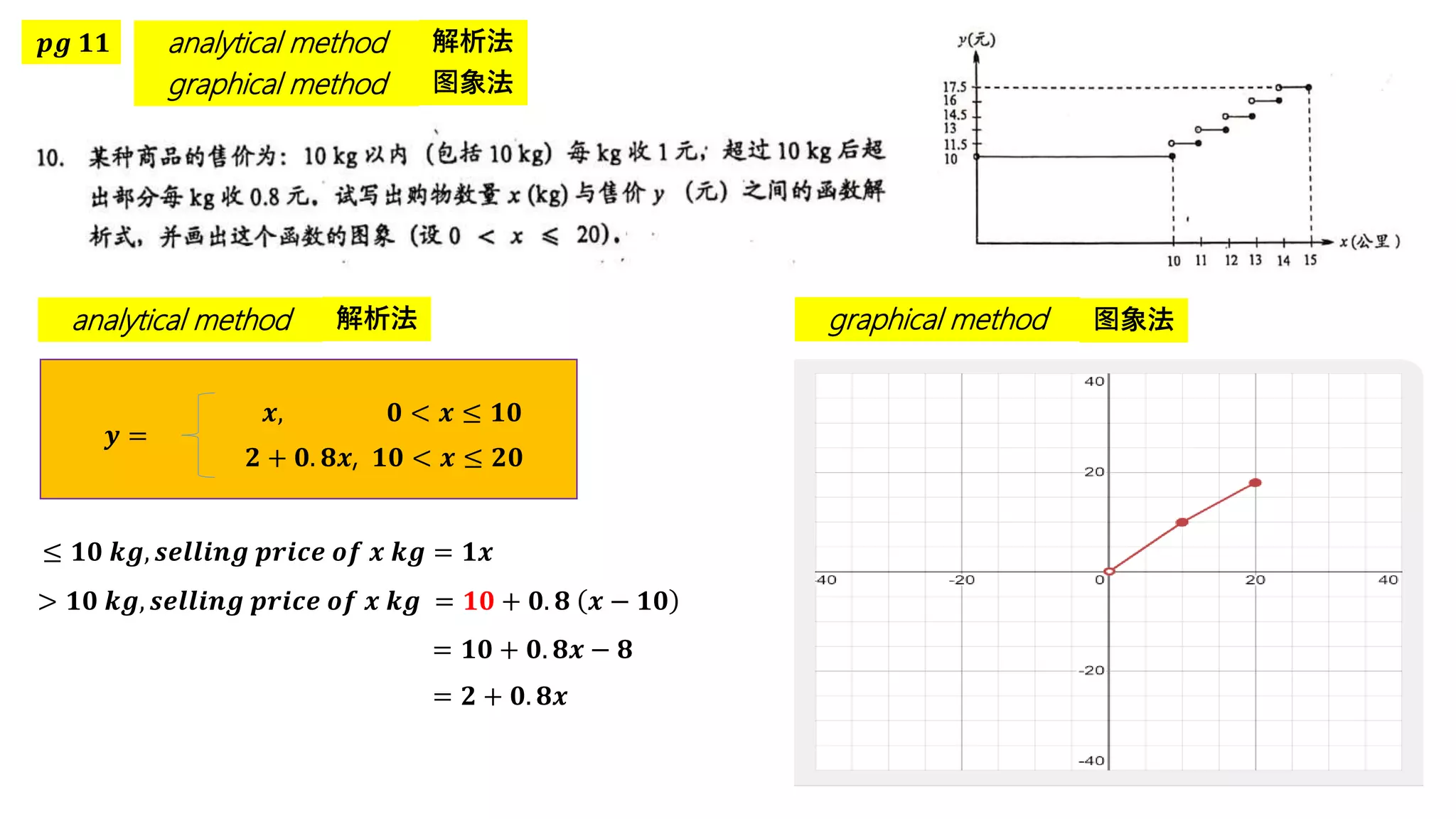
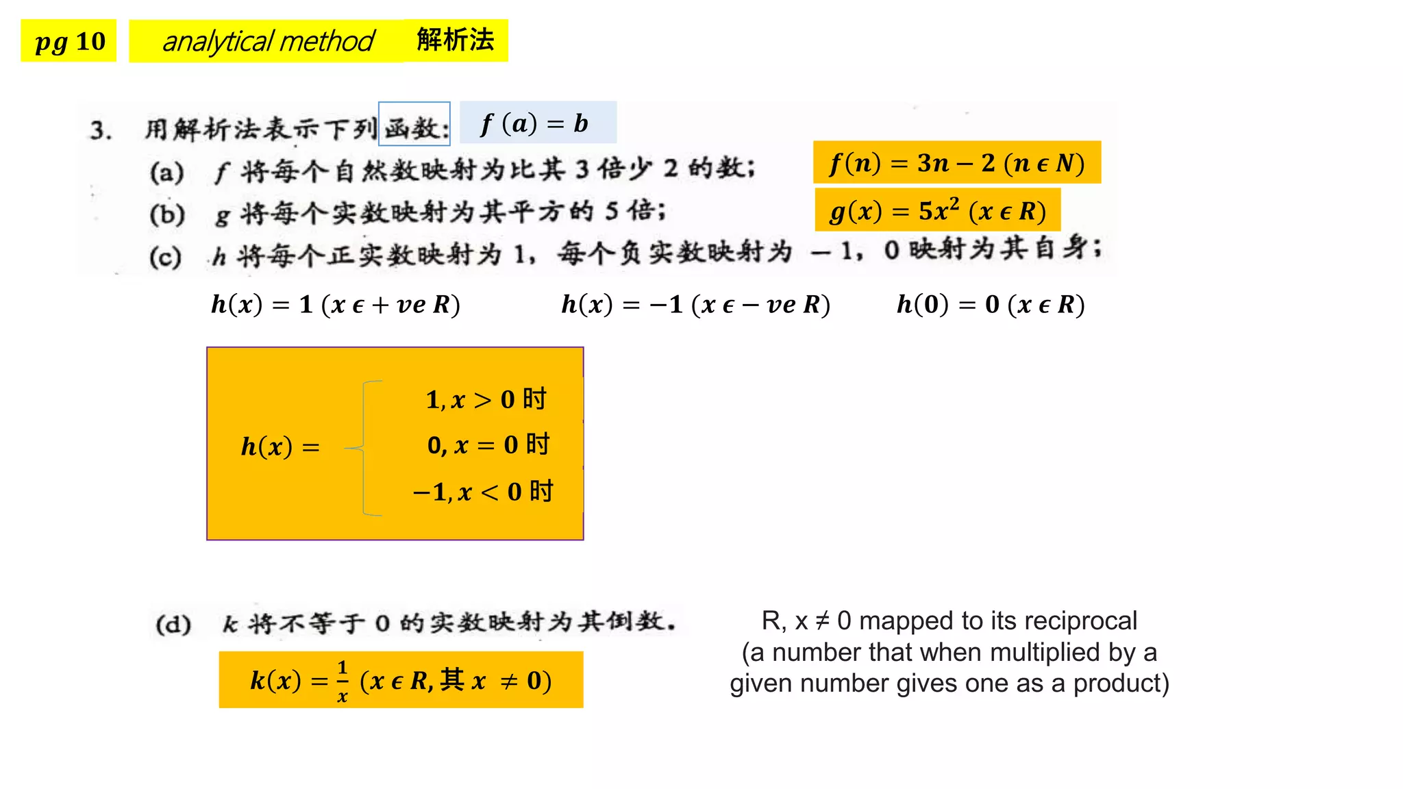
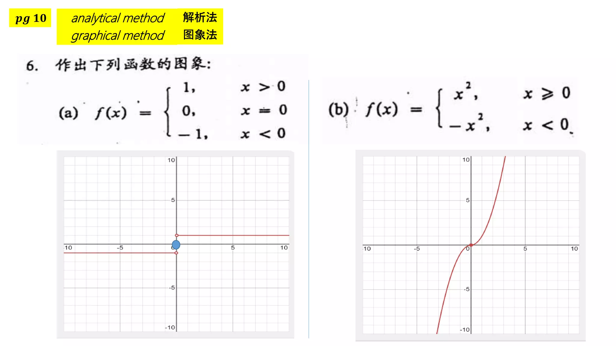
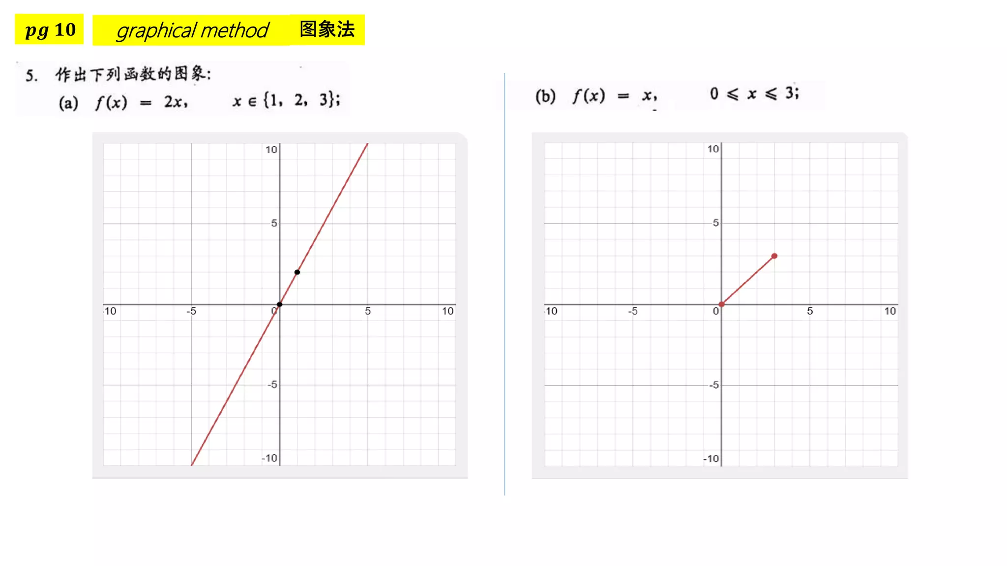
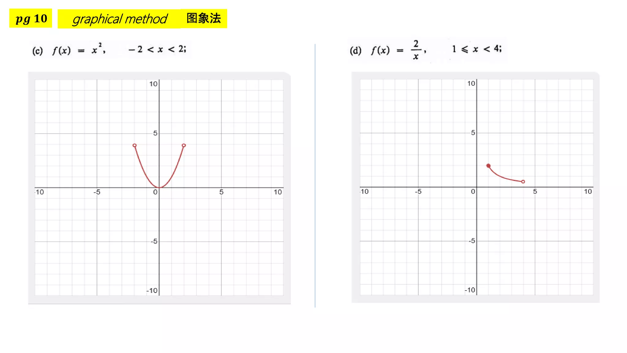
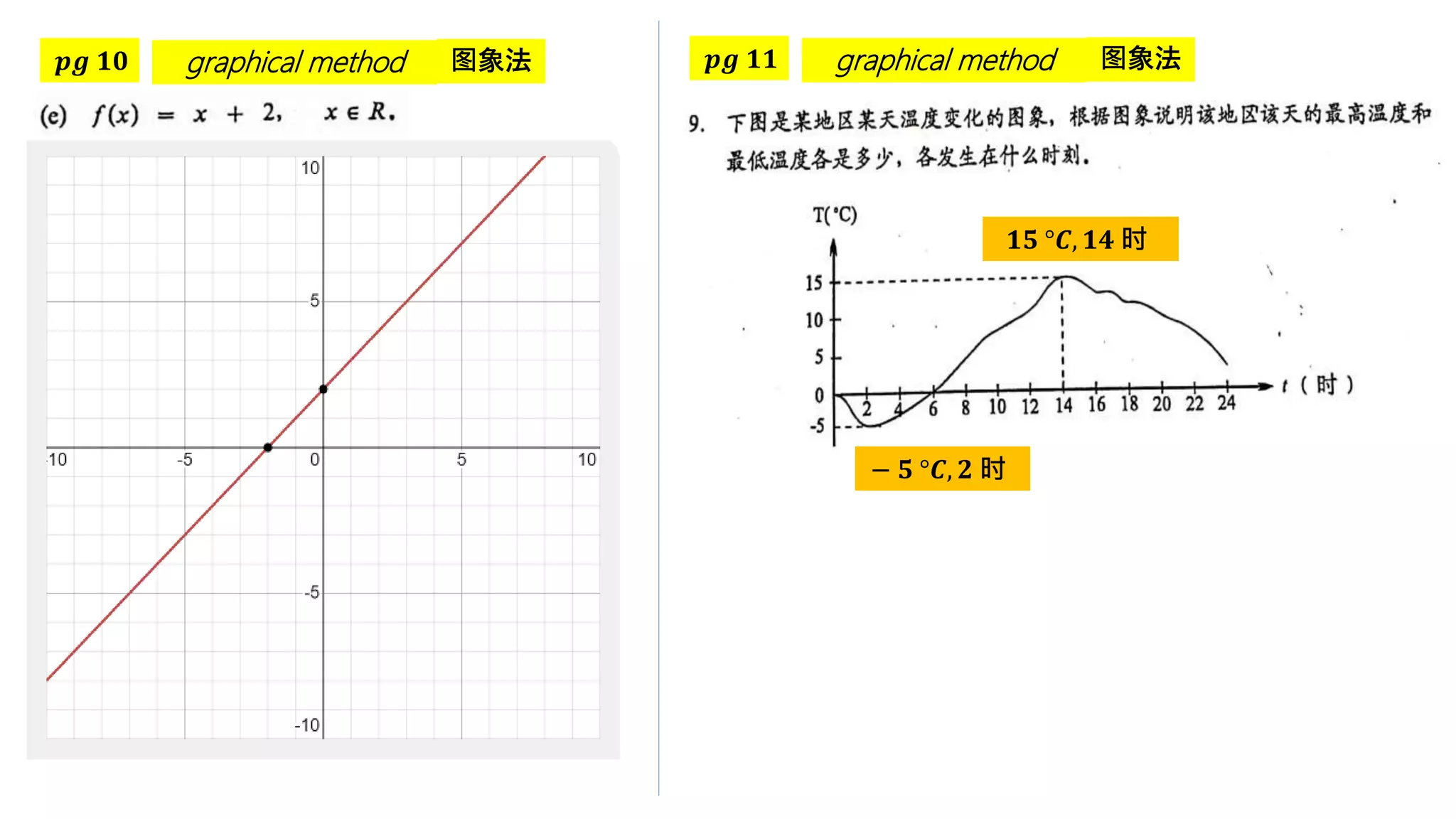
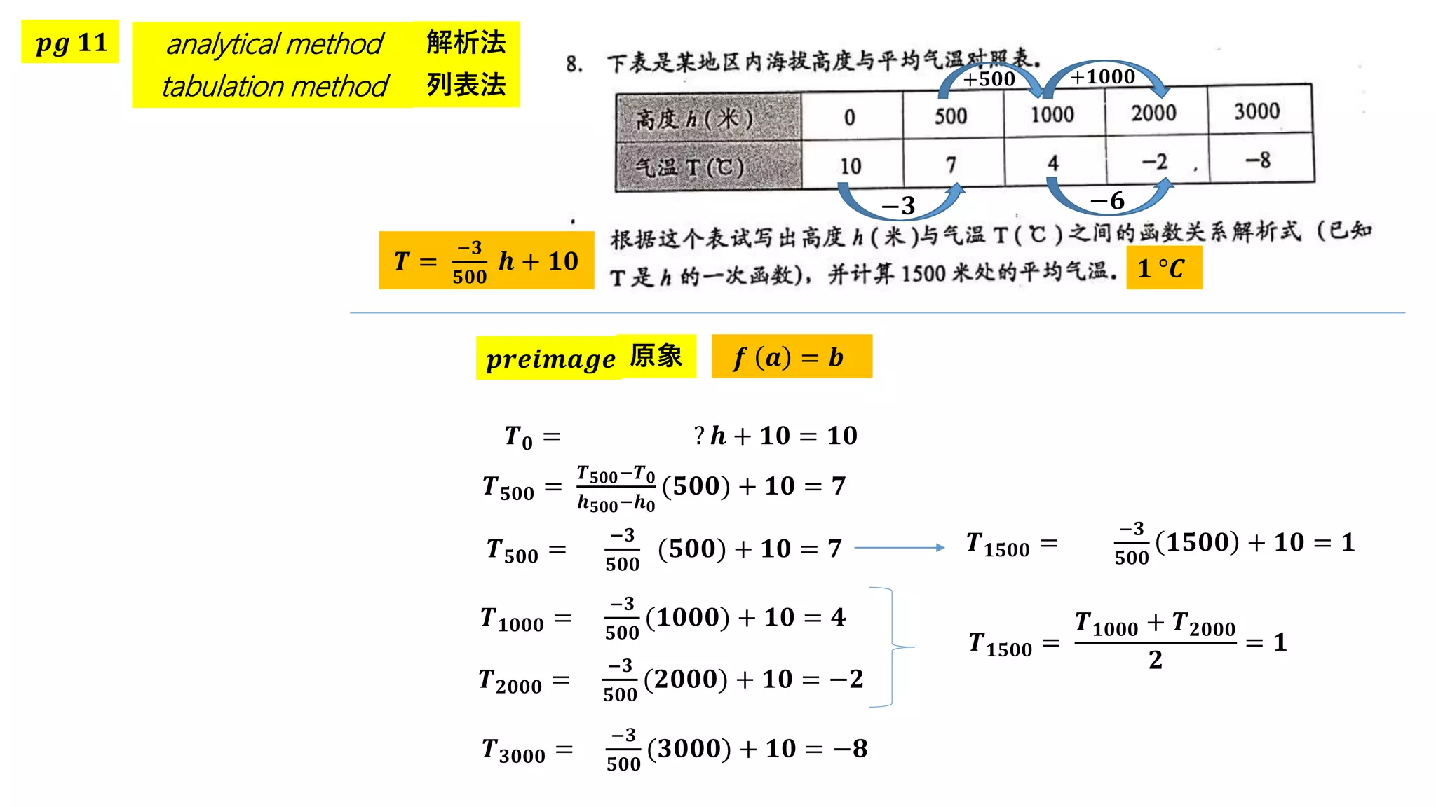
This document provides an overview of MATLAB and image processing. It discusses basic MATLAB commands and functions like arithmetic operations, if/else statements, for/while loops, functions, plotting and graphing, loading and saving data, multidimensional arrays, and effective MATLAB coding techniques like vectorization. The document also mentions commands for plotting, legend, axis, loading and saving data, and reserving memory space using zeros.
Grade 10_Math-Lesson 2-3 Graphs of Polynomial Functions .pptxErlenaMirador1
The document discusses how to graph polynomial functions by determining:
1) The end behavior using the leading coefficient test
2) The maximum number of turning points from the degree of the polynomial
3) The x-intercepts by finding the zeros of the polynomial
4) The y-intercept by evaluating the polynomial at x=0
It provides examples of using these steps to graph various polynomial functions of degrees 1-5.
SUEC 高中 Adv Maths (Quadratic Equation in One Variable)tungwc
Sources:
Visual - various maths sites (credits to original creator)
Questions - Dong Zong's Textbook
suitable for SUEC (Maths), SPM (Maths and Add Maths) too
This document discusses regression lines and linear regression. It defines independent and dependent variables in scatter plots. The best-fit line, or line of best fit, is the straight line that best illustrates the trend of data points in a scatter plot. The regression equation for a best-fit line is y=mx + b, where m is the slope and b is the y-intercept. Formulas are provided to calculate the slope and y-intercept from sample data. Two examples are worked through to find the regression equation for sets of (x, y) data points and estimate y values.
References:
"Gaussian Process", Lectured by Professor Il-Chul Moon
"Gaussian Processes", Cornell CS4780 , Lectured by Professor
Kilian Weinberger
Bayesian Deep Learning by Sungjoon Choi
Sources:
Visual - various maths sites (credits to original creator)
Questions - Dong Zong's Textbook
suitable for SUEC (Maths), SPM (Maths and Add Maths) too
Here are the steps to solve the quadratic equations given in the seatwork:
1) x2 = 64
Take the square root of both sides:
x = ±8
2) 3x2 = 108
Take the square root of both sides:
x = ±6
3) x2 - 6 = 0
Factor: (x + 3)(x - 2) = 0
x = -3, 2
4) x2 - 21 = 0
Take the square root of both sides:
x = ±√21
5) m2 + 16m = 4
Complete the square: (m + 8)2 = 16
Take the square root of both sides:
Differential Geometry for Machine LearningSEMINARGROOT
References:
Differential Geometry of Curves and Surfaces, Manfredo P. Do Carmo (2016)
Differential Geometry by Claudio Arezzo
Youtube: https://youtu.be/tKnBj7B2PSg
What is a Manifold?
Youtube: https://youtu.be/CEXSSz0gZI4
Shape analysis (MIT spring 2019) by Justin Solomon
Youtube: https://youtu.be/GEljqHZb30c
Tensor Calculus
Youtube: https://youtu.be/kGXr1SF3WmA
Manifolds: A Gentle Introduction,
Hyperbolic Geometry and Poincaré Embeddings by Brian Keng
Link: http://bjlkeng.github.io/posts/manifolds/,
http://bjlkeng.github.io/posts/hyperbolic-geometry-and-poincare-embeddings/
Statistical Learning models for Manifold-Valued measurements with application to computer vision and neuroimaging by Hyunwoo J.Kim
- A rational expression is a ratio of two polynomial expressions, where the denominator is not equal to zero.
- To find the domain of a rational expression, set the denominator equal to zero and solve for values of x that make the denominator equal to zero. These values are excluded from the domain.
- To find the range, find the horizontal asymptote by comparing the degrees of the numerator and denominator. The range is all real numbers except the constant value of the horizontal asymptote.
The document presents an approach for intensity constrained gradient-based image reconstruction. It aims to find an image I(x) that minimizes an energy function involving both the intensity difference between the image and a given intensity map, and the gradient difference between the image and a given gradient map. This is formulated as an Euler-Lagrange differential equation, which is then discretized and solved using the discrete cosine transform to obtain the reconstructed image. Code for implementing this approach is available online, and references are provided for related work.
Main obstacles of Bayesian statistics or Bayesian machine learning is computing posterior distribution. In many contexts, computing posterior distribution is intractable. Today, there are two main stream to detour directly computing posterior distribution. One is using sampling method(ex. MCMC) and another is Variational inference. Compared to Variational inference, MCMC takes more time and vulnerable to high-dimensional parameters. However, MCMC has strength in simplicity and guarantees of convergence. I'll briefly introduce several methods people using in application.
Generalised Statistical Convergence For Double SequencesIOSR Journals
Recently, the concept of 𝛽-statistical Convergence was introduced considering a sequence of infinite
matrices 𝛽 = (𝑏𝑛𝑘 𝑖 ). Later, it was used to define and study 𝛽-statistical limit point, 𝛽-statistical cluster point,
𝑠𝑡𝛽 − 𝑙𝑖𝑚𝑖𝑡 inferior and 𝑠𝑡𝛽 − 𝑙𝑖𝑚𝑖𝑡 superior. In this paper we analogously define and study 2𝛽-statistical
limit, 2𝛽-statistical cluster point, 𝑠𝑡2𝛽 − 𝑙𝑖𝑚𝑖𝑡 inferior and 𝑠𝑡2𝛽 − 𝑙𝑖𝑚𝑖𝑡 superior for double sequences.
This document discusses graph colouring and graph dynamical systems. It begins with an overview of graph theory concepts like graphs, graph colouring, and the graph colouring problem. It then discusses deterministic finite automata and introduces graph-cellular automata as a type of graph dynamical system. Specific examples of graph-cellular automata on linear graphs, circle graphs, tree graphs, wheel graphs, and Peterson graphs are analyzed. The results show that linear graphs, circle graphs, and tree graphs reach a stable coloring, while wheel graphs and Peterson graphs result in a loop.
1. The document provides analytical solutions and MATLAB code for various types of differential equations, including separable, homogeneous, exact, and linear differential equations.
2. Applications include models for thermometer cooling, concentration of dye in a mixing tank, and hydrodynamic experiments in a tank.
3. Methods demonstrated include finding integrating factors by inspection or determining integrating factors when a differential equation is not exact.
The EM algorithm is an iterative method to find maximum likelihood estimates of parameters in probabilistic models with latent variables. It has two steps: E-step, where expectations of the latent variables are computed based on current estimates, and M-step, where parameters are re-estimated to maximize the expected complete-data log-likelihood found in the E-step. As an example, the EM algorithm is applied to estimate the parameters of a Gaussian mixture model, where the latent variables indicate component membership of each data point.
The document discusses applications of vector spaces and subspaces in telecommunications engineering. It provides examples of how vector spaces are used in areas like electromagnetic wave transmission, wired and wireless data transmission, and color image coding. Vector spaces allow modeling of physical phenomena like electric and magnetic field vectors. Color spaces also represent vector spaces used in television systems. Matrix transformations are used to relate different color spaces like RGB and YCbCr. The document concludes that linear algebra provides engineers powerful mathematical tools for solving problems across telecommunications.
Mpc 006 - 02-03 partial and multiple correlationVasant Kothari
3.2 Partial Correlation (rp)
3.2.1 Formula and Example
3.2.2 Alternative Use of Partial Correlation
3.3 Linear Regression
3.4 Part Correlation (Semipartial correlation) rsp
3.4.1 Semipartial Correlation: Alternative Understanding
3.5 Multiple Correlation Coefficient (R)
The document discusses systems of two variable equations and inequalities. It defines a system of two variable equations as a collection of two or more equations involving two variables (linear-linear, linear-quadratic, quadratic-quadratic) whose solutions are points satisfying the equations. The solution graph is the intersection of the equations. It also defines systems of two variable inequalities and explains how to graphically represent the solution sets. Examples of solving systems using graphical and substitution methods are provided.
PR 113: The Perception Distortion TradeoffTaeoh Kim
The document discusses the perception-distortion tradeoff in image processing tasks. It presents three key points:
1) Algorithms cannot simultaneously achieve low distortion (error) and good perceptual quality when processing images. There is a inherent tradeoff between these two goals.
2) Distortion measures how similar the processed image is to the ground truth, while perceptual quality measures how natural the processed image looks.
3) The perception-distortion function is proven to be monotonically non-increasing and convex, meaning small gains in one area (distortion or perception) require large losses in the other.
Intro to Quant Trading Strategies (Lecture 2 of 10)Adrian Aley
This document provides an introduction to hidden Markov models for algorithmic trading strategies. It discusses key concepts like Bayes' theorem, Markov chains, and the Markov property. It then covers the three main problems in hidden Markov models: likelihood, decoding, and learning. It presents solutions to these problems, including the forward-backward, Viterbi, and Baum-Welch algorithms. It also discusses extensions to non-discrete distributions and trading ideas using hidden Markov models.
"Incremental Lossless Graph Summarization", KDD 2020지훈 고
A presentation slides of Jihoon Ko*, Yunbum Kook* and Kijung Shin, "Incremental Lossless Graph Summarization", KDD 2020.
Given a fully dynamic graph, represented as a stream of edge insertions and deletions, how can we obtain and incrementally update a lossless summary of its current snapshot?
As large-scale graphs are prevalent, concisely representing them is inevitable for efficient storage and analysis. Lossless graph summarization is an effective graph-compression technique with many desirable properties. It aims to compactly represent the input graph as (a) a summary graph consisting of supernodes (i.e., sets of nodes) and superedges (i.e., edges between supernodes), which provide a rough description, and (b) edge corrections which fix errors induced by the rough description. While a number of batch algorithms, suited for static graphs, have been developed for rapid and compact graph summarization, they are highly inefficient in terms of time and space for dynamic graphs, which are common in practice.
In this work, we propose MoSSo, the first incremental algorithm for lossless summarization of fully dynamic graphs. In response to each change in the input graph, MoSSo updates the output representation by repeatedly moving nodes among supernodes. MoSSo decides nodes to be moved and their destinations carefully but rapidly based on several novel ideas. Through extensive experiments on 10 real graphs, we show MoSSo is (a) Fast and 'any time': processing each change in near-constant time (less than 0.1 millisecond), up to 7 orders of magnitude faster than running state-of-the-art batch methods, (b) Scalable: summarizing graphs with hundreds of millions of edges, requiring sub-linear memory during the process, and (c) Effective: achieving comparable compression ratios even to state-of-the-art batch methods.
The document provides an introduction to variational autoencoders (VAE). It discusses how VAEs can be used to learn the underlying distribution of data by introducing a latent variable z that follows a prior distribution like a standard normal. The document outlines two approaches - explicitly modeling the data distribution p(x), or using the latent variable z. It suggests using z and assuming the conditional distribution p(x|z) is a Gaussian with mean determined by a neural network gθ(z). The goal is to maximize the likelihood of the dataset by optimizing the evidence lower bound objective.
SPM BM K1 Bahagian A (Contoh Surat Aduan).pptxtungwc
Penduduk Taman Cengal membuat aduan tentang masalah kutipan sampah yang tidak berjadual dan tidak sempurna, menyebabkan timbunan sampah dan bau. Mereka meminta pihak berkuasa tempatan menguruskan kutipan sampah secara berjadual dan memberi maklum balas.
The document discusses random phenomena and probability. It defines a random phenomenon as one where individual outcomes are uncertain. It provides examples of sample spaces and sample points for events like goals in a game or coin flips. It also includes examples of calculating probabilities of certain outcomes occurring based on the sample space and equally likely outcomes, such as the probability of getting 3 heads in a row or having at least 1 head.
More Related Content
Similar to SUEC 高中 Adv Maths (Function Graphical Representation)
Here are the steps to solve the quadratic equations given in the seatwork:
1) x2 = 64
Take the square root of both sides:
x = ±8
2) 3x2 = 108
Take the square root of both sides:
x = ±6
3) x2 - 6 = 0
Factor: (x + 3)(x - 2) = 0
x = -3, 2
4) x2 - 21 = 0
Take the square root of both sides:
x = ±√21
5) m2 + 16m = 4
Complete the square: (m + 8)2 = 16
Take the square root of both sides:
Differential Geometry for Machine LearningSEMINARGROOT
References:
Differential Geometry of Curves and Surfaces, Manfredo P. Do Carmo (2016)
Differential Geometry by Claudio Arezzo
Youtube: https://youtu.be/tKnBj7B2PSg
What is a Manifold?
Youtube: https://youtu.be/CEXSSz0gZI4
Shape analysis (MIT spring 2019) by Justin Solomon
Youtube: https://youtu.be/GEljqHZb30c
Tensor Calculus
Youtube: https://youtu.be/kGXr1SF3WmA
Manifolds: A Gentle Introduction,
Hyperbolic Geometry and Poincaré Embeddings by Brian Keng
Link: http://bjlkeng.github.io/posts/manifolds/,
http://bjlkeng.github.io/posts/hyperbolic-geometry-and-poincare-embeddings/
Statistical Learning models for Manifold-Valued measurements with application to computer vision and neuroimaging by Hyunwoo J.Kim
- A rational expression is a ratio of two polynomial expressions, where the denominator is not equal to zero.
- To find the domain of a rational expression, set the denominator equal to zero and solve for values of x that make the denominator equal to zero. These values are excluded from the domain.
- To find the range, find the horizontal asymptote by comparing the degrees of the numerator and denominator. The range is all real numbers except the constant value of the horizontal asymptote.
The document presents an approach for intensity constrained gradient-based image reconstruction. It aims to find an image I(x) that minimizes an energy function involving both the intensity difference between the image and a given intensity map, and the gradient difference between the image and a given gradient map. This is formulated as an Euler-Lagrange differential equation, which is then discretized and solved using the discrete cosine transform to obtain the reconstructed image. Code for implementing this approach is available online, and references are provided for related work.
Main obstacles of Bayesian statistics or Bayesian machine learning is computing posterior distribution. In many contexts, computing posterior distribution is intractable. Today, there are two main stream to detour directly computing posterior distribution. One is using sampling method(ex. MCMC) and another is Variational inference. Compared to Variational inference, MCMC takes more time and vulnerable to high-dimensional parameters. However, MCMC has strength in simplicity and guarantees of convergence. I'll briefly introduce several methods people using in application.
Generalised Statistical Convergence For Double SequencesIOSR Journals
Recently, the concept of 𝛽-statistical Convergence was introduced considering a sequence of infinite
matrices 𝛽 = (𝑏𝑛𝑘 𝑖 ). Later, it was used to define and study 𝛽-statistical limit point, 𝛽-statistical cluster point,
𝑠𝑡𝛽 − 𝑙𝑖𝑚𝑖𝑡 inferior and 𝑠𝑡𝛽 − 𝑙𝑖𝑚𝑖𝑡 superior. In this paper we analogously define and study 2𝛽-statistical
limit, 2𝛽-statistical cluster point, 𝑠𝑡2𝛽 − 𝑙𝑖𝑚𝑖𝑡 inferior and 𝑠𝑡2𝛽 − 𝑙𝑖𝑚𝑖𝑡 superior for double sequences.
This document discusses graph colouring and graph dynamical systems. It begins with an overview of graph theory concepts like graphs, graph colouring, and the graph colouring problem. It then discusses deterministic finite automata and introduces graph-cellular automata as a type of graph dynamical system. Specific examples of graph-cellular automata on linear graphs, circle graphs, tree graphs, wheel graphs, and Peterson graphs are analyzed. The results show that linear graphs, circle graphs, and tree graphs reach a stable coloring, while wheel graphs and Peterson graphs result in a loop.
1. The document provides analytical solutions and MATLAB code for various types of differential equations, including separable, homogeneous, exact, and linear differential equations.
2. Applications include models for thermometer cooling, concentration of dye in a mixing tank, and hydrodynamic experiments in a tank.
3. Methods demonstrated include finding integrating factors by inspection or determining integrating factors when a differential equation is not exact.
The EM algorithm is an iterative method to find maximum likelihood estimates of parameters in probabilistic models with latent variables. It has two steps: E-step, where expectations of the latent variables are computed based on current estimates, and M-step, where parameters are re-estimated to maximize the expected complete-data log-likelihood found in the E-step. As an example, the EM algorithm is applied to estimate the parameters of a Gaussian mixture model, where the latent variables indicate component membership of each data point.
The document discusses applications of vector spaces and subspaces in telecommunications engineering. It provides examples of how vector spaces are used in areas like electromagnetic wave transmission, wired and wireless data transmission, and color image coding. Vector spaces allow modeling of physical phenomena like electric and magnetic field vectors. Color spaces also represent vector spaces used in television systems. Matrix transformations are used to relate different color spaces like RGB and YCbCr. The document concludes that linear algebra provides engineers powerful mathematical tools for solving problems across telecommunications.
Mpc 006 - 02-03 partial and multiple correlationVasant Kothari
3.2 Partial Correlation (rp)
3.2.1 Formula and Example
3.2.2 Alternative Use of Partial Correlation
3.3 Linear Regression
3.4 Part Correlation (Semipartial correlation) rsp
3.4.1 Semipartial Correlation: Alternative Understanding
3.5 Multiple Correlation Coefficient (R)
The document discusses systems of two variable equations and inequalities. It defines a system of two variable equations as a collection of two or more equations involving two variables (linear-linear, linear-quadratic, quadratic-quadratic) whose solutions are points satisfying the equations. The solution graph is the intersection of the equations. It also defines systems of two variable inequalities and explains how to graphically represent the solution sets. Examples of solving systems using graphical and substitution methods are provided.
PR 113: The Perception Distortion TradeoffTaeoh Kim
The document discusses the perception-distortion tradeoff in image processing tasks. It presents three key points:
1) Algorithms cannot simultaneously achieve low distortion (error) and good perceptual quality when processing images. There is a inherent tradeoff between these two goals.
2) Distortion measures how similar the processed image is to the ground truth, while perceptual quality measures how natural the processed image looks.
3) The perception-distortion function is proven to be monotonically non-increasing and convex, meaning small gains in one area (distortion or perception) require large losses in the other.
Intro to Quant Trading Strategies (Lecture 2 of 10)Adrian Aley
This document provides an introduction to hidden Markov models for algorithmic trading strategies. It discusses key concepts like Bayes' theorem, Markov chains, and the Markov property. It then covers the three main problems in hidden Markov models: likelihood, decoding, and learning. It presents solutions to these problems, including the forward-backward, Viterbi, and Baum-Welch algorithms. It also discusses extensions to non-discrete distributions and trading ideas using hidden Markov models.
"Incremental Lossless Graph Summarization", KDD 2020지훈 고
A presentation slides of Jihoon Ko*, Yunbum Kook* and Kijung Shin, "Incremental Lossless Graph Summarization", KDD 2020.
Given a fully dynamic graph, represented as a stream of edge insertions and deletions, how can we obtain and incrementally update a lossless summary of its current snapshot?
As large-scale graphs are prevalent, concisely representing them is inevitable for efficient storage and analysis. Lossless graph summarization is an effective graph-compression technique with many desirable properties. It aims to compactly represent the input graph as (a) a summary graph consisting of supernodes (i.e., sets of nodes) and superedges (i.e., edges between supernodes), which provide a rough description, and (b) edge corrections which fix errors induced by the rough description. While a number of batch algorithms, suited for static graphs, have been developed for rapid and compact graph summarization, they are highly inefficient in terms of time and space for dynamic graphs, which are common in practice.
In this work, we propose MoSSo, the first incremental algorithm for lossless summarization of fully dynamic graphs. In response to each change in the input graph, MoSSo updates the output representation by repeatedly moving nodes among supernodes. MoSSo decides nodes to be moved and their destinations carefully but rapidly based on several novel ideas. Through extensive experiments on 10 real graphs, we show MoSSo is (a) Fast and 'any time': processing each change in near-constant time (less than 0.1 millisecond), up to 7 orders of magnitude faster than running state-of-the-art batch methods, (b) Scalable: summarizing graphs with hundreds of millions of edges, requiring sub-linear memory during the process, and (c) Effective: achieving comparable compression ratios even to state-of-the-art batch methods.
The document provides an introduction to variational autoencoders (VAE). It discusses how VAEs can be used to learn the underlying distribution of data by introducing a latent variable z that follows a prior distribution like a standard normal. The document outlines two approaches - explicitly modeling the data distribution p(x), or using the latent variable z. It suggests using z and assuming the conditional distribution p(x|z) is a Gaussian with mean determined by a neural network gθ(z). The goal is to maximize the likelihood of the dataset by optimizing the evidence lower bound objective.
Similar to SUEC 高中 Adv Maths (Function Graphical Representation) (20)
SPM BM K1 Bahagian A (Contoh Surat Aduan).pptxtungwc
Penduduk Taman Cengal membuat aduan tentang masalah kutipan sampah yang tidak berjadual dan tidak sempurna, menyebabkan timbunan sampah dan bau. Mereka meminta pihak berkuasa tempatan menguruskan kutipan sampah secara berjadual dan memberi maklum balas.
The document discusses random phenomena and probability. It defines a random phenomenon as one where individual outcomes are uncertain. It provides examples of sample spaces and sample points for events like goals in a game or coin flips. It also includes examples of calculating probabilities of certain outcomes occurring based on the sample space and equally likely outcomes, such as the probability of getting 3 heads in a row or having at least 1 head.
1. There are 6 math books and 5 language books on different shelves. The number of ways to choose 1 of each is 6 × 5 = 30.
2. There are 5 colors of tops and 4 colors of skirts. The total number of dress combinations is 5 × 4 = 20. There are 3 styles of shoes, so the total number of styles is 3.
3. The number of 3-digit numbers that can be formed without repeating digits is 100 × 99 × 98 = 9,702. The number of ways for 2 boys to sit in 5 chairs is 5 × 4 = 20.
(1) The document discusses finding equations of tangent lines to circles and the intersections of those tangent lines. It provides examples of finding the slopes and equations of tangent lines given the circle's center and a point on the circle.
(2) Methods are described for finding the angles between two tangent lines to a circle based on their slopes. Examples are given of solving systems of equations to find the points where tangent lines intersect.
(3) One example determines the equation of a circle given that it passes through two known points and is tangent to another circle at a third point.
This document contains mathematical equations and concepts related to geometry including:
- Equations of circles with given centers and radii
- Equations relating the distances between points on curves
- Systems of equations used to find intersection points of curves
- Distance ratios used to define loci and find their equations
SUEC 高中 Adv Maths (Earth as Sphere) (Part 2).pptxtungwc
The document contains calculations of distances between various geographic points using latitude and longitude coordinates. It includes the distances between points Q and A, which is 319.2 km, and the distance from a point at 42°N 33°27'E or 42°N 6°33'W to 40°N 33°47'E, which is calculated as 8,895.35 km or 4,800 nautical miles. It also contains a calculation using trigonometric functions that finds the distance between two points is 6,560 km or 3,540 nautical miles.
SUEC 高中 Adv Maths (Earth as Sphere) (Part 1).pptxtungwc
The document provides steps for calculating time differences and longitude differences between two locations:
1) Find the longitude difference between the two places.
2) Convert the longitude difference to time using 1 hour = 15 degrees.
3) Adjust the calculated time based on whether the longitude is East or West - add time if East, subtract if West.
This document contains calculations and solutions to trigonometry problems involving angles, sides of triangles, and distances. Various trigonometric functions are used to calculate unknown angles and distances. Measurements include distances between points, lengths of sides of triangles, angles of triangles, and distances between locations. The document demonstrates applying trigonometric concepts and relationships to solve for unknown values in different geometric scenarios and problems.
SUEC 高中 Adv Maths (Change of Base Rule).pptxtungwc
The document contains examples of solving various logarithmic and algebraic equations. It begins by solving equations involving logarithms such as logabc = loga bc - logb a ∙ logc a. It then solves equations involving logarithms of both sides being equal, leading to the determination that x = abc. Further examples include solving quadratic equations that arise from rewriting the original equations in terms of new variables, and determining the solutions for x in each case.
Andreas Schleicher presents PISA 2022 Volume III - Creative Thinking - 18 Jun...EduSkills OECD
Andreas Schleicher, Director of Education and Skills at the OECD presents at the launch of PISA 2022 Volume III - Creative Minds, Creative Schools on 18 June 2024.
THE SACRIFICE HOW PRO-PALESTINE PROTESTS STUDENTS ARE SACRIFICING TO CHANGE T...indexPub
The recent surge in pro-Palestine student activism has prompted significant responses from universities, ranging from negotiations and divestment commitments to increased transparency about investments in companies supporting the war on Gaza. This activism has led to the cessation of student encampments but also highlighted the substantial sacrifices made by students, including academic disruptions and personal risks. The primary drivers of these protests are poor university administration, lack of transparency, and inadequate communication between officials and students. This study examines the profound emotional, psychological, and professional impacts on students engaged in pro-Palestine protests, focusing on Generation Z's (Gen-Z) activism dynamics. This paper explores the significant sacrifices made by these students and even the professors supporting the pro-Palestine movement, with a focus on recent global movements. Through an in-depth analysis of printed and electronic media, the study examines the impacts of these sacrifices on the academic and personal lives of those involved. The paper highlights examples from various universities, demonstrating student activism's long-term and short-term effects, including disciplinary actions, social backlash, and career implications. The researchers also explore the broader implications of student sacrifices. The findings reveal that these sacrifices are driven by a profound commitment to justice and human rights, and are influenced by the increasing availability of information, peer interactions, and personal convictions. The study also discusses the broader implications of this activism, comparing it to historical precedents and assessing its potential to influence policy and public opinion. The emotional and psychological toll on student activists is significant, but their sense of purpose and community support mitigates some of these challenges. However, the researchers call for acknowledging the broader Impact of these sacrifices on the future global movement of FreePalestine.
This presentation was provided by Rebecca Benner, Ph.D., of the American Society of Anesthesiologists, for the second session of NISO's 2024 Training Series "DEIA in the Scholarly Landscape." Session Two: 'Expanding Pathways to Publishing Careers,' was held June 13, 2024.
Gender and Mental Health - Counselling and Family Therapy Applications and In...PsychoTech Services
A proprietary approach developed by bringing together the best of learning theories from Psychology, design principles from the world of visualization, and pedagogical methods from over a decade of training experience, that enables you to: Learn better, faster!
Philippine Edukasyong Pantahanan at Pangkabuhayan (EPP) CurriculumMJDuyan
(𝐓𝐋𝐄 𝟏𝟎𝟎) (𝐋𝐞𝐬𝐬𝐨𝐧 𝟏)-𝐏𝐫𝐞𝐥𝐢𝐦𝐬
𝐃𝐢𝐬𝐜𝐮𝐬𝐬 𝐭𝐡𝐞 𝐄𝐏𝐏 𝐂𝐮𝐫𝐫𝐢𝐜𝐮𝐥𝐮𝐦 𝐢𝐧 𝐭𝐡𝐞 𝐏𝐡𝐢𝐥𝐢𝐩𝐩𝐢𝐧𝐞𝐬:
- Understand the goals and objectives of the Edukasyong Pantahanan at Pangkabuhayan (EPP) curriculum, recognizing its importance in fostering practical life skills and values among students. Students will also be able to identify the key components and subjects covered, such as agriculture, home economics, industrial arts, and information and communication technology.
𝐄𝐱𝐩𝐥𝐚𝐢𝐧 𝐭𝐡𝐞 𝐍𝐚𝐭𝐮𝐫𝐞 𝐚𝐧𝐝 𝐒𝐜𝐨𝐩𝐞 𝐨𝐟 𝐚𝐧 𝐄𝐧𝐭𝐫𝐞𝐩𝐫𝐞𝐧𝐞𝐮𝐫:
-Define entrepreneurship, distinguishing it from general business activities by emphasizing its focus on innovation, risk-taking, and value creation. Students will describe the characteristics and traits of successful entrepreneurs, including their roles and responsibilities, and discuss the broader economic and social impacts of entrepreneurial activities on both local and global scales.