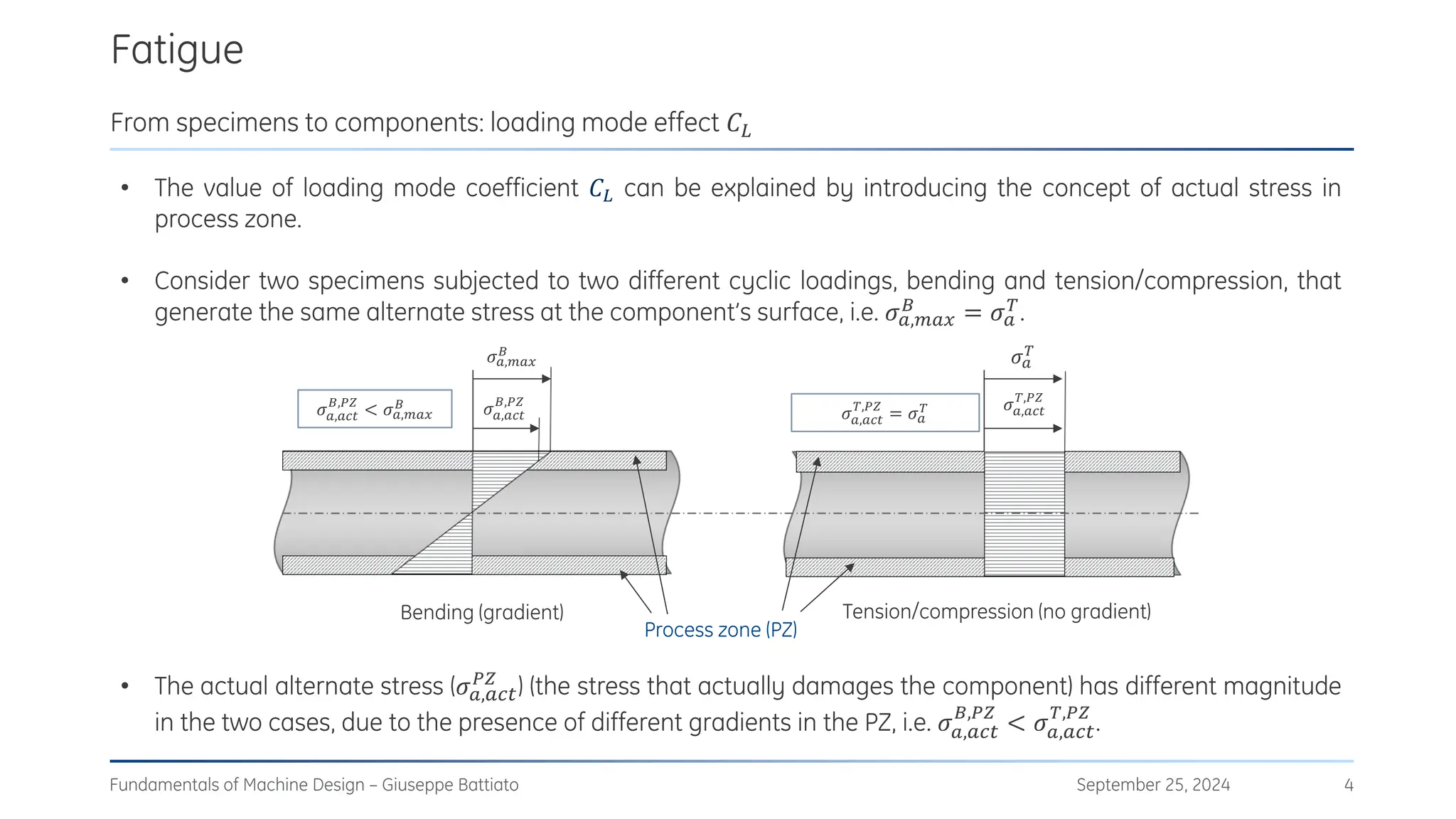
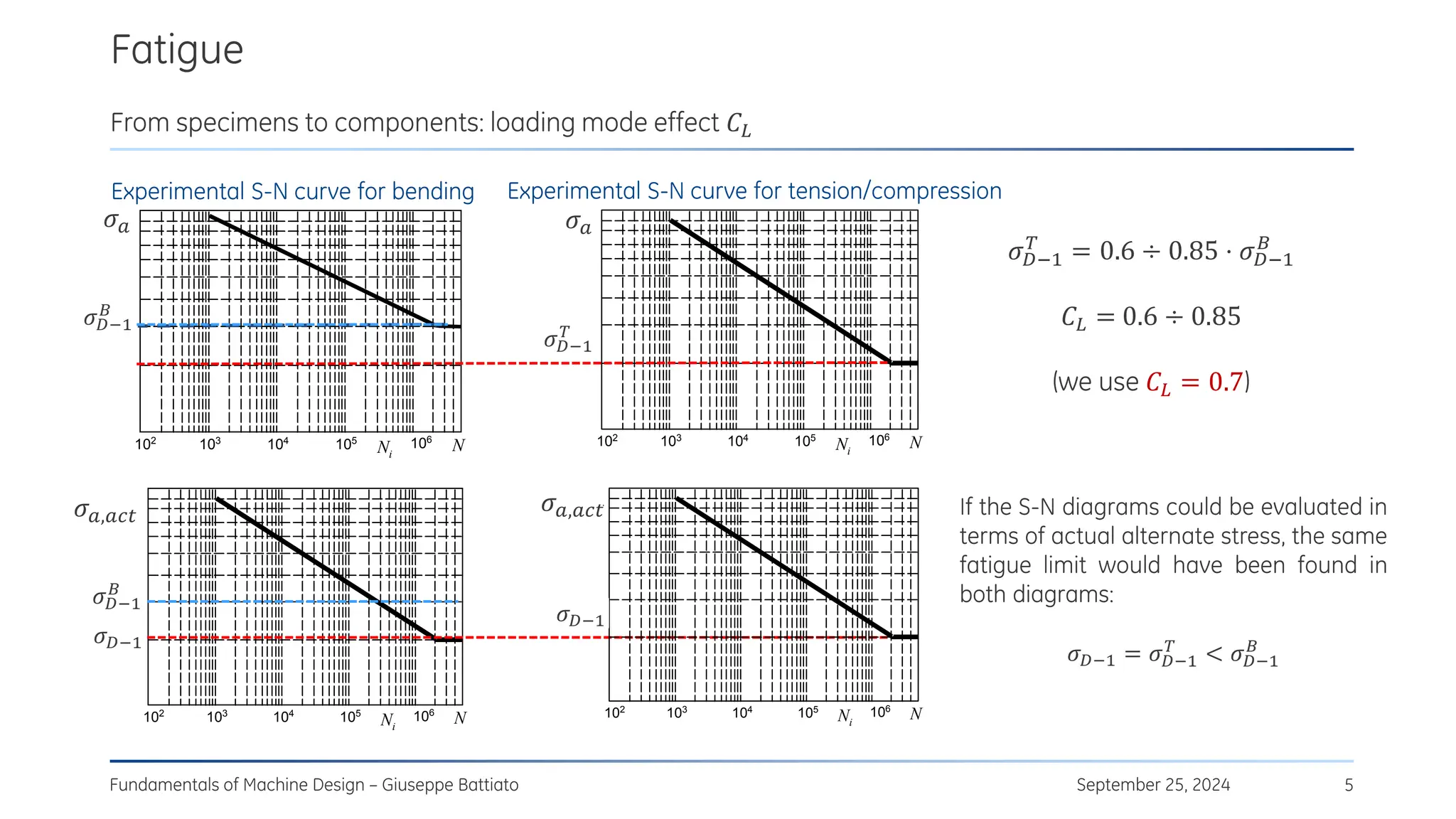
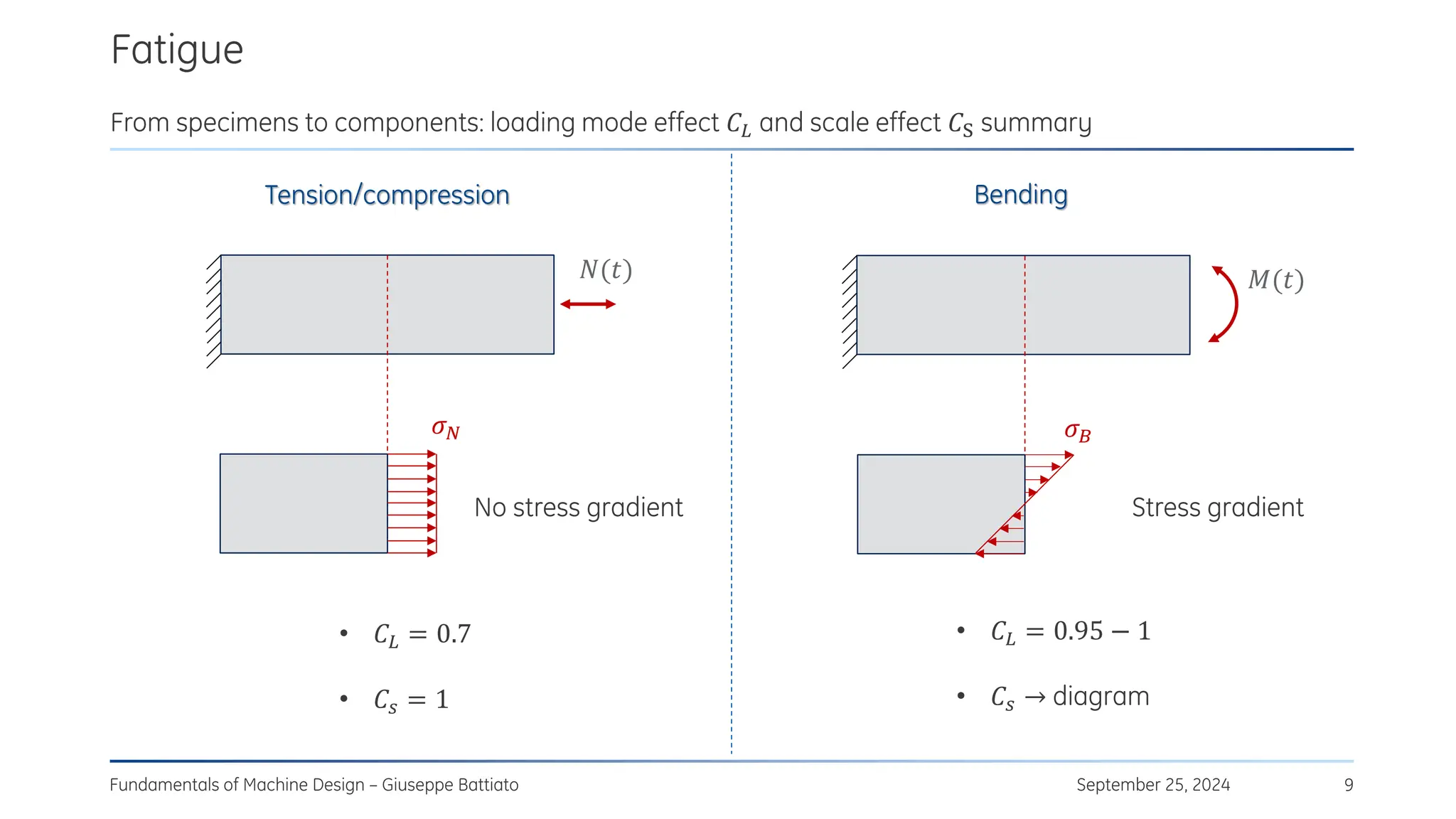
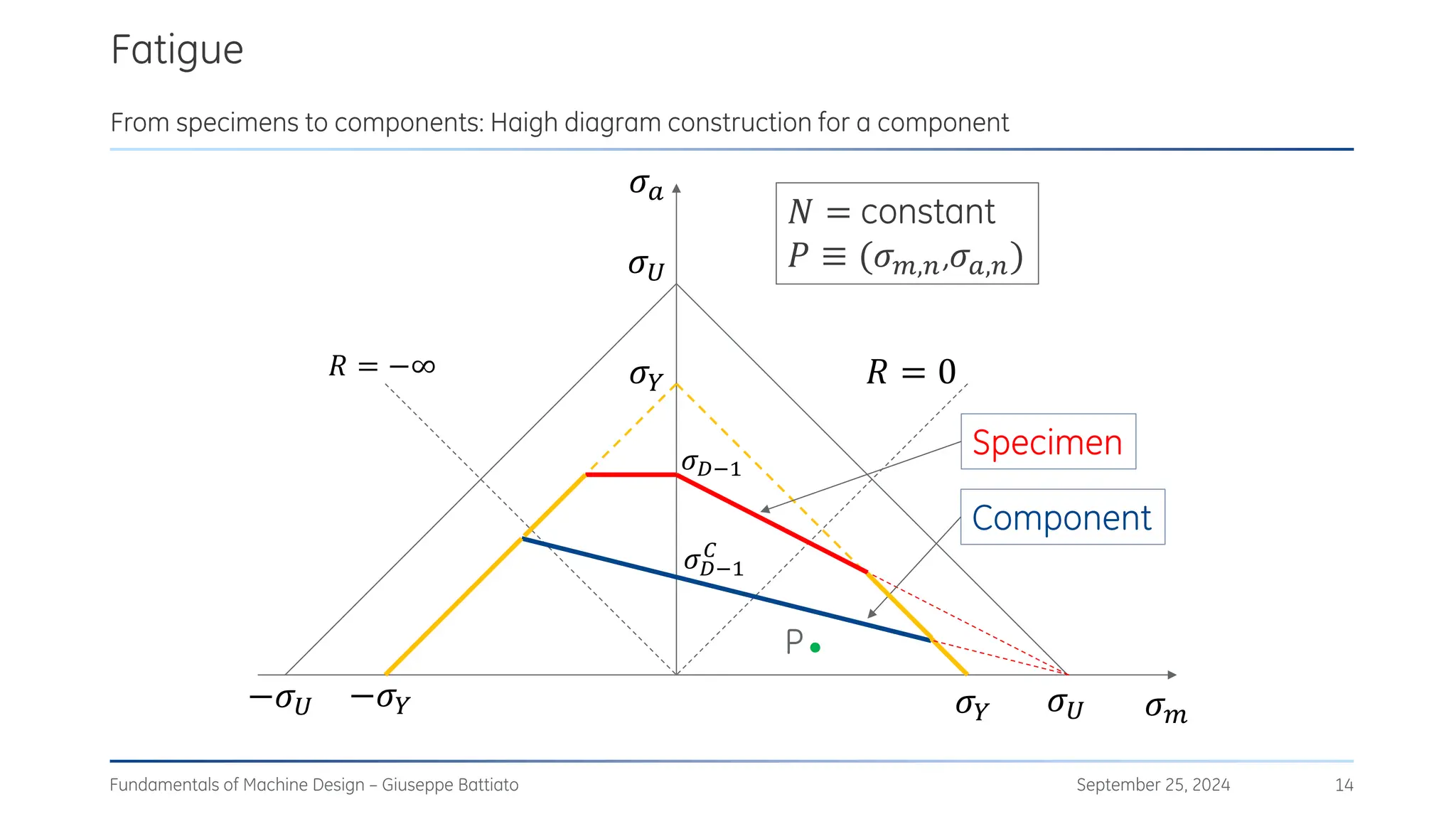
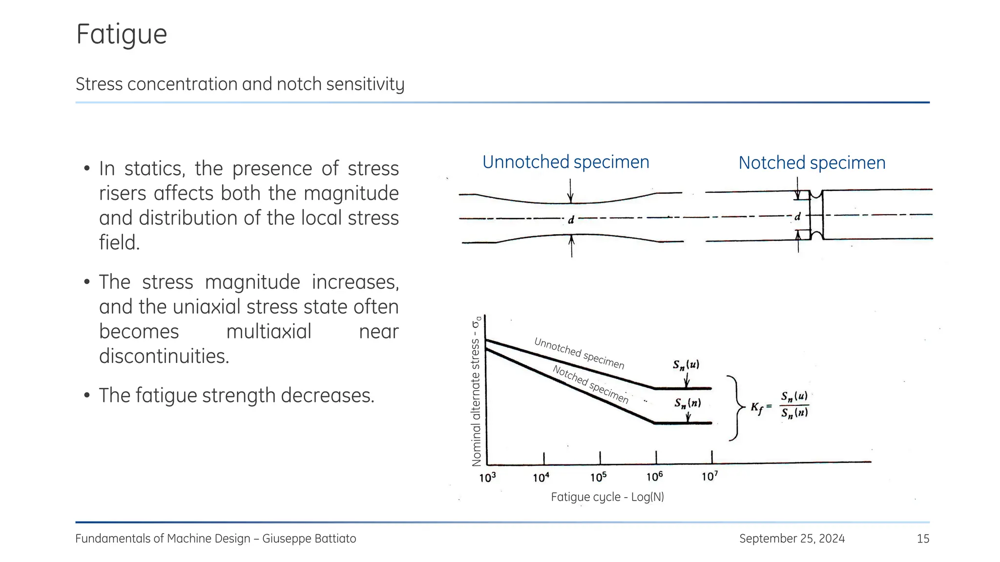
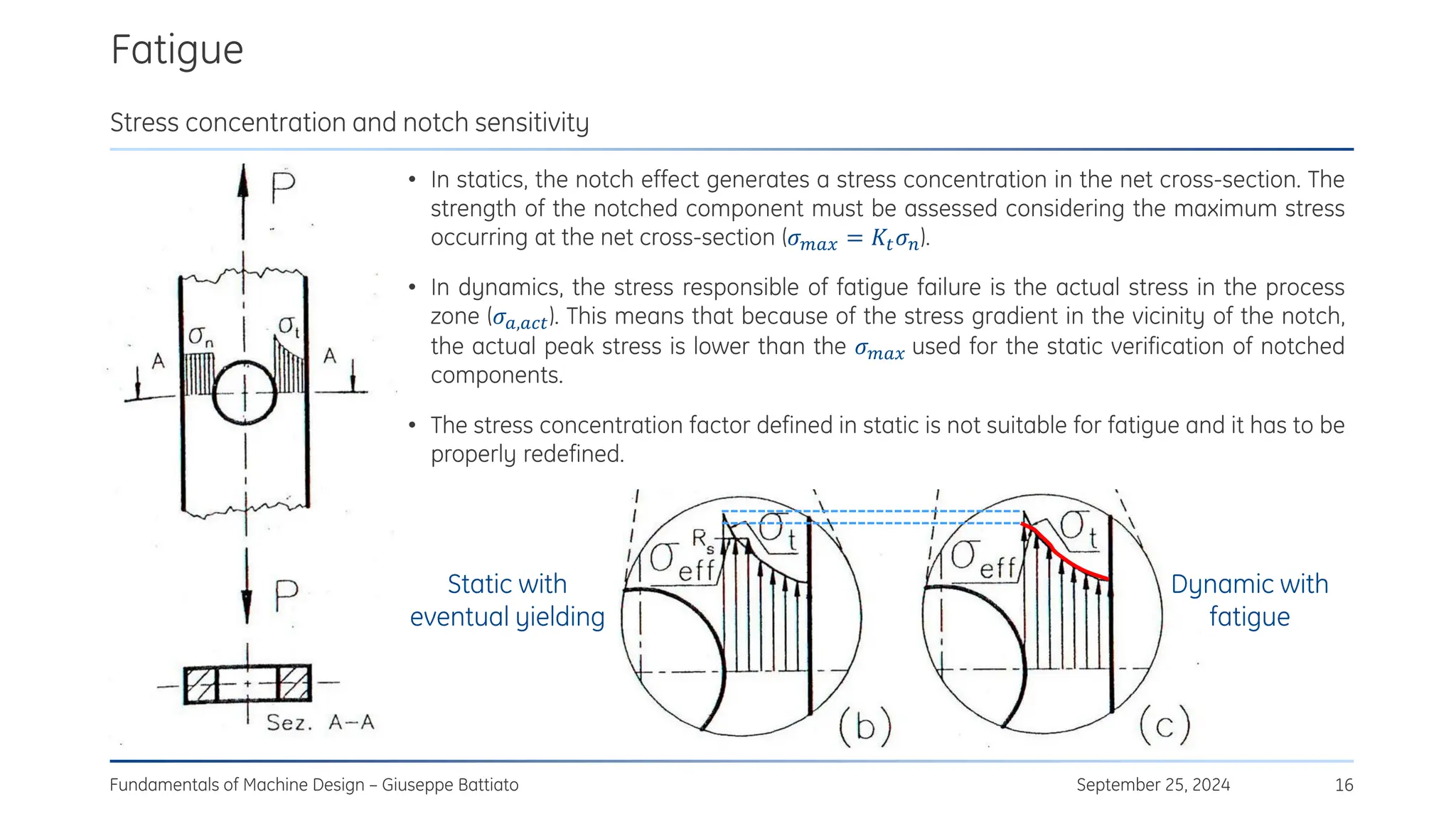
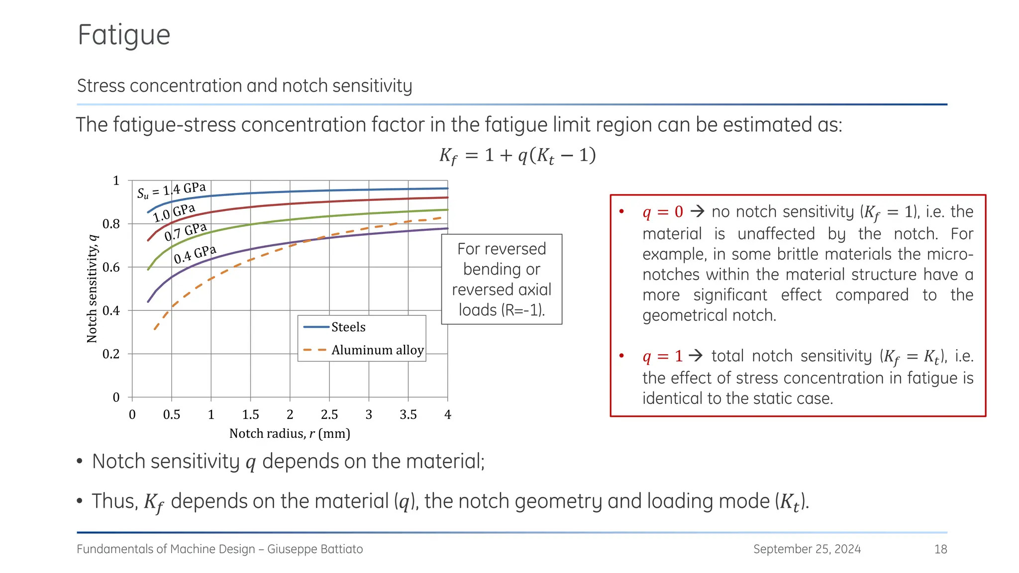
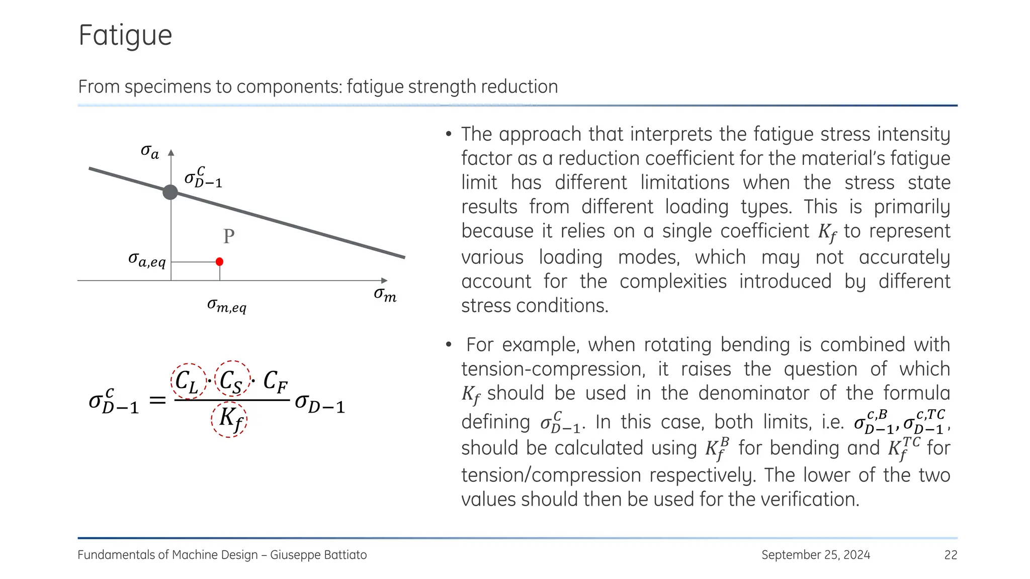
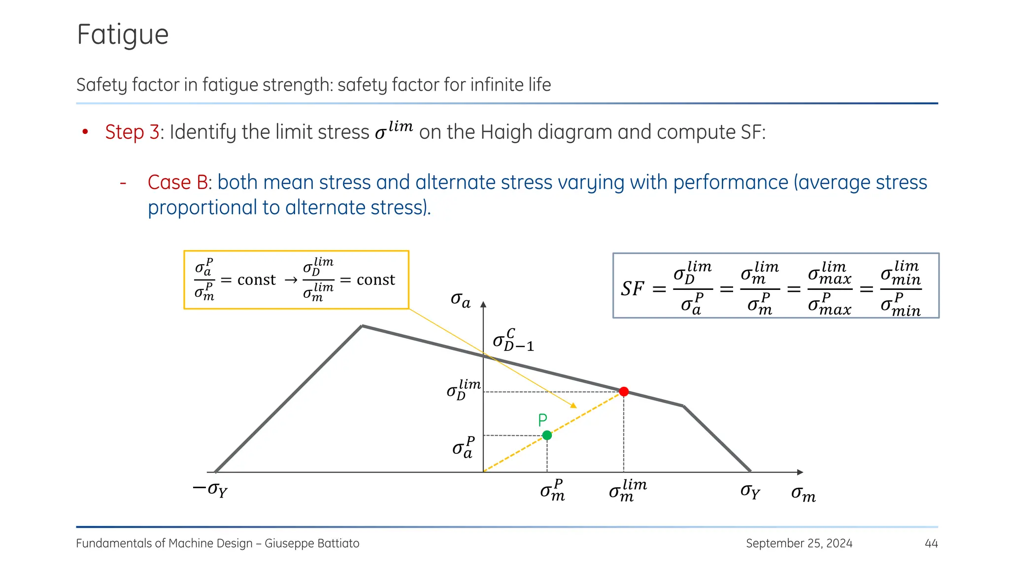
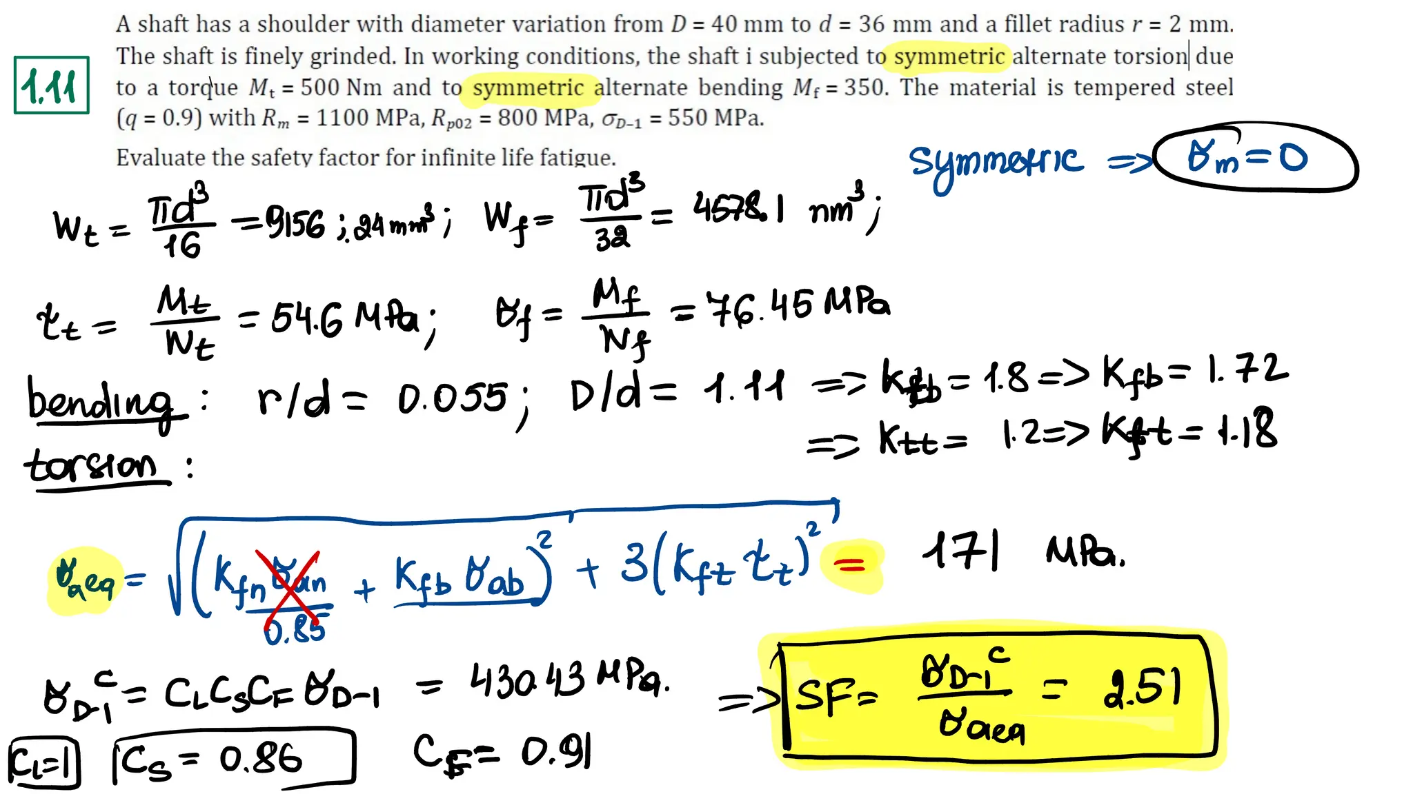
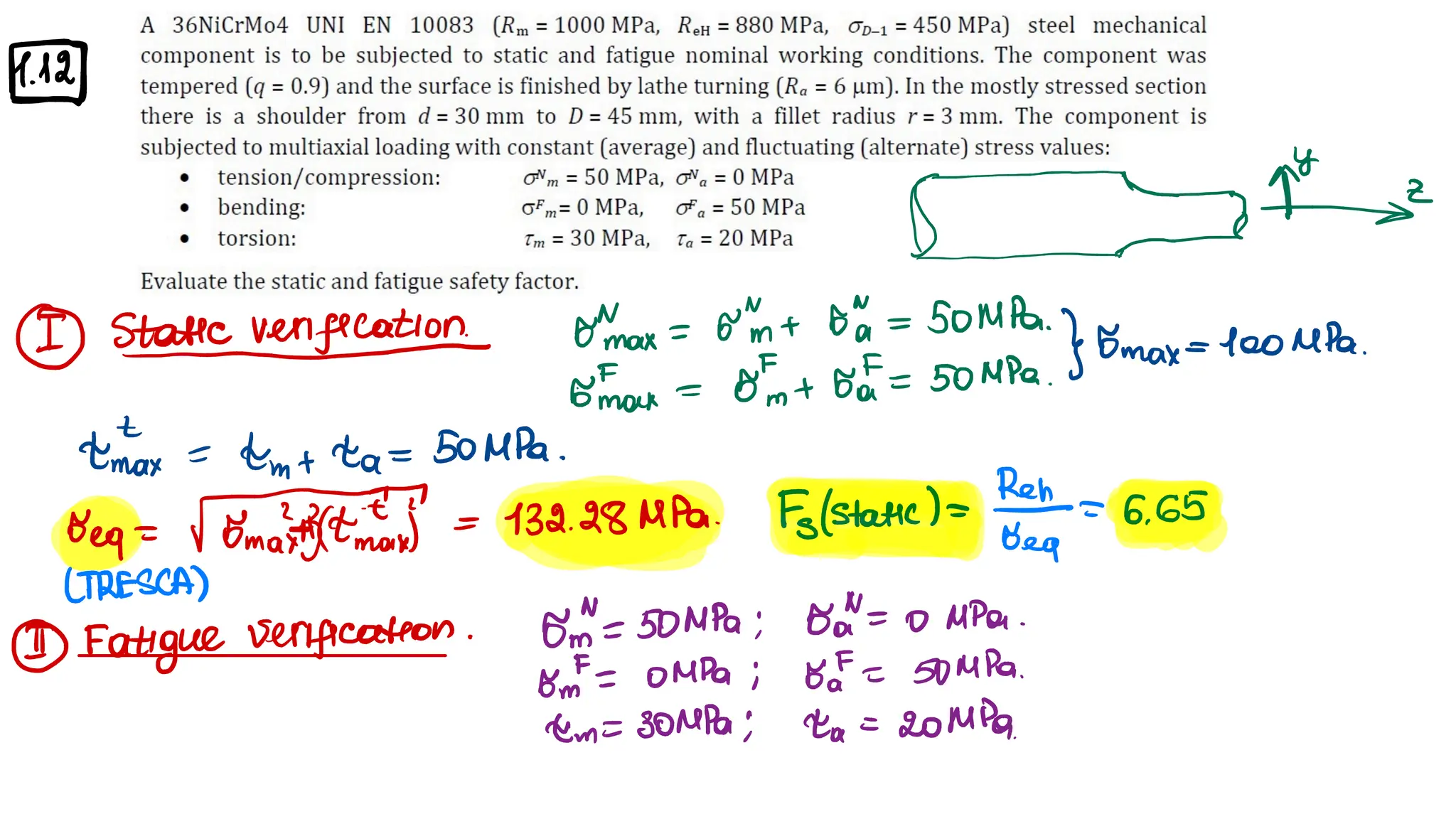
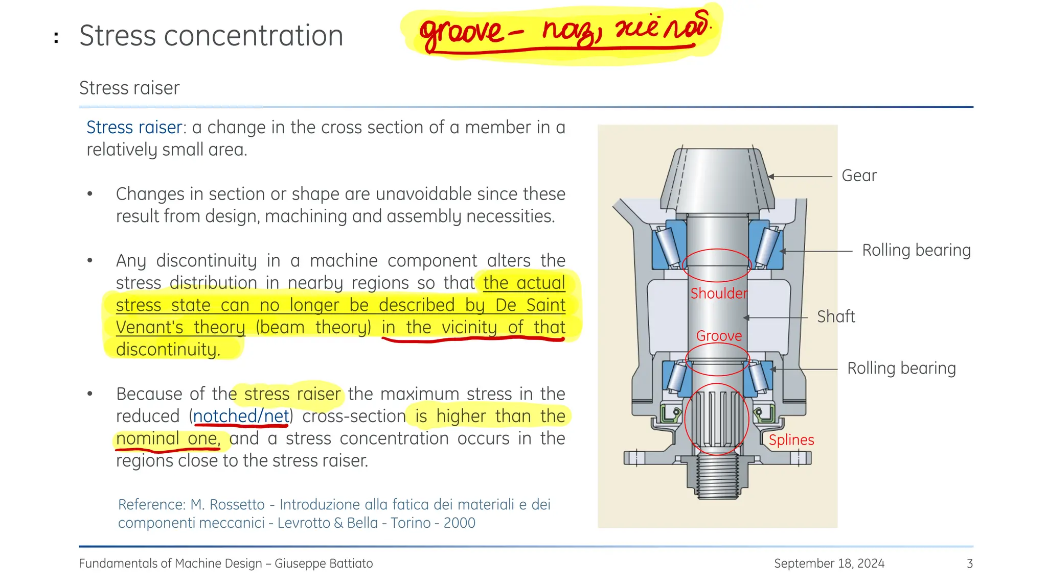
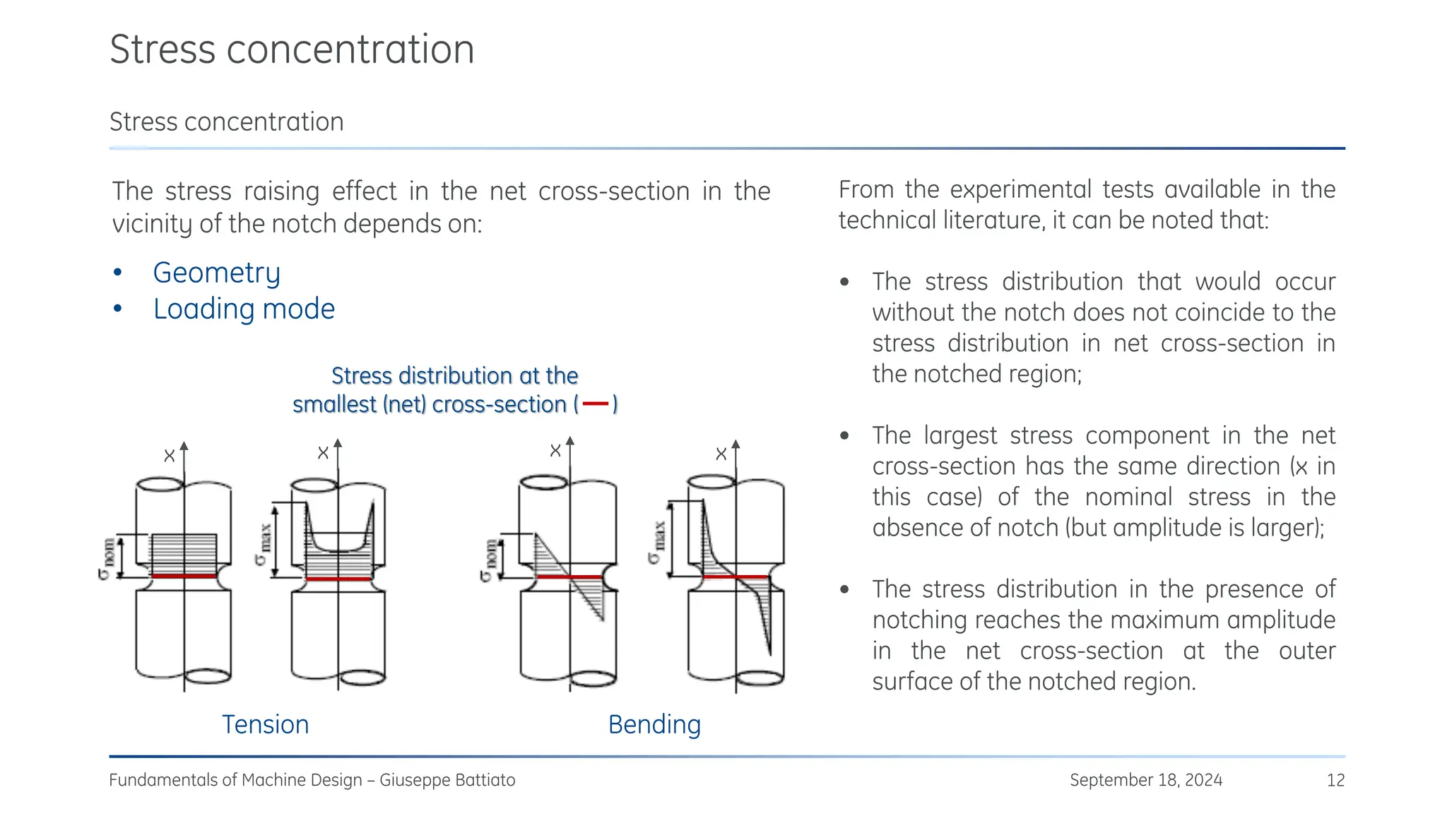
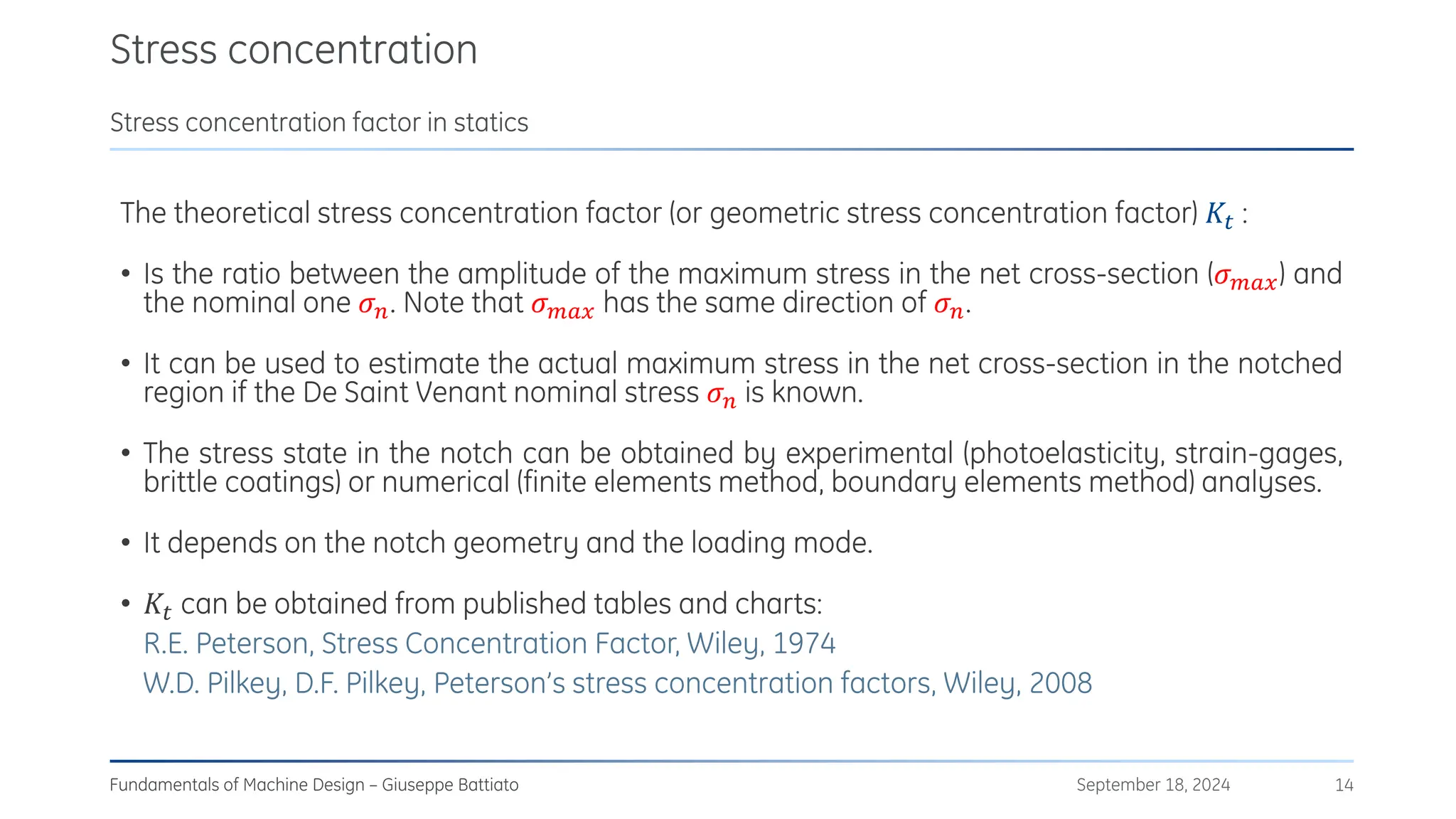
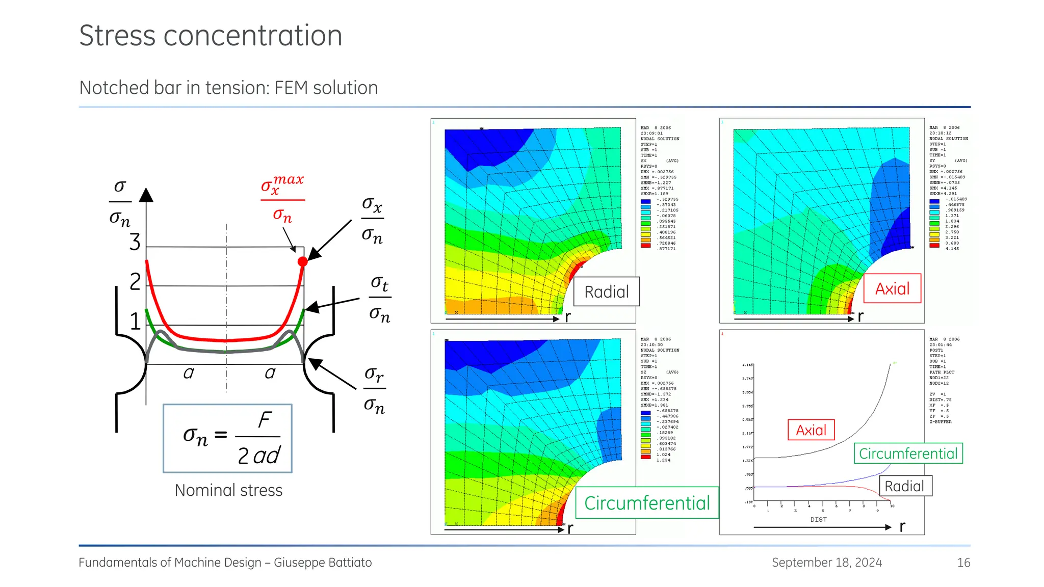
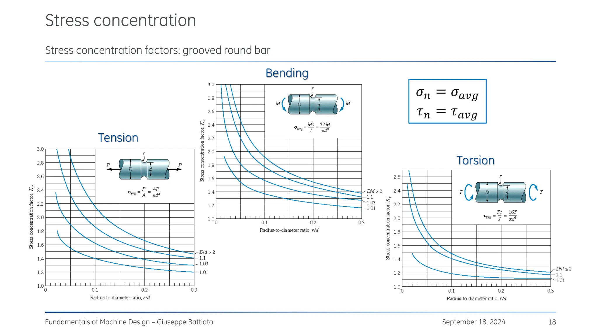
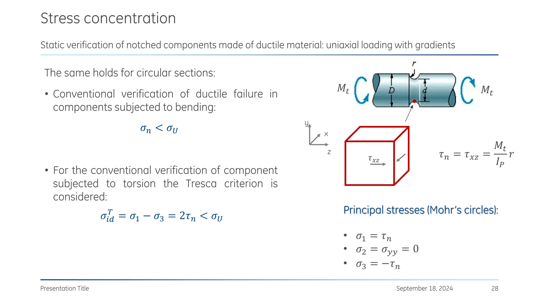
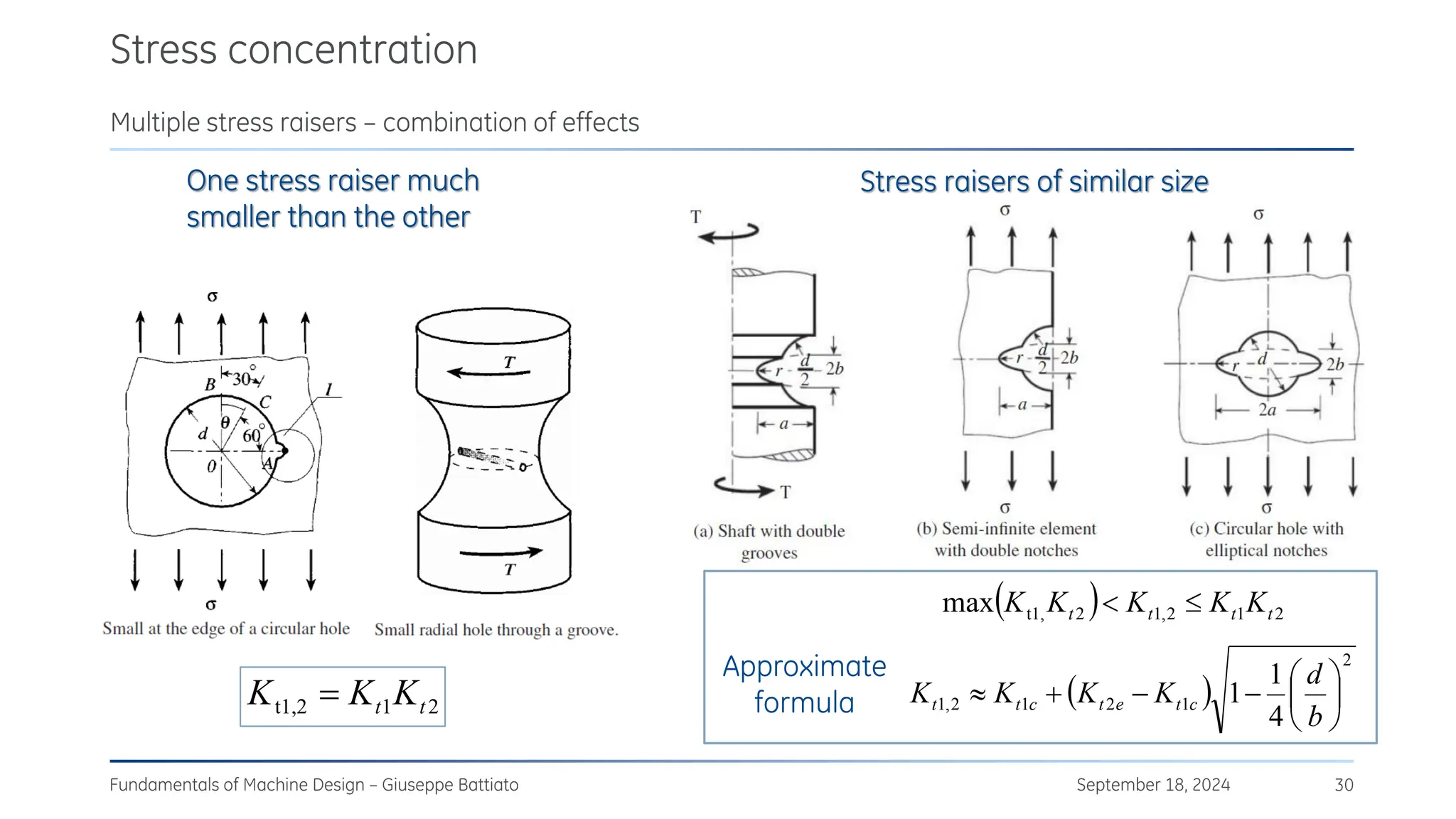
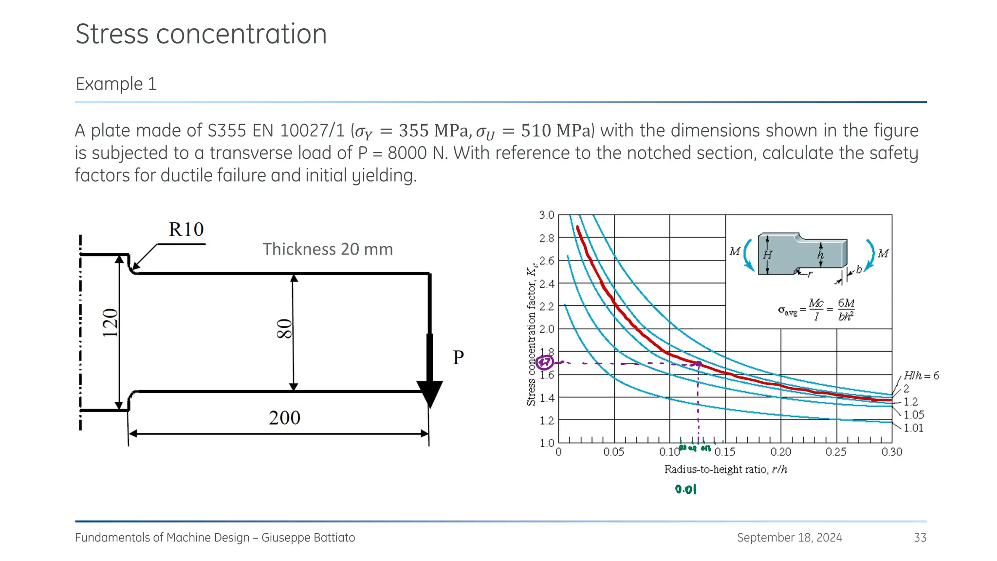
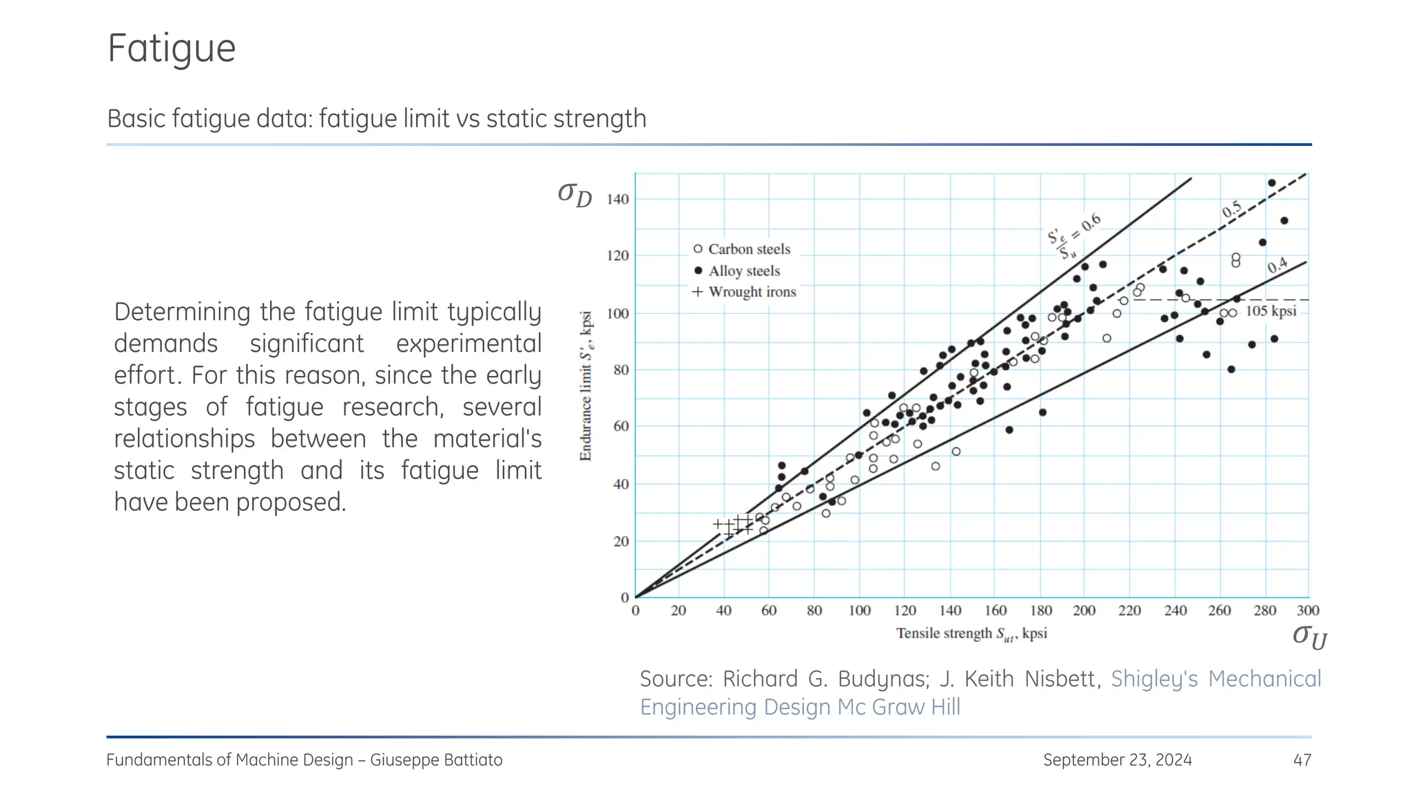
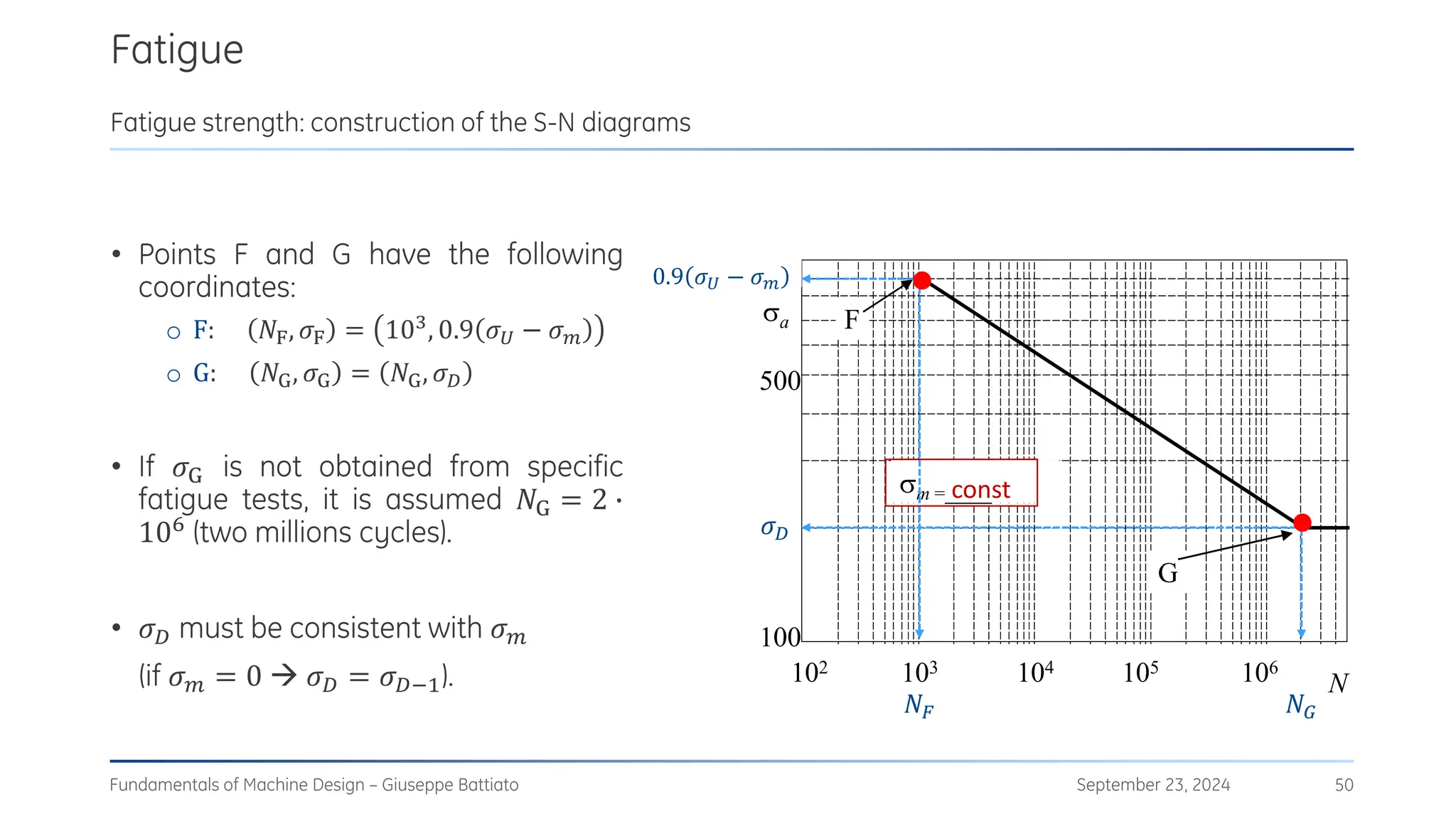
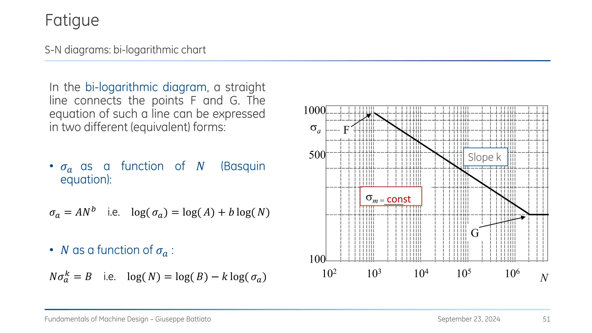
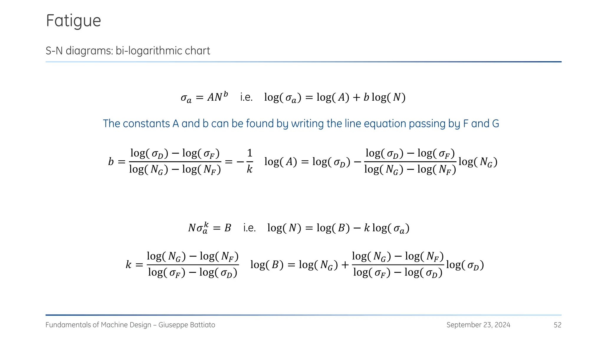
The document discusses stress concentrations in machine design, particularly focusing on stress raisers, which are areas in structural components where stress levels are significantly elevated due to geometric discontinuities, such as holes or notches. It explains how these discontinuities affect the distribution of stress and presents methods for evaluating stress concentration factors, including analytical, numerical, and experimental approaches. The document further outlines the implications of stress concentrations on ductile and brittle materials and provides guidelines for static verification of notched components.


![Fatigue
September 23, 2024
Fundamentals of Machine Design – Giuseppe Battiato 54
Exercises
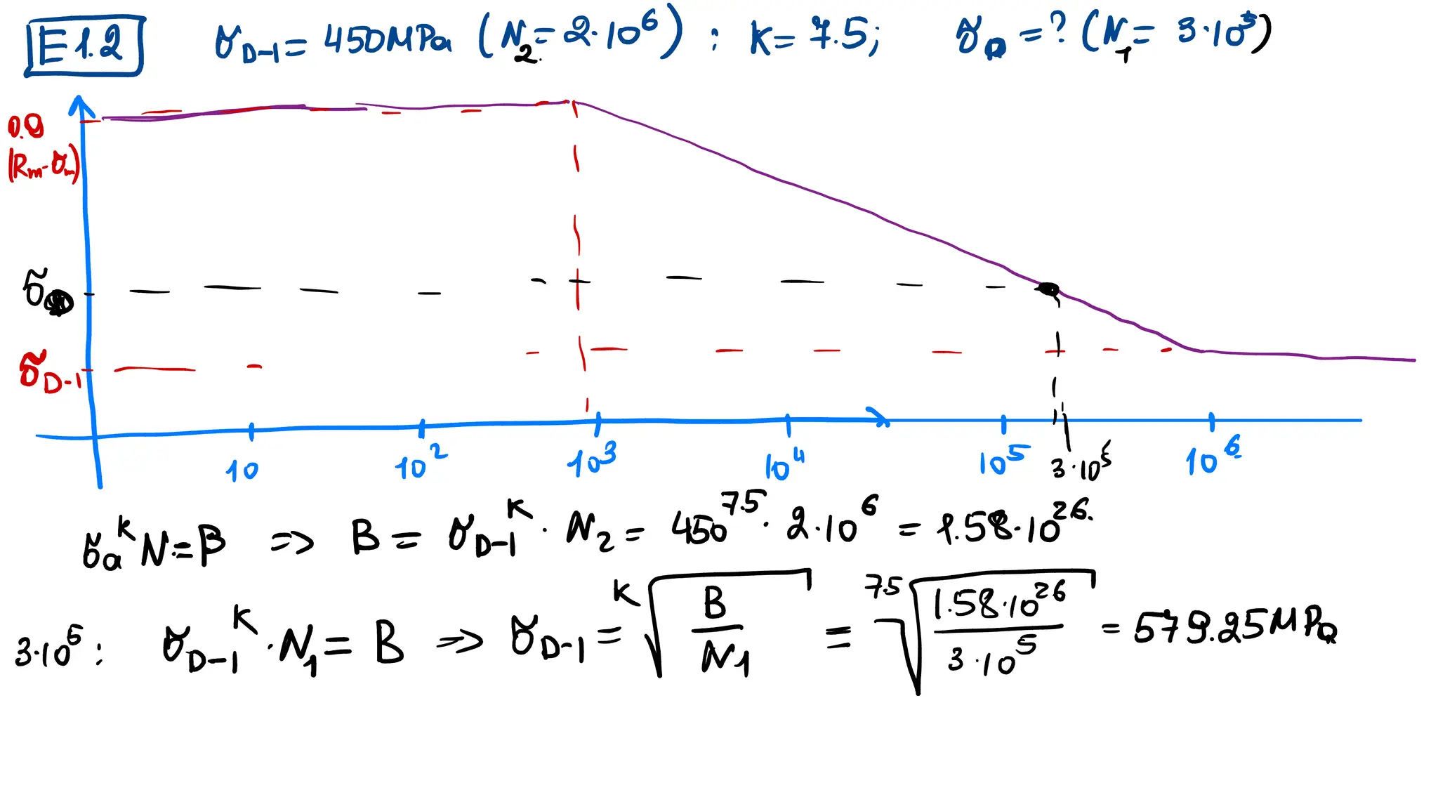
1) A material has alternate fatigue strength 𝜎𝐷−1 = 450 MPa at 𝑁∞ = 2 ∙ 106
cycles and a Wöhler curve
exponent 𝑘 = 7.5. Evaluate the alternate fatigue strength for 𝑁 = 3 ∙ 105
cycles. [𝜎𝑁 = 580 MPa]
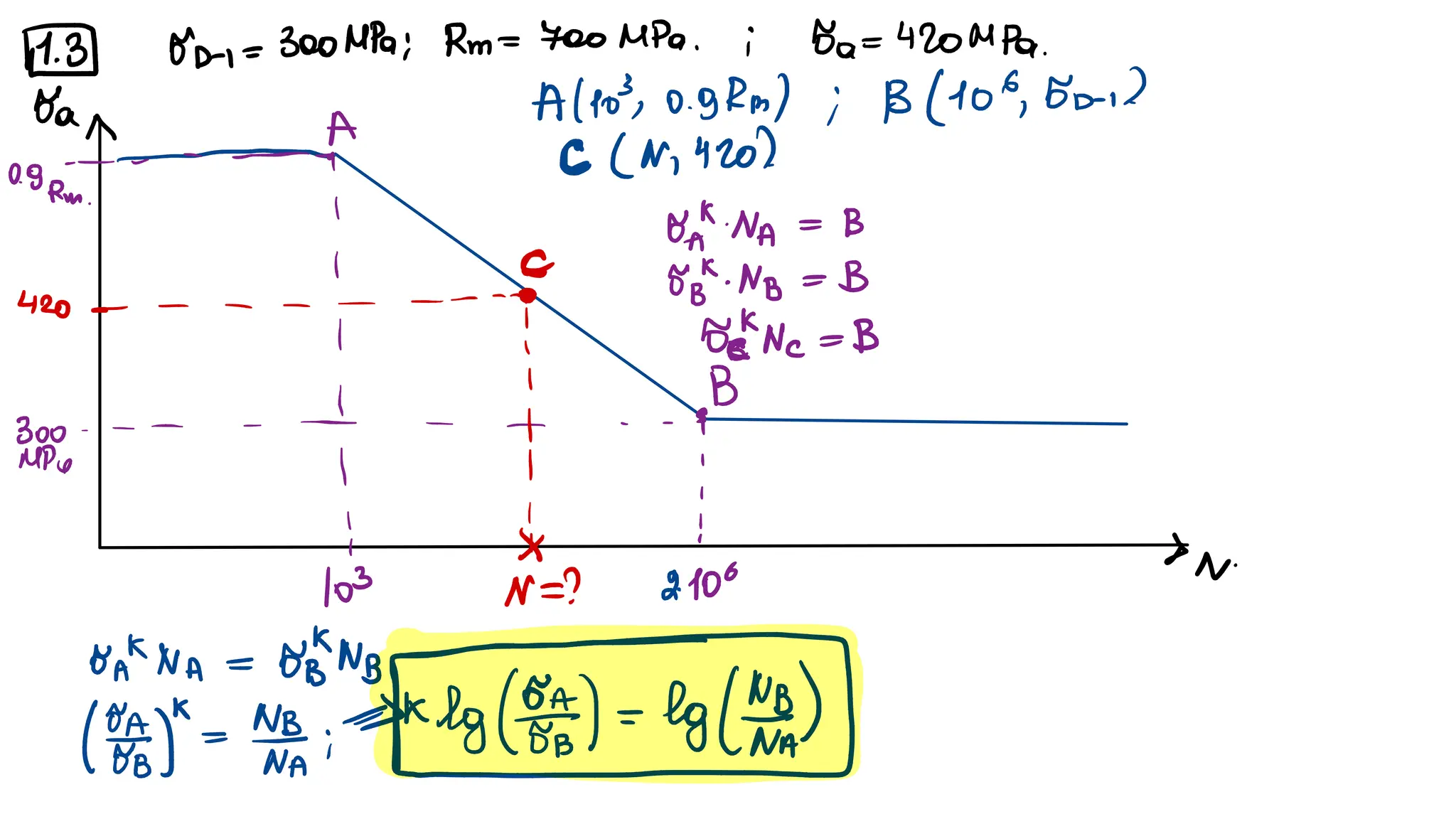
2) A specimen with 𝜎𝐷−1 = 300 MPa , 𝜎𝑈 = 700 MPa is subjected to a rotating bending moment with a
maximum value 𝜎𝑎 = 420 MPa. Evaluate the total number of cycles to failure. [𝑁 = 6.4 ∙ 104 cycles]](https://image.slidesharecdn.com/stressconcentrationfatigue-250105080615-bb01277a/75/Stress_concentration_fatigue_mechanical_-92-2048.jpg)


![Fatigue
September 23, 2024
Fundamentals of Machine Design – Giuseppe Battiato 65
Exercise
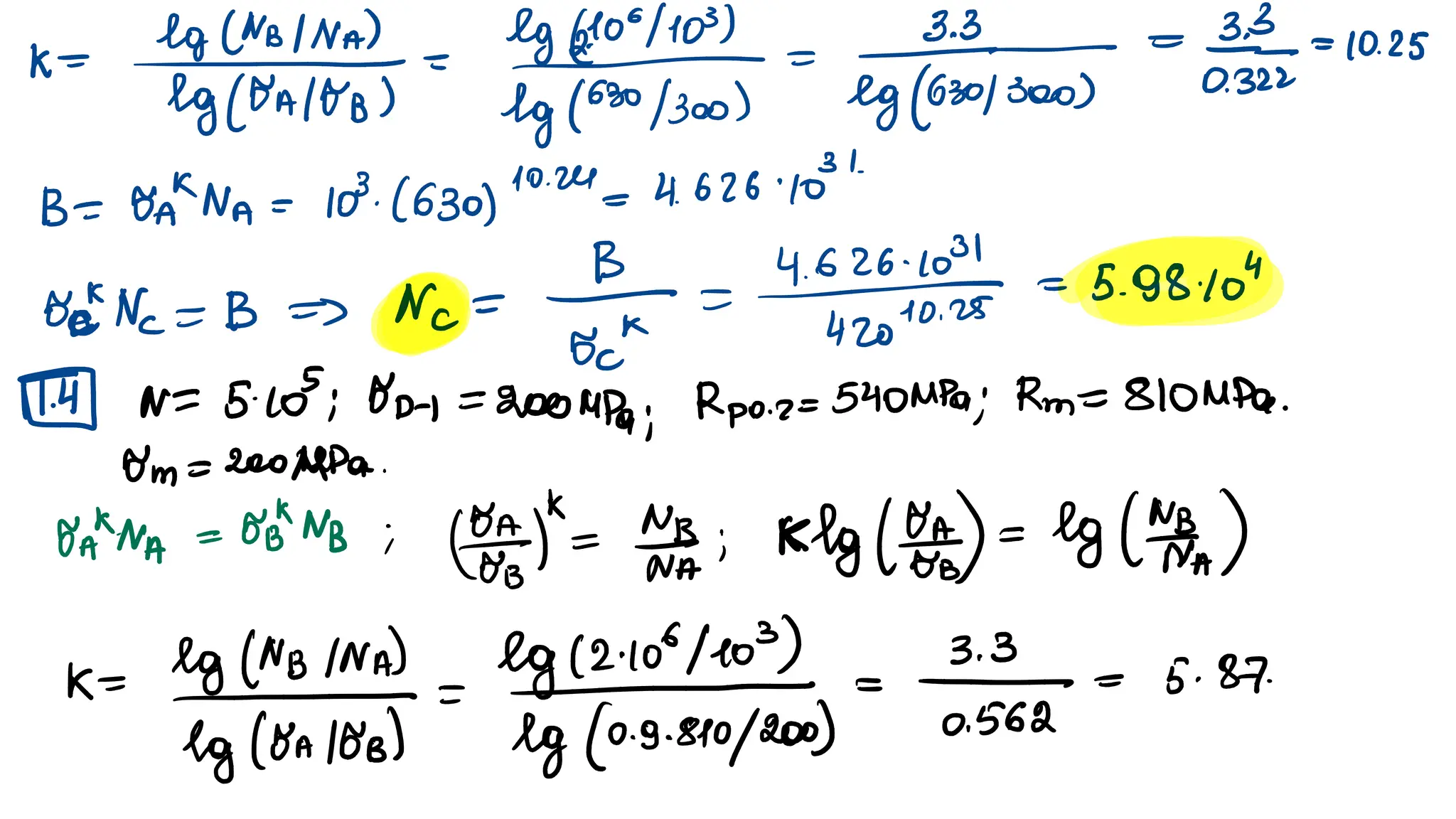
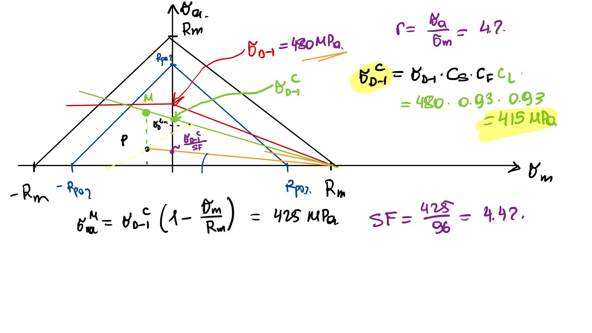
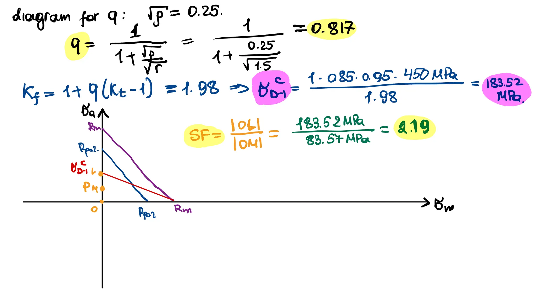
Build the Haigh diagram for a fatigue life of 𝑁 = 5 ∙ 105 cycles of a material having an alternate fatigue
limit of 𝜎𝐷−1 = 200 MPa , 𝜎𝑌 = 540 MPa , and 𝜎𝑈 = 810 MPa . Evaluate the alternate fatigue strength for
an average stress 𝜎𝑚 = 200 MPa. [𝜎𝑎 = 191 MPa ]](https://image.slidesharecdn.com/stressconcentrationfatigue-250105080615-bb01277a/75/Stress_concentration_fatigue_mechanical_-103-2048.jpg)