Downloaded 46 times


![Chapter3 14
-------------------------------------------------------------------------------------------------------------------
Commentary:
Essentially seismic design as applied to storage tanks follows the requirements prescribed by the Building
Standard Law where the importance of structures is not explicitly considered. However, as storage tanks are
more versatile than normal building structures in that they include a range of structures covering silo
containing forages and tanks for toxic materials, an importance factor, I, is introduced to accommodate these
differences. Whilst this chapter summarises the common features of seismic design for above-ground storage
tanks, specific design considerations - including the importance factor, is given in the chapters dedicated to
each principal tank design type.
1. Seismic Input
The seismic energy input, ED , the principal cause for a structure’s elasto-plastic deformation, is
approximately expressed as shown in equation (3.6.1) as follows[3.13]:
(3.6.1)
2
2
v
D
MS
E =
otations:
M total mass of a structure
Sv velocity response spectrum
The acceleration response spectrum, Sa, prescribed by the Building Standard Law, is obtained from
equation (3.6.2):
(3.6.2) gRCS ta 0=
otations:
C0 standard design shear force coefficient
Rt vibration characteristic coefficient
g acceleration of gravity
Sa and Sv are related to each other as shown in the following equation (3.6.3).
(3.6.3) va S
T
S
π2
=
otations:
T natural period for the 1st mode of a structure
Sa and Sv are indicated by broken lines in the curves shown in Figure 3.6.1, whilst the solid lines
represent the simplified curves expressed in equations (3.8) and (3.9).
Fig.3.6.1 Design Response Spectra
9.8010
2.0
1.5
1.0
0.5
Sa(m/s2
)
Sv(m/s)
5](https://image.slidesharecdn.com/storagetanks2010edition-150318021719-conversion-gate01/85/Storagetanks2010edition-20-320.jpg)


![Chapter3 25
(3.31) for
720
5672
.
F
E
.
≦
t
r
e,crccrc
.
f σ
252
1
=
where:
e,crcσ the elastic axially asymmetric buckling stress, based on
lower bound formula proposed by NASA[3.1].
The value of ecrc ,σ is given by the following equation.
(3.32)
−−−=
21
16
1
19010160
/
e,crc
t
r
exp.
r
t
E.σ
(2) Allowable bending stress crb f against the long –term overturning moment
(3.33) for 0≦
F
hσ
≦0.3
−
+=
F.
ff.
ff hcrbcr
crbcrb
σ
30
70 0
(3.34) for
F
hσ
≧0.3
−=
F
ff h
crcrb
σ
10
where:
crb f allowable bending stress against the long-time overturning
moment exclusive of internal pressure (N/mm2
)
0crf value given by eq. (3.25), (3.26) or (3.27) (N/mm2
)
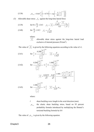
The value of crb f is given by the following equations according to the value of r/t.
(3.35) for
t
r
≦
780
2740
.
F
E
.
5.1
F
fcrb =
(3.36) for
780
2740
.
F
E
.
≦
t
r
≦
780
1062
.
F
E
.
−
+=
832.1
106.2
4.0267.0
78.0
E
F
t
r
FFfcrb
(3.37) for
780
1062
.
F
E
.
≦
t
r
ecrbcrb f ,
25.2
1
σ=
where:
e,crbσ the elastic bending buckling stress, based on lower bound
formula proposed by NASA[3.1].
The value of e,crbσ is given by the following equation](https://image.slidesharecdn.com/storagetanks2010edition-150318021719-conversion-gate01/85/Storagetanks2010edition-31-320.jpg)


![Chapter3 30
(3) In the design of silos containing granular materials, the allowable shear stress can be
calculated by setting l/r =1 and hσ =0.
Commentary:
1. Empirical formula for buckling stresses
1.1 Case without internal pressure
The lower bound values of elastic buckling stresses which apply to cylindrical shells without
internal pressures are given by the following empirical formula.
(a) elastic axial compressive buckling stresses (empirical formula by ASA[3.1])
(3.7.1)
−−=
−
t
r
eE t
r
ecrc /1901.016.0 16
1
,σ
(b) elastic flexural buckling stresses (empirical formula by ASA[3.1])
(3.7.2)
−−=
−
t
r
eE t
r
ecrb /1731.016.0 16
1
,σ
(c) elastic shear buckling stresses [3.2] [3.3]
(3.7.3)
+
×
=
t
r
t
r
r
l
t
r
r
l
E
ecr /0239.01
8.083.4
3
2,τ
Eq.(3.7.3) is given by the torsional buckling stress derived by Donnell multiplied by the reduction
factor of 0.8. These formula correspond to the 95% reliability limit of experimental data.
Based on the elastic buckling stresses, the nonlinearity of material is introduced. In the region
where the elastic buckling stresses exceeds 60% of the yield point stress of material ( yσ or yτ ),
the buckling mode is identified to be nonlinear. In Fig.3.7.1, the relationship between the buckling
stress and the r/t ratio (the buckling curve) is shown. The buckling curve in the nonlinear range is
modified as shown in Fig.3.7.1. (r/t)I is the (r/t) ratio at which the elastic buckling stress ecr,σ
reaches 60% of the yield stress. (r/t)II denotes the (r/t) ratio at which the buckling stress exceeds
the yield point stress. In the region of (r/t) ratios less than (r/t)II, the buckling stresses are assumed
to be equal to the yield point stress. In the region of (r/t) ratios between (r/t)II and (r/t)I, the
buckling stresses are assumed to be on a line as shown in the figure. (r/t)II was determined on the
condition that the elastic buckling stress at (r/t)II reaches 6.5 times to 7.5 times as large as the yield
point stress.
Fig.3.7.1 Buckling curve](https://image.slidesharecdn.com/storagetanks2010edition-150318021719-conversion-gate01/85/Storagetanks2010edition-36-320.jpg)
![Chapter3 31
(r/t)I and (r/t)II are determined according to the stress conditions as shown in Table 3.7.1.
The occurrence of buckling under combined stresses can be checked by the following criteria
(3.7.4)
=
=+
1
or
1
cr
crb
b
crc
c
τ
τ
σ
σ
σ
σ
otations:
cσ mean axial compressive stress
bσ compressive stress due to bending moment
τ shear stress
Eq.(3.7.4) implies that the axial buckling and the flexural buckling are interactive, while the shear
buckling is independent of any other buckling modes. The experimental data are shown in
Fig.3.7.2 . Figure (a) shows the data obtained by Lundquist on cylindrical shells made of
duralumin all of which buckled in the elastic range[3.4]. Figure (b) indicates the test results on
steel cylindrical shells[3.3]. The ordinate indicates crbbcrcc σσσσ // + and the abscissa indicates
crττ / . The buckling criteria which correspond to Eq.(3.7.4) is shown by the solid lines. Although
a few data can not be covered by Eq.(3.7.4), Eq.(3.7.4) should be applied as a buckling criterion
under the seismic loading considering that the estimate of Ds-values are made conservatively. For
short-term loadings other than the seismic loading, the safety factor of 1.5 is introduced in the
estimate of the elastic buckling stresses to meet the scatter of the experimental data.
Table 3.7.1 Limit r/t ratios
Stress Condition
Axial
Compression
Bending
Shearing](https://image.slidesharecdn.com/storagetanks2010edition-150318021719-conversion-gate01/85/Storagetanks2010edition-37-320.jpg)
![Chapter3 32
(a) Duralumin cylindrical shell (b) Steel cylindrical shell
Fig.3.7.2 Comparison between test results and predictions
1.2 Case with internal pressure
The effects of the internal pressure on the buckling of cylindrical shells are twofold :
・The internal pressure constrains the occurrence of buckling.
・The internal pressure accelerates the yielding of shell walls and causes the elephant foot bulge.
The effect of the internal pressure is represented by the ratio of the tensile hoop stress, hσ , to the
yield point stress, )/(, yhy σσσ [3.5].
Referring to experimental data, it was made clear that the buckling stresses under axial
compression and bending moment can be expressed by the following empirical formula[3.6] [3.7]:
(3.7.5)
−=
>
−
+=
≤
y
h
crcr
yh
yhcrcr
crcr
yh
for
for
σ
σ
σσ
σσ
σσσσ
σσ
σσ
1
,3.0/
3.0
)/)(7.0(
,3.0/
0
0
otations:
crσ buckling stress in case without internal pressure
0crσ compressive buckling stress in axi-symmetric mode
Fig.3.7.3 Influence of internal pressure on buckling stress](https://image.slidesharecdn.com/storagetanks2010edition-150318021719-conversion-gate01/85/Storagetanks2010edition-38-320.jpg)

![Chapter3 34
The applicability of Eq.(3.7.5) is demonstrated in the following:
i) Axially compressed cylinders experimental data and the results of analysis are shown in
Fig.3.7.4, together with Eq.(3.7.5) [3.7]. The abscissa indicates the hoop stress ratio, yh σσ / , and
the ordinate indicate the ratio of the buckling stress to the classical theoretical buckling stress, 1cσ .
Shell walls were perfectly clamped at both ends. Test data are indicated by the symbols of ◆ that
indicates the buckling under diamond pattern, ● that indicates the buckling under elephant foot
bulge mode and ▲ that is the case of simultaneous occurrence of diamond pattern and elephant
foot bulge mode.
Curves with a specific value of ∆ are theoretical values for elephant foot bulge mode. ∆ is the
initial imperfection divided by the thickness of wall. The chained line going up right-handedly is
the theoretical curve of diamond pattern of buckling derived by Almroth[3.8]. The polygonal line A
is the design curve for seismic loading given by Eq.(3.7.5). The polygonal line B is the design
curve for loading other than the seismic loading.
ii) Cylinders subjected to shear and bending[3.6]
Referring to experimental results on cylindrical shells subjected to shear and bending, it was made
clear that the shear buckling pattern becomes easily localized with a faint presence of the internal
pressure.
In Fig.3.7.5, a shear buckling pattern under 05.0/ =yh σσ is shown. Thus, it is understood that
the internal pressure makes the substantial aspect ratio, r/l in Eq.(3.7.3), reduced drastically.
At 3.0/ =yh σσ , the shear buckling disappears.
Considering these facts, the shear buckling stress under the internal pressure can be summarized as
follows:
(3.7.9) for 3.0/ ≤yh σσ ,
( )( )
3.0
/ yhcry
crcr
σσττ
ττ
−
+=
for 3.0/ >yh σσ , ycr ττ =
otations:
yτ shear yield-point stress
Fig.3.7.5 Buckling wave pattern of shear buckling
2
/3.32,0.1/,477/,05.0/ cmkrtr yyh ==== σσσ l](https://image.slidesharecdn.com/storagetanks2010edition-150318021719-conversion-gate01/85/Storagetanks2010edition-40-320.jpg)


![Chapter3 37
[3.3] [3.6] [3.10] [3.11].
The hysteretic behavior of cylindrical shells under repeated horizontal forces is shown in
Fig.(3.7.9).
The basic rule which governs the hysteretic behavior is described as follows.
・ Definitions to describe the hysteretic rule:
a) The loading path is defined by 0>θσdb .
b) The unloading path is defined by 0<θσdb .
・ The θσ −b relationship under the monotonic loading is defined to be the skeleton curve.
・ The unloading point is defined to be the point which rests on the skeleton curve and
terminates the loading path.
・ The initial unloading point is defined to be the point at which the buckling starts.
・ The intermediate unloading point is defined to be the point which does not rest on the
skeleton curve and terminates the loading path.
On the assumption that the loading which reaches the initial loading point has been already made
in both positive and negative directions, the hysteretic rule is described as follows.
a) The loading path points the previous unloading point in the same loading domain. After
reaching the previous unloading point, the loading path traces the skeleton curve.
b) The unloading path from the unloading point points the initial unloading point in the
opposite side of loading domain. The unloading path from the intermediate unloading point
has a slope same as that of the unloading path from the previous unloading point in the same
loading domain.
These hysteretic rule has been ascertained to apply even for the case of 0/ ≠yh σσ .
Fig.3.7.8 Load-deformation relationship under monotonic loading
Fig.3.7.9 Hysteretic rule
skeleton curve
loading path
unloading path
initial unloading point
unloading point
intermediate unloading point
parallel](https://image.slidesharecdn.com/storagetanks2010edition-150318021719-conversion-gate01/85/Storagetanks2010edition-43-320.jpg)
![Chapter3 38
5. ηD -values for cylindrical structures
ηD -values for structures with short natural periods which has been obtained analytically using
the load-deformation characteristics shown in Fig.3.7.9 are shown in Fig.3.7.10[3.12].
Essential points in the analysis are summarized as follows.
5.1 ηD -values in case that uplift of the bottom of the structure is not allowed by restraint of an
anchoring system:
1) Assuming that the structure is one-mass system and equating the structural energy
absorption capacity to the energy input exerted by the earthquake, the maximum deformation
of the structure is obtained.
2) The energy input to the structure is obtained by considering the elongation of the vibrational
period of structure.
3) The ηD -values is defined by
(3.7.11)
cr
cr
D
δµ
δ
η
)1(ofndeformatiomaximumthecauseswhichearthquakeoflevelthe
n,deformatiobucklingthecauseswhichearthquakeoflevelthe
+
=
otations:
1−=
cr
m
δ
δ
µ nondimensionalized maximum deformation
crδ buckling deformation
4) The assumed load-deformation curve in monotonic loading is one that exhibits a
conspicuous degrading in strength in the post-buckling range as shown in Fig.3.7.10. q in
the figure denotes the nondimensionalized level of the stationary strength in the post buckling
range.
When we select the value of ηD to be 0.5, the pairs of values of ( µ,q ) are read from
Fig.3.7.10 as follows : (0.6, 1.0), (0.5, 2.0), and (0.4, 4.0). See Table 3.7.3.
These µ−q relationships which corresponds to 5.0=ηD are compared with the
nondimentionalized load-deformation curves obtained experimentally in Fig.3.7.11 and
Fig.3.7.12. The µ−q relations are written as white circles in these figures. The
experimental curves lie almost above the µ−q relations for 5.0=ηD (see Table 3.7.3). It
implies that the actual structures are more abundant in energy absorption capacity than the
analytical model equipped with the load-deformation characteristics shown in Fig.3.7.10.
Thus, to apply the value of 0.5 for ηD -values of cylindrical structures influenced by buckling
seems reasonable. When the axial compressive stress becomes large, however, the ηD -
values should be kept larger than 0.5 since the strength decreases drastically in the post
buckling range.
Consequently, the value of ηD is determined as follows:](https://image.slidesharecdn.com/storagetanks2010edition-150318021719-conversion-gate01/85/Storagetanks2010edition-44-320.jpg)
![Chapter3 39
Fig.3.7.10 ηD -values
for crcσσ /0 ≦0.2,
(3.7.12) 5.0=ηD
for crcσσ /0 >0.2,
(3.7.13) 7.0=ηD
Table 3.7.3 q(=Q/Qcr) and )/][( crcr δδδµ −= relationship (in case of 2.0/0 ≦crδδ , 5.0=ηD )
q µ
0.6 1.0
0.5 2.0
0.4 4.0
Fig.3.7.11 Load-deformation relationship
which corresponds to 5.0=ηD
( 0/ =yh σσ )](https://image.slidesharecdn.com/storagetanks2010edition-150318021719-conversion-gate01/85/Storagetanks2010edition-45-320.jpg)


![Chapter3 43
(a) Seismic active earth pressure resultant
(3.8.1) 2
)
cos2
)(1(' HK
H
KP EAVEA
θ
ωγ
+−=
(b) Seismic passive earth pressure resultant
(3.8.2) 2
)
cos2
)(1(' HK
H
KP EPVEP
θ
ωγ
+−=
where:
'EAP seismic active earth pressure resultant acting on the wall
with depth H ( /mm)
EAK see eq. (3.64) in chap. 3.8.2
VK see eq. (3.15) in chap. 3.6.2.2
γ unit weight of soil ( /mm3
)
H depth from the ground surface to the tank bottom (mm)
ω imposed loads ( /mm2
)
θ seismic composite angle (=tan-1
K)
'EPP seismic passive earth pressure resultant acting on the wall
with depth H ( /mm)
EPK see equation (3.66) in chap. 3.8.2
As shown above, Mononobe and Okabe’s formula gives the resultant acting on the tank wall for a
unit width soil wedge above the slip surface. For convenience, this recommendation transforms
equations (3.8.1) and (3.8.2) to pressures per unit area of the tank wall as in equations (3.63) and
(3.65). If these equations are integrated in the interval z = 0~H, equations (3.8.1) and (3.8.2) will
be obtained.
Equations (3.63) ~ (3.66) give pressures acting in the inclined direction with angle δ from the
horizontal plane. But the angle of friction between the wall and the soil may be neglected, and the
pressures may be regarded as acting in the normal direction to the wall.
The equations in this chapter give ultimate earth pressure, but they have limitations in that their
basis is static equilibrium and they depend on assumed seismic intensity. Therefore additional
methods, such as response displacement, seismic intensity, or dynamic analysis methods should
also be used in the design for seismic loads.
References:
[3.1] ASA SP-8007: Buckling of Thin-walled Circular Cylinders, Aug. 1968
[3.2] Donnell, L. H.: Stability of Thin-walled Tubes under Torsion, ACA, T 479, 1933
[3.3] Akiyama, H., Takahashi, M., Hashimoto, S.: Buckling Tests of Steel Cylindrical Shells Subjected to
Combined Shear and Bending, Trans. of Architectural Institute of Japan, Vol. 371, 1987
[3.4] Lundquist, E. E.: Strength Test of Thin-walled Duralumin Cylinders in Combined Transverse Shear and
Bending, ACA, T 523, 1935
[3.5] Yamada, M.: Elephant's Foot Bulge of Cylindrical Steel Tank Shells JHPI, Vol. 18, o. 6, 1980
[3.6] Akiyama, H., Takahashi, M., omura, S.: Buckling Tests of Steel Cylindrical Shells Subjected to
Combined Bending, Shear and Internal Pressure, Trans. of Architectural Institute of Japan, Vol. 400,
1989
[3.7] Yamada, M., Tsuji, T.: Large Deflection Behavior after Elephant's Foot Bulge of Circular Cylindrical
Shells under Axial Compression and Internal Pressure
Summaries of Technical Papers of Annual Meeting, AIJ, Structure-B, pp. 1295-1296, 1988
[3.8] Almroth Bo O., Brush D. O.: Postbuckling Behavior of Pressure Core-Stabilized Cylinders under Axial
Compression. AIAA J., Vol. 1, pp.2338-2441, 1963](https://image.slidesharecdn.com/storagetanks2010edition-150318021719-conversion-gate01/85/Storagetanks2010edition-49-320.jpg)
![Chapter3 44
[3.9] Yamada, M.: Elephant's Foot Bulge of Circular Cylindrical Shells
The Architectural Reports of the Tohoku University, Vol. 20, pp. 105-120, 1980
[3.10] Shibata, K., Kitagawa, H., Sampei, T. Misaji, K: The Vibration Characteristics and Analysis of After
Buckling in Metal Silos, Trans. of Architectural Institute of Japan, Vol. 367, 1986
[3.11] Kitagawa, H., Shibata, K.: Studies on Comparison of Earthquake - Proof of Metal and FRP Silos,
Summaries of Technical Papers of Annual Meeting, AIJ, Structure - B, 1988
[3.12] Akiyama, H.: Post Buckling Behavior of Cylindrical Structures Subjected to Earthquakes, 9th SMiRT,
Lausanne, 1987
[3.13] Kato, B., Akiyama, H.: Energy Input and Damages in Structures Subjected to Severe Earthquakes,
Trans. of Architectural Institute of Japan, Vol. 235, 1975](https://image.slidesharecdn.com/storagetanks2010edition-150318021719-conversion-gate01/85/Storagetanks2010edition-50-320.jpg)


![Chapter 5 62
The calculation of stresses on the parts of the silo during earthquakes should be
based on the requirements of section 3.7.4.
The calculation of short-term stresses on parts caused by other than earthquakes
should be based on section 3.7.3.
5.4.2 Design of Hopper Walls
The axial stress on the section of the hopper wall in the direction of generator, σφ ,
and the tensile stress in the circumferential direction, σθ , are calculated using
equations (5.15) and (5.16) respectively.
(5.15)
( )
t
v
c
sh
f
sint
ddP
sintl
WW
≤
⋅⋅
′⋅
+
⋅⋅
+
=
αα
σφ
22 4
(5.16) t
a
f
sint
ddP
≤
⋅⋅
′⋅
=
α
σθ
22
where:
Wh weight of the contents of the hopper beneath the section (N)
Ws weight of the hopper beneath the section (N)
t2 wall thickness of the hopper (mm)
lc perimeter of the hopper at the section level (mm)
d’ diameter of the hopper wall at the section level (mm)
α inclination of the hopper wall (degree)
dPv vertical design pressure per unit area at the section level (N/mm2
)
dPa perpendicular design pressure per unit area on the hopper wall at the
section level (N/mm2
)
ft allowable tensile stress (N/mm2
)
5.4.3 Design of Supports
Local bending stresses should be considered in design procedure that may act on the
connections between the hopper or machines and their supports or other similar parts.
References:
[5.1] International Standard : ISO 11697, Bases for Design of Structures – Loads due to Bulk Materials,
1995.6
[5.2] American Concrete Institute : Standard Practice for Design and Construction of Concrete Silos and
Stacking Tubes for Storing Granular Materials (ACI 313-97) and Commentary—ACI 313R-97,
1997.1
[5.3] Australian Standard : Loads on Bulk Solids Containers (AS 3774-1996), 1996.10
[5.4] Janssen, H.A. : Versuche berU&& Getreidedruck in Silozellen : VID Zeitschrift (Dusseldorf) V. 39, pp.
1047~1049, 1885.8
[5.5] aito, Y., Miyazumi, K., Ogawa, K., akai, . : Overpressure Factor Based on a Measurement of a
Large - scale Coal Silo during Filling and Discharge, Proceedings of the 8th International
Conference on Bulk Materials Storage, Handling and Transportation (ICBMH’04), pp. 429 – 435,
2004.7
[5.6] Ishikawa, T., Yoshida, J. : Load Evaluation Based on the Stress Measurement in a Huge Coal Silo (in
Japanese), Journal of Structural and Construction Engineering (Transactions of AIJ), o.560, pp.
221 – 228, 2002.10](https://image.slidesharecdn.com/storagetanks2010edition-150318021719-conversion-gate01/85/Storagetanks2010edition-68-320.jpg)
![Chapter 5 63
[5.7] S.P. Timoshenko and S.W. Kreiger : Theory of Plates and Shells, McGraw-Hill, 1959
[5.8] G.E. Blight : A Comparison of Measured Pressures in Silos with Code Recommendations, Bulk
Solids Handling Vol. 8, o. 2, pp. 145~153, 1988.4
[5.9] J.E. Sadler, F. T. Johnston, M. H. Mahmoud : Designing Silo Walls for Flow Patterns, ACI
Structral Journal, March-April 1995, pp. 219~228 (Title o. 92-S21), 1995
[5.10] A.W. Jenike: Storage and Flow of Solid, Bulletin o. 123 of the Utah Engineering Experiment
Station, University of Utah, 1964.11](https://image.slidesharecdn.com/storagetanks2010edition-150318021719-conversion-gate01/85/Storagetanks2010edition-69-320.jpg)


![Chapter 6 69
weight imposed on the base of the structure W is calculated as the sum of WD , and f(ξ) WI . The
weight ratio of the impulsive mass of the tank contents, f(ξ), is determined with reference to
experimental data of the vibration of a real scale structure [6.1] [6.2].
The structural characteristic coefficient, Ds , is obtained from equation (6.3) which is based on the
mean cumulative plastic deformation ratio of the supporting structure, η, (see Commentary 3.6.1),
which is obtained from equation (6.4). This equation assumes that δm is the horizontal
displacement of the column head when a supporting column reaches the short-term allowable
strength, that δy is the horizontal displacement of the column head when a bracing reaches the
short-term allowable strength, and δm - δy is the mean cumulative plastic deformation. When the
allowable strength of the bracing is governed by a buckling, i.e., when T < 2 C , the energy
absorption capacity (deformation capacity) is lowered due to the lower strength of the structure
after the structure becomes plastic. Considering this lowering, equation (6.3) adopts “a” value for
lowering the deformation capacity by 25%. Seismic design is evaluated by reference to equation
(6.5) assuming that the short-term allowable strength Fy is considered to be the lateral retaining
strength [6.3].
1. The calculation method of η and the design method to obtain the plastic deformation
capacity of bracings is given in the following paragraphs.
1.1 Elastic analysis of the structure (when T < 2 C)
When the horizontal section of the supporting structure is a regular polygon with n equal sides as
shown in Figure 6.3.1, the maximum stress takes place in the side which is parallel (or is the
closest to parallel) to the direction of the force. The shearing force in the side is obtained from
equation (6.3.1).
(6.3.1)
n
F
Q
2
=
where:
F is the lateral force imposed on the supporting structure,
n is the number of columns = the number of the sides.
Fig.6.3.1 Modelling](https://image.slidesharecdn.com/storagetanks2010edition-150318021719-conversion-gate01/85/Storagetanks2010edition-75-320.jpg)
![Chapter 6 70
Although it should be sufficient that an analysis of the side which receives the in-plane shear force
is carried out, and as such can be considered to represent the total design, it should be noted that
the adjacent bracings to the sides at point “b” have both a tensile force and a compressive force
respectively. The compressive strength of the bracing is generally smaller than the short-term
allowable tensile strength, and the compressive force due to the adjacent bracing is generally
smaller than the force in the bracing being analysed as the compressive force is not in the analysed
plane. To simplify the analysis, the design force acting at point “b” is considered as being twice
the horizontal component of the tensile bracing force at point “b”
The analysis should proceed under the following conditions:
i) In Figure 6.1.1, h = ho – lr/2 as demonstrated by experimental data and where lr is obtained
from equation (6.3.2).
(6.3.2) lr =
2
Dd
where:
D diameter of spherical tank
d diameter of supporting column
ii) An elastic deformation and a local deformation of the sphere can be neglected as the rigidity
of the sphere is relatively large.
iii) To simplify the analysis, the conservative assumption is made that the sphere-to-column joint
is considered to be a fixed joint in the plane tangent to the sphere, and a pinned joint in the
plane perpendicular to the tangential plane and including the column axis.
iv) The column foot is considered to be a pinned joint.
v) Column sections are considered uniform along their entire length.
vi) Column deformation in the axial direction is neglected.
The column head “a”, shown in Figure 6.3.2 (a), displaces with δ, [as shown in equation (6.3.3)]
due to the lateral force Q.
(6.3.3) δ = δ1 + δ2 + δ3
where:
δ1 displacement due to an elongation of the bracing
δ2 column displacement at b-point due to the horizontal component 2S of
the bracing
δ3 relative displacement between “a”point and b-point when the joint
translations angle of the column is assumed](https://image.slidesharecdn.com/storagetanks2010edition-150318021719-conversion-gate01/85/Storagetanks2010edition-76-320.jpg)


![Chapter 6 75
ote that buckling is not considered in equation (6.3.20) in the evaluation of a supporting column.
The overall length of the supporting column, h, should be considered in assessing out-of-plane
buckling as no restraint is provided at joint “b” of the bracings in terms of out-of-plane
deformation. On the other hand, in-plane buckling between points “a” and “b” need not be
considered as the length is relatively short, and if the effect of buckling is considered between
points “b” and “c”, the evaluation at point “a” by (6.3.20) governs. Out-of-plane buckling may be
considered as Euler Buckling, and as such a suitable evaluation method is given in equation
(6.3.25).
(6.3.25) 1≤+
t
bc
c
c
ff
σσ
However, steel pipe columns need not checking of flexural-torsional buckling, no out-of-plane
secondary moments due to deflection and axial forces. Therefore, equation (6.3.25) has little
meaning for pipe columns. As the equation (6.3.25) is based on a pipe column, it is assumed that fb
= ft .
Taking the above observations into consideration, equation (6.3.20) is adopted as an acceptable
evaluation method on condition that the slenderness ratio is less than 60 and on the assumption
that the buckling length is h. The effective slenderness ratio is approximately 42 (0.7×60) for out-
of-plane buckling and the column will never buckle before yielding at the extremity of point “a”.
Although the above summary assumes that the bracing yields first, such design that point “a” of
the column yields first is allowable. However, this is not a practical solution in anti-seismic design,
as the energy absorption by the plastic elongation of the bracing cannot be utilised. As the
supporting ability against lateral seismic load decreases when the bracing which is in compression
stress buckles, the yield strength of the frame will be reduced, and the restoring force
characteristics after yielding will become inferior. However, experimental data[6.4] show that in
supporting structures which use pipe bracings, the lateral retaining strength is reduced by
approximately 25% of the yield strength even when a comparatively large plastic deformation takes
place in the bracing.
Typical examples of the joint design between the pipe column and bracing are shown in Figures
6.3.4 to 6.3.7 [6.5].
In Figure 6.3.4 the design force at the joint should be determined by the 130% of the yield strength
of the bracing [6.6].
In Figure 6.3.5(b) the short-term allowable force Pa1 at the bracing cross is obtained in equation
(6.3.26);
(6.3.26) Pa1 =
θϕ 2
2929
2
1
1
2
1
sin
Ft
sin
Ft
= ( )
Where Pa1 > AρF (where Aρis the sectional area of pipe bracing), equation (6.3.27) is used.
(6.3.27) t1 >
55
1
.
sinA ϕρ
(mm)
In case the requirements of the above equation cannot be satisfied, either the thickness of the pipe
wall should be increased at the joint, refer to Figure 6.3.6(a), or the joint should be reinforced with
a rib as indicated in Figure 6.3.6(b).
In Figure 6.3.5(c) the short-term allowable force, Pa2, at the joint between the column and bracing
is obtained from equation (6.3.28) below:](https://image.slidesharecdn.com/storagetanks2010edition-150318021719-conversion-gate01/85/Storagetanks2010edition-81-320.jpg)

![Chapter 6 77
References:
[6.1] Akiyama, H. et al.: Report on Shaking Table Test of Spherical Tank, LP Gas Plant, Japan LP
Gas Plant Association, Vol. 10, (1973) (in Japanese )
[6.2] Akiyama, H.: Limit State Design of Spherical Tanks for LPG Storage, High Pressure Gas,
The High Pressure Gas Safety Institute of Japan , Vol.13, o.10 (1976), ( in Japanese )
[6.3] Architectural Institute of Japan: Lateral Retaining Strength and Deformation Characteristics
on Structures Seismic Design, Ch. 2 Steel Structures (1981), ( in Japanese )
[6.4] Kato, B. & Akiyama, H: Restoring Force Characteristics of Steel Frames Equipped with
Diagonal Bracings, Transactions of AIJ o.260, AIJ (1977), ( in Japanese )
[6.5] Architectural Institute of Japan: Recommendation for the Design and Fabrication of Tubular
Structures in Steel, (2002), ( in Japanese )
[6.6] Plastic Design in Steel, A Guide and Commentary, 2nd
ed. ASCE, 1971
Fig.6.3.6 Reinforcement at the Bracing Joint (Steel pipe)
ring stiffener
rib
Fig.6.3.7 Reinforcement at the Column to Bracing Joint (Steel pipe)](https://image.slidesharecdn.com/storagetanks2010edition-150318021719-conversion-gate01/85/Storagetanks2010edition-83-320.jpg)

![Chapter 7 79
These two different structures give different seismic response characteristics.
The rocking motion, accompanied by an uplifting of the rim of the annular plate or the bottom
plate, is induced in oil storage tanks by the overturning moment due to the horizontal inertia
force. In this case, particular attention should be paid to the design of the bottom corner(ⓐ)
of the tank as shown in Fig.7.1.3, because this corner is a structural weak point of vertical
cylindrical storage tanks.
foundation
annular plate
bottom plate
wall
a
circumferential RC ring
Fig.7.1.3 Bottom corner of tank
On the other hand the rocking motion in the liquefied gas storage tank caused by the
overturning moment induces pulling forces in anchor straps or anchor bolts in place of
uplifting the annular plate. In this case, the stretch of the anchor straps or anchor bolts which
are provided at the bottom course of the tank, should be the subject of careful design.
Figure 7.1.4 shows several examples of tank damages observed after the Hanshin-Awaji
Great Earthquake in Japan in 1995 [7.1]. Figure 7.1.4(a) shows an anchor bolt that was
pulled from its concrete foundation. Figure 7.1.4(b) shows an anchor bolt whose head was
cut off. Figure 7.1.4(c) shows the bulge type buckling at the bottom course of tank wall plate,
(Elephant’s Foot Bulge - E.F.B.). Figure 7.1.4(d) shows diamond pattern buckling at the
second course of tank wall plate. Figure 7.1.4(e) shows an earthing wire that has been pulled
out when the tank bottom was lifted due to the rocking motion.
The type and extent of this damage shows the importance of seismic design for storage tanks.
Especially the rocking motion which lifts up the rim of the tank bottom plate, buckles the
lower courses of tank wall, and the pulls out the anchor bolts or straps from their foundations.
The contained liquid, which exerts hydrodynamic pressure against the tank wall, is modelled
into two kinds of equivalent concentrated masses: the impulsive mass m1 that represents
impulsive dynamic pressure, and the convective mass ms that represents convective dynamic
pressure, (Housner) [7.2].
Fig.7.1.2 Liquefied gas storage tank
outer wall
inner wall
foundation
inner wall
outer wall
N2gas
breathing tank](https://image.slidesharecdn.com/storagetanks2010edition-150318021719-conversion-gate01/85/Storagetanks2010edition-85-320.jpg)

![Chapter 7 81
The short-period ground motion of earthquakes induce impulsive dynamic pressure. Impulsive
dynamic pressure is composed of two kinds of dynamic pressures (Velestos)[7.3], as shown in
Fig.7.1.5. That is, the impulsive dynamic pressure in rigid tanks, pr , and the impulsive
dynamic pressure in flexible tanks, pf . The ordinates are for the height in the liquid with
z/Hl=1.0 for the surface, and D/Hl is the ratio of the tank diameter to the liquid depth. The
long-period ground motion of earthquakes induce convective dynamic pressure to tank walls
as the result of the sloshing response of the contained liquid in the tank. Moreover, the
sloshing response causes large loads to both floating and fixed roofs.
The effect of long-period ground motion of earthquakes has been noticed since the 1964
iigata Earthquake. As well as this earthquake, the 1983 ihonkai-chubu earthquake and the
2003 Tokachioki Earthquake caused large sloshing motion and damage to oil storage tanks.
Particularly, the Tokachioki Earthquake (M8.0) caused damage to oil storage tanks at
Tomakomai about 225km distant from the source region. Two tanks fired (One was a ring fire
and the other was a full surface fire.) and many floating roofs submerged. Heavy damage of
floating roofs was restricted to single-deck type floating roofs. o heavy damage was found in
the double-deck type floating roofs.
These two kinds of dynamic pressures, impulsive and convective, to the tank wall cause a
rocking motion which accompanies a lifting of the rim of the annular plate or bottom plate by
their overturning moments for unanchored tanks. Wozniak [7.5] presented the criteria for
buckling design of tanks introducing the increment of compressive force due to the rocking
motion with uplifting in API 650 App.E [7.6] . Kobayashi et al. [7.7] presented a mass-spring
model for calculating the seismic response analysis shown as Fig.7.1.6. The Disaster
Prevention Committee for Keihin Petrochemical Complex established, A Guide for Seismic
Design of Oil Storage Tanks which includes references to the rocking motion and bottom plate
lifting [7.8].
(a) Distribution in flexible tank (b) Distribution in rigid tank
Fig.7.1.5 Impulsive pressure distribution along tank wall
prpf prpf
(a) Uplift region (b) Rocking model (c) Spring mass system
Fig.7.1.6 Rocking model of tank
a](https://image.slidesharecdn.com/storagetanks2010edition-150318021719-conversion-gate01/85/Storagetanks2010edition-87-320.jpg)


![Chapter 7 85
The response magnification factor of tanks is approximately 2, when the equivalent damping ratio
of a tank is estimated to be 10% [7.9]. The reference dynamic pressure of the impulsive mass Pwo
is calculated as follows:
The impulsive mass mf is obtained by integrating equation (7.2.1) over the whole tank wall.
(7.2.1) ( ) ϕcos
4
1 22
frfwo pppP −+=
Base shear SB is obtained from equations (7.2.2) and (7.2.3).
(7.2.2) ( ) lfwof mfdzrdgPm ⋅== ∫∫ ϕϕcos/
where, ml is total mass of contained liquid, and ff is given in Fig.7.2.1.
(7.2.3) feB mgCS ⋅⋅=
Reference dynamic pressure of the convective mass Pso and natural period of sloshing response Ts
are calculated as shown in equations (7.2.4) and (7.2.5).
(7.2.4)
⋅⋅=
D
H
D
Z
DgP l
so 682.3coshcos682.3cosh ϕγ
(7.2.5)
( )DHg
D
T
l
s
682.3tanh682.3
2π=
where:
D diameter of the cylindrical tank
Hl depth of the stored liquid
γ density of the contained liquid.
2. Coefficient determined by the ductility of tank ηD
2.1 Unanchored tank
As the failure modes of the unanchored tank are the yielding of the bottom corner due to uplifting,
and the elephant foot bulge type buckling on the tank wall, ηD can be obtained from equation (7.6)
applying fDη = 0.5 in equation (3.7.18) .
The following paragraphs show how to derive ηD for the uplifting tank.
The elastic strain energy We stored in the uplifting tank is as shown in equation (7.2.6),
(7.2.6)
2
2
ee
e
k
W
δ
=
where, ke is the spring constant of tank wall - including the effect of uplifting tank, and eδ is the
elastic deformation limit of uplifting tank.
The relation of the uplifting resistance force, q, and the uplifting displacement, δ , per unit
circumferential length of tank wall in the response similar to that shown in Fig.7.1.6(b) is given as
the solid line in Fig.7.2.2.](https://image.slidesharecdn.com/storagetanks2010edition-150318021719-conversion-gate01/85/Storagetanks2010edition-91-320.jpg)
![Chapter 7 86
The rigid plastic relation as shown by the dotted line is introduced for simplifying, the plastic
work Wp1 for one cycle of horizontal force is as shown in equation (7.2.7)
(7.2.7) Byp rqW δπ21 =
where:
r radius of the cylindrical tank
qy yield force of the bottom plate
Bδ the maximum uplifting deformation,
Cumulative plastic strain energy Wp is given as twice Wp1 (Akiyama [7.10]) as shown in equation
(7.2.8).
(7.2.8) Bypp rqWW δπ42 1 ==
When the bottom plate deforms with the uplifting resistance force, q, and liquid pressure, p, as
shown in Fig.7.2.3, the equilibrium of the bottom plate, as the beam, is given in (7.2.9)
(7.2.9) 0=+′′′′ pyEI
Deformation y is resolved in equation (7.2.10) under boundary conditions 0=′= yy at x=0,
0=′′=′ yy at x=l.
(7.2.10) ( )12924
1 2234
xplplxpx
EI
y −+−=
where, EI is bending stiffness.
The uplifting resistance force q, the bending moment at the fixed end Mc and the relationship
between q and δ are obtained as follows:
q = 2pl/3
Mc = pl2
/6
δ = 9q4
/128EI p3
.
When Mc comes to the perfect plastic moment, Mc is equal to yσ t2
/4. In this condition, the yielding
force of the bottom plate qy , the uplifting deformation for the yielding force yδ , and the radius
direction uplifting length of bottom plate ly are obtained from equations (7.2.11).
(7.2.11)
ptl
Ept
ptq
yy
yy
yy
23
83
35.12
2
σ
σδ
σ
=
=
=
Fig.7.2.1 Effective mass ratio Fig.7.2.2 q vs δ relation](https://image.slidesharecdn.com/storagetanks2010edition-150318021719-conversion-gate01/85/Storagetanks2010edition-92-320.jpg)

![Chapter 7 88
(7.2.14)
≥=
≤=
80%4
80%14
ryB
ryB
Yfor
Yfor
σδ
σδ
The spring constant of unit circumferential length for uplifting resistance k1 is defined as the
tangential stiffness at the yield point of q-δ relation, and is shown in equation (7.2.15).
(7.2.15)
yyy
y ppEq
k
σσδ
5.1
9
16
1 ==
The overturning moment M can be derived as the function of the rocking angle of tank θ as shown
in equation (7.2.16),
(7.2.16)
( ) ( )
3
1
2
0
22
1
2
0
1
3sin3
cos1cos1
rkrdrkK
KrdrrkM
M
M
πϕϕ
θϕϕϕθ
π
π
==
=++=
∫
∫
where, KM is the spring constant that represents the rocking motion of tank. The spring constant K1
as the one degree of freedom system that represents the horizontal directional motion of tank is
given as,
(7.2.17) ( ) 2
1
32
1 7.4844.0 ll HkrHMK == θ
where 0.44Hl is the gravity centre height of impulsive mass.
Then the natural period of the storage tank when only the bottom plates deform, T1 , is derived form
equation (7.2.18).
(7.2.18) 11 2 KmT tπ=
where, mt is the effective mass which is composed of the roof mass mr , mf and the mass of wall
plate mw.
The modified natural period of the storage tank considering deformation of both the wall plate and
the bottom plate, Te , can be written as equation (7.2.19).
(7.2.19) 2
1
2
TTT fe +=
In this equation, Tf is the fundamental natural period related to tank wall deformation without
uplifting of bottom plate (JIS B8501[7.4] , MITI [7.9]), and is given as
(7.2.20) 3/10
2
tEmTf π
λ
=
where, t1/3 is the wall thickness at Hl/3 height from the bottom, m0 is the total mass of tank which is
composed of ml , mw and the mass of roof structure mr , and λ is given as following equation,
( ) ( ) 46.030.0067.0
2
+−= DHDH llλ .
As the equivalent spring constant considering deformation of both the wall plate and the bottom
plate, ke , can be derived from equation (7.2.21),
(7.2.21) Ke = K1(T1/ Te)2
the elastic deformation of the centre of gravity of the tank, eδ , is determined by using the design
yield shear force of the storage tank, Qy , which is further described in section 7.3 below, and
equation (7.2.22).
(7.2.22) eδ = Q y / ke](https://image.slidesharecdn.com/storagetanks2010edition-150318021719-conversion-gate01/85/Storagetanks2010edition-94-320.jpg)


![Chapter 7 91
Table7.2.1 Damping Ratio for the 1st Mode Sloshing
Surface (Roof) Condition Damping Ratio
Free Surface (Fixed Roof) 0.1%
Single-deck (Floating Roof) 0.5%
Double- Deck (Floating Roof) 1.0%
Concerning the damping ratios for higher modes, some data for actual and model tanks show 5%
or more damping ratio on the one hand, but other data show that the same damping ratio as the 1st mode
gives the best simulation of the earthquake response of actual tanks.
Therefore, the damping ratios given for the higher modes have not much safety margin, and enough
margin for the 1st mode seismic design is recommended. Figure 7.2.8 shows the upper limits of the
higher mode damping ratios.
2. Velocity response spectrum for sloshing response
Simple spectrum is regarded as preferable. Therefore, 1.0m/s uniform velocity spectrum for
engineering bedrock is assumed for 5% damping response with coefficient 1.2 for importance factor,
modification coefficient 1.29 for 0.5% damping response and 1.29 for large scale wave propagation and
bi-directional wave input effects. For damping ratios other them 0.5%, )2.131/(10.1 hh ++ should be
multiplied as below and Figure 7.2.7.
(7.2.32)
hh
ISv
2.131
10.1
2
++
⋅= [m/s]
Bi-directional effect is considered because tank structures are usually axisymmetric and the
maximum response in some direction usually different from given X-Y direction occurs without fail. If
the earthquake waves for X and Y directions are identical, the coefficient for this effect is 2 , but
usually it ranges from 1.1 to 1.2.
As explained above, importance factor, 1.2, is already considered. Seismic zone factor Zs is fixed
at 1.0 with the exception of particular basis because there are insufficient data for long-period ground
motion.
In case velocity response spectrum for periods shorter than 1.28s is necessary, to obtain higher
mode sloshing response, the velocity response spectrum is calculated from the 9.8m/s2
uniform
acceleration response spectrum if the damping ratio is 0.5% or more. In case the damping ratio is less
than 0.5%, the same modification as equation (7.2.32) is necessary.
Fig.7.2.7 Velocity Response Spectrum for the 1st
Mode Sloshing
Fig.7.2.8 Upper Limits for the Higher Mode
Damping Ratios
damping ratio
(%)
double-deck
single-deck
free surface
1.0
0.5
0.1
0 1.0 frequency ratio to
the 1st frequency
free surface
single-deck
double-deck
2.2
2.0
1.8
1.6
1.4
ZsISv (m/s)
T(s)
0 1.28 11 13 15
reciprocally proportional
to period above 11s
2.11
2.00
1.91
Figure 7.2.9 shows the spectrum with typical observed and predicted long period earthquake
ground motions 7.13)
. Compared with the observed earthquakes and considering the bi-directional effect,
the proposed spectrum shows appropriate relations in magnitude to the observed. On the other hand,
some of the predicted earthquake spectra exceed the 2.0m/s level in magnitude.](https://image.slidesharecdn.com/storagetanks2010edition-150318021719-conversion-gate01/85/Storagetanks2010edition-97-320.jpg)


![Chapter 7 94
7.2.5 Sloshing force acting on the fixed roof of the tank
When the sloshing is excited in the tank with the fixed roof subjected to the earthquake motion, the
contained liquid hits the fixed roof as shown in Fig.7.2.10 in the case that the static liquid surface is close to
the fixed roof. Figure 7.2.11 sketches the typical time evolution of the dynamic pressure acting on the point A of
the fixed roof 7.14)
. The impulsive pressure Pi acts on the fixed roof at the moment that the sloshing liquid hits it,
and the duration of acting of the impulsive pressure is very short 7.14), 7.15)
. The hydrodynamic pressure Ph acts
on the fixed roof after impulsive pressure diminishes as the sloshed contained liquid runs along the fixed roof
7.14)
. Since the duration of acting of the hydrodynamic pressure is long, the hydrodynamic pressure can be
regarded as the quasi static pressure.
ζR
h
r
R
ϕ
Fixed roof
Liquid surface
Sloshing surface
A ζr
ζR
h
r
R
ϕ
Fixed roof
Liquid surface
Sloshing surface
A ζr
Fig.7.2.10 Fixed roof and sloshing configuration
Impulsive pressure
hydrodynamic pressure
Pi
Ph
time
Impulsive pressure
hydrodynamic pressure
Pi
Ph
time
Fig.7.2.11 Impulsive and hydrodynamic pressure
The behavior of the sloshed liquid depends on the shape of the fixed roof. When the roof angle ϕ is large,
the restraint effect from the roof on sloshing is small as shown in Fig. 7.2.12. Then the sloshed liquid elevates
along the roof with small resistance from the fixed roof, and yields the hydrodynamic pressure Ph . When the
roof angle ϕ is small, the restraint effect on sloshing is large and the sloshing liquid hardly increases it’s
elevation at all as shown in Fig. 7.2.13. Then small hydrodynamic pressure Ph yields on the fixed roof of which
angle ϕ is small 7.14), 7.16), 7.17)
.
The impulsive pressure Pi acting on the point A of a cone roof tank is given by Yamamoto [7.15] as
(7.2.34) ( )2
cot
2
A
riP ςϕρ
π &= [ /m2
],
where
A
rς& is the sloshing velocity at the point A. rς is the sloshing height at the radial distance r from
the center of the tank 7.15)
. The first sloshing mode is enough to evaluate the sloshing velocity and the magnitude
of the impulsive pressure. According to Yamamoto [7.15], Eq. (7.2.34) is applicable to the roof angle
o
5≥ϕ .](https://image.slidesharecdn.com/storagetanks2010edition-150318021719-conversion-gate01/85/Storagetanks2010edition-100-320.jpg)
![Chapter 7 95
Fig.7.2.12 Sloshing at cone roof with 25deg slope 7.17)
Fig.7.2.13 Sloshing at plate roof 7.17)
Kobayashi [7.14] presented that the impulsive pressure Pi acting on the dome and cone roof tank can be
estimated by Eq. (7.2.34), using the maximum sloshing velocity response without the fixed roof subjected to the
sinusoidal input of which the period coincides with the sloshing natural period and three waves repeat.
Transforming the impulsive pressure shown in the literature [7.14] represented by the gravimetric unit to SI
unit, the following relation is obtained;
(7.2.35) ( ) 6.1
97.34 A
riP ςρ &= [ /m2
].
Since the sloshing response is sinusoidal, the sloshing velocity
A
rς& at the point A is approximately given
as Eq. (7.2.36) using the distance h from the static liquid surface to the fixed roof;
(7.2.36)
= −
r
sr
A
r
h
ς
ωςς 1
sincos& [m/s]
where ωs is the circular natural frequency of the sloshing.
From these discussions, the impulsive pressure and the hydrodynamic pressure at a point oriented an
angle θ to the exciting direction is given as follows;
1. in the case of o
5≥ϕ
Impulsive pressure:
(7.2.37) ( )2
coscot
2
θςϕρ
π A
riP &= [ /m2
]](https://image.slidesharecdn.com/storagetanks2010edition-150318021719-conversion-gate01/85/Storagetanks2010edition-101-320.jpg)
![Chapter 7 96
hydrodynamic pressure:
(7.2.38) ( ) θςρ coshgP rh −= [ /m2
]
2. in the case of o
5<ϕ
Impulsive pressure:
(7.2.39) ( ) 6.1
cos97.34 θςρ A
riP &= [ /m2
]
hydrodynamic pressure: excluded
Since the hydrodynamic pressure varies slowly according to the natural period of the sloshing, the
earthquake resistance of the fixed roof can be examined by integrating the hydrodynamic pressure along the
wetted surface of the roof statically.
Since the magnitude of the impulsive pressure is high and the duration of action is very short, the
earthquake resistance examination of the fixed roof by the impulsive pressure should take the dynamic response
of the fixed roof into account 7.17)
. For example, if the fixed roof is assumed to be a single degree of freedom
system and the impulsive pressure is approximated as the half-triangle pulse shown in Fig.7.2.14, the transient
response of the system is obtained from the response to the half-triangle pulse load in the very short period ∆t.
Thus the impulse response of the fixed roof can be calculated using the load fs which is obtained by integrating
the impulsive pressure along the wetted surface of the roof.
When the equation of motion of a single degree of freedom system is given as Eq. (7.2.40);
(7.2.40) )(tfxkxcxm rrr =++ &&& ,
where mr, cr and kr are the equivalent mass, the equivalent damping coefficient and the equivalent stiffness of
the fixed roof, the response x to the half-triangle pulse under the initial conditions 0,0 == xx & is obtained as
following using the Duhamel integral;
(7.2.41) ( )
−∆−−
∆
−
∆
= ttt
t
t
tk
I
tx nnn
nr
ωωω
ω
sinsin
2
sin2
4
)( 2
,
Fig.7.2.14 Pressure shape of half-triangle pulse
where ωn is the natural circular frequency of the fixed roof, I=(1/2)fs∆t is the magnitude of the impulse during
the small time interval ∆t and t>0.
In the case that ωn is sufficiently smaller than 2π /∆t, the impulse is assumed to be a delta function of
magnitude I=(1/2)fs∆t and Eq. (7.2.41) is simplified into Eq. (7.2.42).
(7.2.42) t
k
f
ttx n
r
s
n ωω sin
2
1
)( ⋅∆= .
From Eq. (7.2.42), multiplying the magnitude of response ntω∆)2/1( by pressure given as Eqs. (7.2.37) and
(7.2.39) gives the equivalent pressure. The resultant force yielded by the equivalent pressure is obtained from
f
Itfs =∆
2
1
sf
0
t
t∆](https://image.slidesharecdn.com/storagetanks2010edition-150318021719-conversion-gate01/85/Storagetanks2010edition-102-320.jpg)

![Chapter 7 98
where, t0 is the wall thickness at the bottom.
The design shear force of the convective mass vibration Qds is given by the equation (7.3.3)
(7.3.3) Qds=Zs·I·Sa1·ms
The yield shear force of the storage tank at the convective mass vibration, sQy , is approximately
given as shown in equation (7.3.4)
(7.3.4) sQy =0.44 fQy .
2 Design yield shear force
The design yield shear force of the storage tank, Qy , is determined in accordance with equation
(7.3.5).
(7.3.5) lyy HqrQ 44.02 2
π=
This formula is modified as shown in equation (7.3.6), when elephant’s foot bulge type buckling is
evaluated,
(7.3.6) lcreye HtrQ 44.00
2
σπ ⋅=
where, creσ is the critical stress for the elephant foot bulge type buckling.
It can be further modified as shown in equation (7.3.7), when the yield of the anchor strap is
evaluated,
(7.3.7) lyaya HqrQ 44.02 2
⋅= π
3 Evaluation flow
Figures 7.3.1 and 7.3.2 summarise the evaluation procedure for anchored and unanchored tanks
respectively.
References:
[7.1] Kobayashi, . and Hirose, H.: Structural Damage to Storage Tanks and Their Supports, Report on
the Hanshin-Awaji Earthquake Disaster, Chp.2, Maruzen (1997) pp353-378, ( in Japanese )
[7.2] Housner, G.W.: Dynamic Pressures on Accelerated Containers, Bull. Seism. Soc. Amer., Vol47,
(1957) pp15-35
[7.3] Velestos, A. S.: Seismic Effects in Flexible Liquid Storage Tanks, Proc. 5th World Conf. on
Earthquake Engineering, Session 2B (1976)
[7.4] Japanese Industrial Standards Committee: Welded Steel Tanks for Oil Storage, JIS B8501, (1985),
( in Japanese )
[7.5] Wozniak, R. S. and Mitchel, W. W.: Basis of Seismic Design Provisions for Welded Steel Storage
Tanks, API Refinery Department 43rd
Midyear Meeting, (1978)
[7.6] API: Welded Steel Tanks for Oil Storage, App.E, API Standard 650, (1979)
[7.7] Ishida, K and Kobayashi, .: An Effective Method of Analyzing Rocking Motion for Unanchored
Cylindrical Tanks Including Uplift, Trans., ASME, J. Pressure Vessel Technology, Vol.110 o.1
(1988) pp76-87
[7.8] The Disaster Prevention Committee for Keihin Petrochemical Complex, A Guide for Seismic
Design of Oil Storage Tank, (1984), ( in Japanese )
[7.9] Anti-Earthquake Design Code for High Pressure Gas Manufacturing Facilities, MITI (1981), ( in
Japanese )
[7.10] Akiyama, H.: o.400, AIJ (1989), ( in Japanese )
[7.11] Akiyama, H. et al.: Report on Shaking Table Test of Steel Cylindrical Storage Tank, 1st to 3rd
report, J. of the High Pressure Gas Safety Institute of Japan, Vol.21, o.7 to 9 (1984) (in
Japanese )](https://image.slidesharecdn.com/storagetanks2010edition-150318021719-conversion-gate01/85/Storagetanks2010edition-104-320.jpg)
![Chapter 7 99
[7.12] H. ishi, M. Yamada, S. Zama, K. Hatayama, K. Sekine : Experimental Study on the Sloshing
Behaviour of the Floating Roof using a Real Tank, JHPI Vol. 46 o.1, 2008
[7.13] AIJ (Architectural Institute of Japan) : Structural Response and Performance for Long Period
Seismic Ground Motions, 2007.12, (in Japanese)
[7.14] obuyuki Kobayashi: Impulsive Pressure Acting on The Tank Roofs Caused by Sloshing Liquid,
Proceedings of 7th World Conference on Earthquake Engineering, Vol.5, 1980, pp. 315-322
[7.15] Yoshiyuki Yamamoto: in Japanese, Journal of High Pressure Institute of Japan, Vol.3, o.1, 1965,
pp. 370-376
[7.16] Chikahiro Minowa: Sloshing Impact of a Rectangular Water Tank : Water Tank Damage Caused
by the Kobe Earthquake, Transaction of JSME, Ser. C, Vol.63, o. 612, 1997, pp. 2643-2649, in
Japanese
[7.17] Yoshio Ochi and obuyuki Kobayashi: Sloshing Experiment of a Cylindrical Storage Tank,
Ishikawajima-Harima Engineering Review, Vol.17, o. 6, 1977, pp. 607-615](https://image.slidesharecdn.com/storagetanks2010edition-150318021719-conversion-gate01/85/Storagetanks2010edition-105-320.jpg)


![Appendix A1 110
The sectional dimensions and modeling of the tower are shown in Table A1.2 and
Figrure A1.2, respectively.
Table A1.2 Sections of Tower
A1.2.3 Stress Calculation
(1) Modified Seismic Coefficient Method
The flexibility matrix and the mass matrix are obtained from the following equation:
Flexibility matrix,
[ ]
=
0903112280
1228003430
..
..
F
Mass matrix,
=
2
1
0
0
m
m
]M[
Fig.A1.2 Modeling of Tower](https://image.slidesharecdn.com/storagetanks2010edition-150318021719-conversion-gate01/85/Storagetanks2010edition-116-320.jpg)

![Appendix A1 112
(2) Modal Analysis
The flexibility matrix and the mass matrix are obtained from the model shown in Fig.
A1.3(b) as follows:
[ ]
=
240471415112650
141510903112280
126501228003430
...
...
...
F
δ’33=1/K2 is added to δ33 from stiffness coefficient, where K2 is the spring
constant for the convective mass.
[ ]
=
3
2
1
00
00
00
m
m
m
M
1dQ =157.09 kN < 0.3ZsIW =205.02 kN
Stresses in modal analysis are obtained by multiplying with
1
30
d
s
Q
IWZ.
as follows:
1
30
d
sdi
ei
Q
IWZ.
B
Q
Q ⋅=
Table.A1.3 Qei Obtained by Calculations
Table.A1.4 Natural Periods, u, β and C
47
th](https://image.slidesharecdn.com/storagetanks2010edition-150318021719-conversion-gate01/85/Storagetanks2010edition-118-320.jpg)


![Appendix A1 117
Natural period T1,
From [ ]
=
7952011110
1111003430
..
..
F
72601 .T = s
[ ]
=
2
1
'0
0
m
m
M
b) Calculation of wind load for vortex oscillation
The possibility of vortex oscillation is checked according to Chapter 6 “Wind
Load” of the “Recommendations for Loads on Buildings (2004)”, AIJ as follows.
Fig.A1.6 Calculation Model
16,156 kg
13,626 kg
Table.A1.7 Sectional Forces by Wind Load in the Along Direction
DDH GCq ⋅⋅
1.429
1.429
1.429
1.428
1.371
1.307
1.235
1.151
1.022
0.850
0.850
33.04
35.87
39.21
44.35
52.25
59.78
66.89
74.74
84.86
95.57
101.78
72.79
137.35
172.64
332.30
520.40
735.61
976.41
1312.74
1694.61
2124.68](https://image.slidesharecdn.com/storagetanks2010edition-150318021719-conversion-gate01/85/Storagetanks2010edition-123-320.jpg)


![Appendix A2 124
A2.2 Stress Calculation
(1) Pressures and Forces Caused by the Stored Material
a) Internal pressure in silo and axial force on tank wall:
Vertical pressure: υP
From (5.1),
−
−⋅
⋅
⋅
= wsf
sf
w rxK
e
K
r
P
/
1
・・µ
µ
γ
υ
where:
bulk density of the stored material, γ , = 6
1035.7 −
× (N/mm3
)
internal friction angle of the stored material, iϕ , = 25 (°)
radius of water pressure, rw , [as determined from (5.3)] = 2,150 (mm)
From (5.3), rw = A/lc = d/4 = 8,600/4 = 2,150mm
depth from the free surface of the stored material, x , (mm)
friction coefficient of the tank wall, μf ,= 0.3
From (5.2), 400
251
251
1
1
.
sin
sin
sin
sin
K
i
i
s =
°+
°−
=
+
−
=
ϕ
ϕ
∴ ( )xeP 000558.0
113169.0 −
−=υ
∴ υυυ PPCdP i ⋅=⋅= 5.1
where:
υdP = design vertical pressure per unit area
Ci = impact pressure factor when filling the silo with grain = 1.5
Horizontal pressure: Ph (N/mm2
)
From (5.4), υυ P.PKP sh ⋅=⋅= 400
Fig.A2.2 Minimum Value of dC and dC'
92.1=dC
o
45=α
x
hm=30,411
hi=26,111h0=4,300
x=0
=3,811
=9,811
=15,811
=21,811
=26,111
=27,611
=29,111
1.92
1.92
1.92
2.30
1.00
d=8,600
d2
600,8
411,30
/ =dhm
54.3=
↓
92.1=dC
30.22.1' == dd CC (hopper top)
0.1' =dC (hopper bottom)
⑤
④
③
②
①
ⓐ
ⓑ](https://image.slidesharecdn.com/storagetanks2010edition-150318021719-conversion-gate01/85/Storagetanks2010edition-130-320.jpg)


![Appendix B 162
APPE DIX B
ASSESSME T OF SEISMIC DESIG S
FOR
U DER-GROU D STORAGE TA KS
B.1 Introduction
This chapter addresses that the seismic design for under-ground tanks has been revised
in the response displacement method. Some sample calculations are provided to
evaluate the response displacement method comparing with other analytical methods.
B.2 Analytical Methods
The recommended analytical methods are; the response intensity method and dynamic
analysis using an FEM model other than the response displacement method. The main
change in the response displacement method from the 1990 version [B.1] is to consider
an inertia force and surrounding shear forces in the new version. The five analytical
methods shown in Figure B.1 are assessed in the following sections whereas Figure B.2
compares the new preferred analytical methods with the one in the previous (1990)
version of the Design Recommendation.
Dynamic Analysis
Response Displacement Method
Response Intensity Method
Simplified Response Displacement Method
Precise Response Displacement Method
Precise Response Intensity Method
Simplified Response Intensity Method
SHAKE
SHAKE
Recommendation
Recommendation
Reference [B.2]
Figure B.1
The Previous Version
Response Displacement Method
Modeling of Structure
Calculation of
Ground Spring
Calculation of
Ground Deformation
Calculation of Seismic Stress
Recommending Method in the New Version
Response Displacement Method
Ground
Deformation
Surrounding
Shear
Force
Inertia
Force
Calculation of Seismic Stress
Response Intensity Method
G round Int ens i ty
Calculation of Seismic Stress
Dynamic Ana lys is
Calculation of Seismic Stress
Seismic Soil Pressure
Modeling of Tank and Contents
Modeling of Soil (Ground Spring)
Modeling of Tank and Contents
Model i ng of S oi l (FE M et c.)
Modeling of Tank and Contents
Mode li ng of Soi l (F EM et c.)
Input Seis mic Wave
Figure B.2](https://image.slidesharecdn.com/storagetanks2010edition-150318021719-conversion-gate01/85/Storagetanks2010edition-168-320.jpg)

![Appendix B 164
B.4 Outline of Analytical Method
Figure B.4 shows a model of dynamic analysis and its assessment flow. The structure
with the surrounding ground is modeled with a two dimensional FEM model on the
assumption that an energy transmission boundary is provided at the side of the model,
and there is a viscous boundary at the bottom of the model. The frequency response
analysis is adopted by use of the EL CENTRO seismic wave as an input, and the
convergence stiffness is adopted as a stiffness of the ground as the result of SHAKE
[B.2].
Figure B.5 illustrates the structure’s model so that the outer wall in the model plane is
modeled as plane elements, and the outer wall perpendicular to the plane, columns,
bottom slab and top slab as beam elements.
36m 18m
70m
EnergyTransmissionBoundary
Viscose Boundary
StructureGround
Assessment Flow
It uses the convergence stiffness by
the result of SHAKE for the stiffness
of the ground.
It defines El Centro Earthquake as
2E wave at the bedrock.
It adjusts for the maximum
acceleration to become 25cm/s at the
surface.
It sets based on the result of SHAKE.
Input Wave
Stiffness of Ground
Figure B.4
Columns:BeamElements
Top and Bottom Slabs:Beam Elements
Outer Wall (perpendicular to the plane):BeamElement
OuterWall (in the model plane):Plane Element
Figure B.5](https://image.slidesharecdn.com/storagetanks2010edition-150318021719-conversion-gate01/85/Storagetanks2010edition-170-320.jpg)
![Appendix B 165
Figure B.6 shows a design flow of the response intensity method and Figure B.7 shows
its analytical model. The structure, together with the surrounding ground, is modeled
with a two dimensional FEM model on the assumption that a ground seismic coefficient
is provided in the ground, and there is a static inertia force in the structure. An
assessment of the ground stiffness and the seismic ground coefficient, (the inertia force),
is made by means of both the simplified calculation based on the 1990 version of the
Design Recommendation and the precise calculation based on the result of SHAKE.
SimplifiedCalculation Precise Calculation
Method
Analysis Flow
GroundStiffnessSeismicGroundCoefficient
Modeling of Structure
Modeling of Ground
Calculating Stiffness
of Ground
Calculating Inertia Force
Horizontal Coefficient
(Seismic Ground Coefficient)
Response Intensity Method
The initial stiffness is calculated considering the
non-linear characteristics of soil.
・to calculate the ground deformation in
accordance with the previous recommendation.
・to calculate the ground stiffeness considering the
degradation of rigidity due to the shear strain.
The Design Recommendation calls for;
Khs = ZS・RG・K0
It is provided by the result of SHAKE.
・ The ground stiffeness is considered as the
convergence stiffness based on the result of
one-dimensional equivalent linear analysis.
It is provided by the result of SHAKE.
・It is calculated from the maximum shear force
of one-dimensional equivalent linear analysis.
Kh =
2(|τimax|-|τi-1max|)
hi-1・ρi-1 + hi・ρi
Figure B.6
Boundary Condition (Fix)
90m 36m 90m
70m
Structure
Ground
Seismic Ground Coefficient
Boundary Condition
(Horizontal direction is free.)
Inertia Force
Figure B.7
Figure B.8 shows the design flow of the response displacement method, and Figure B.9
shows its analytical model. The structure, together with the surrounding ground, is
modeled with a two dimensional FEM model on the assumption that the ground springs,
(the axial and shear springs), are provided to the structure and the under-ground
deformation, ground seismic coefficient (inertia force) and the boundary shear forces are
provided statically. An assessment of the springs, seismic coefficient and shear forces is
made by means of both the simplified calculation based on the Specifications for
Highway Bridges [B.3], the 1990 version of the Design Recommendation, and the
precise calculation based on the result of SHAKE (Refer to Figure B.10).](https://image.slidesharecdn.com/storagetanks2010edition-150318021719-conversion-gate01/85/Storagetanks2010edition-171-320.jpg)

![Appendix B 167
B.5 One-dimensional Seismic Motion Analysis (SHAKE)
The outline of one dimensional seismic motion analysis is shown in Figure B.11. The
stiffness and damping of the ground have strain dependent and restraint pressure
dependent characteristics [B.4]. The non-linear characteristic shown in Figure B.12 is
assumed as a sandy ground.
The EL CENTRO seismic wave is adopted as the design seismic wave as being the 2E
wave at -70 m level from G.L. (Ground Level), and the maximum seismic velocity of
approximately 25 cm/s at the ground surface.
Figure B.13 shows the result of SHAKE. The maximum seismic acceleration at the
ground surface is approximately 220cm/s2
, the maximum relative displacement at the
ground surface is approximately 2.6 cm to -70 m level from G.L., the maximum ground
shear strain near the ground surface is approximately 4 - 6×10⁻⁴
and the ratio of the
convergence stiffness to the initial stiffness (the degradation percentage of the ground
stiffness) is 0.4 - 0.8.
Non-linear Characteristic of Soil
・Considering Strain Dependence of
Ground stiffness and Ground Damping
・One-dimensional Equivalent Linear Analysis
Input Wave
・Design Seismic Wave (EL CENTRO)
as being 2E Wave of -70 m Level from GL
・Maximum Seismic Velocity
at Ground Surface about 25 cm/s.
GL0m
GL–70m
E’ F’
E F
One Dimensional
Ground Model
(Multiple
Reflection Theory)
Figure B.11](https://image.slidesharecdn.com/storagetanks2010edition-150318021719-conversion-gate01/85/Storagetanks2010edition-173-320.jpg)


![Appendix B 173
LoadShearForceofLowestLayer
Response Deformation
Method
Simple CalculationF.E.M Dynamic
Analysis Model
The value in ( ) shows the ratio of the load stress of the frame to the wall.
Simple Calculation in Response Deformation Method
Load Force of Frame
Wall
Ground Deformation
Surround Shear Force
Inertia Force of Structure
(1.7%)
(kN×103)
0
5
10
15
20
25
(-0.9%)
1.00 0.51
(1.4%)
6%
0.70
CASE-1 CASE-2
(2.0%)
1.43
(-0.1%)
CASE-3
1.07
26%
68%
34%
58%
8%6%
60%
34%15%
68%
17%
100%
Figure B.18
LoadShearForceofLowestLayer
Response Deformation
Method
Simple Calculation
Load Force of Frame
Wall
Ground Deformation
Surround Shear Force
Inertia Force of Structure
F.E.M Dynamic
Analysis Model
The value in ( ) shows the ratio of the load stress of the frame to the wall.
Simple Calculation in Response Deformation Method
(kN×103)
1.00 0.66 0.80 2.88 1.52
30
25
20
15
10
5
0
CASE-1 CASE-2 CASE-3
(1.7%)
13%
84%
3%
56180(1.0%)
(-0.1%)
24%
70%
6%
(1.2%)
5%
42%
53%
(-0.7%)
11%
76%
13%
100%
Figure B.19
References
[B.1] The Architectural Institute of Japan: Design Recommendation for Storage Tanks and
Their Supports, 1990
[B.2] Per B.Schnabel, John Lysmer and H.Bolton Seed : SHAKE-A Computer Program for
Earthquake Response Analysis of Horizontally Layered Sites. EERC 72-12(University of
California Berkeley), December.1972
[B.3] Japan Road Associations:Specifications for Highway Bridges Part Ⅴ Seismic Design.
February.1990 and march. 2002
[B.4] Experimental Study on Dynamic Deformation Characteristics of Soils (Ⅱ) Toshio
Iwasaki, Fumio Tatsuoka, Yoshikazu Takagi. Public Works Research Institute Report
No.153 March.1980](https://image.slidesharecdn.com/storagetanks2010edition-150318021719-conversion-gate01/85/Storagetanks2010edition-179-320.jpg)

This document provides design recommendations for storage tanks and their supports with an emphasis on seismic design. It was published by the Architectural Institute of Japan and provides guidance on analyzing and designing different types of storage tanks and their supports to withstand seismic forces. The recommendations include analysis of buckling failure modes for metal storage tanks, design of reinforced concrete and steel silos, seismic design of supports for spherical tanks, and consideration of soil pressures and fluid pressures and forces acting on underground and above-ground tanks during seismic events. The document aims to provide state-of-the-art seismic design recommendations based on data from recent earthquakes in Japan.