The document provides an overview of Statistical Process Control (SPC), focusing on the concepts of control charts, common and special cause variation, and methods for calculating process capability. It emphasizes the importance of prevention over detection in improving quality and reducing waste in manufacturing processes, alongside a historical perspective on SPC developed by Dr. Walter A. Shewhart. Additionally, it covers the interpretation of data, variability, and graphical representation of statistics such as histograms and control charts.

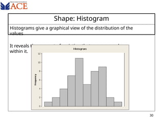
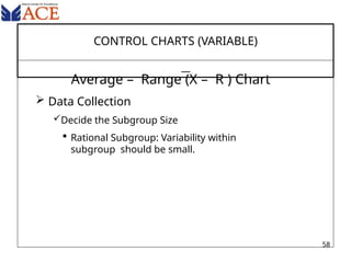
1. By
MARUTI CENTER FOR EXCELLENCE

2. STATISTICAL
PROCESS
CONTROL
SPC
2

3.  Section 1:- SPC Introduction and Concept of Control
Chart
 SPC & Voice of Process
 Variation : Common and Special Cause
 Basic Statistics : Location, Spread, Shape
 Normal Distribution
 Control chart fundamentals
 Type of data and control chart
 Selection of Control charts
 Control chart preparatory steps
 Section 2:- Variable Common Control charts
 X bar & R chart
 Data collection
 Limit calculation and validation
 Process capability – Method of calculation Cp, Cpk, Pp & Ppk
 Control chart interpretation rules
Contents
3

4. Section –
1
4
SPC Introduction and Concept of Control
chart

5. By Definition :- Controlling the process variations by using
statistics is called Statistical Process Control (SPC).
STATISTICS :- Deals with designing for collection of data, data analysis,
interpretation and initiating action based on the analysis .
or
The set of information derived from the Sample data to
estimate the process (Population) are called Statistics.
PROCESS :- Converting an input into an output by using Man,
Machine, Material, Method and Environment.
CONTROL :- Ensuring to make a variable to be with in the stated limit
What is Statistical Process Control
5

6. TRADITIONAL PROCESS CONTROL
PROCESS
Inpu
t
Outpu
t
(Product or Service)
•Based on defect
detection
•Little or no reference to
the process
•A goal post mentality
Inspect
Detec
t
Reject
Correc
t
6

7. Traditional
Philosophy
LSL
7
USL
Anything outside the specification
limits
represents quality losses
Goalpost Mentality

8. PROCESS CONTROL: A BETTER APPROACH
THE PROCESS
Method
Environmen
t People
Equipment
Material
Inpu
t
Outpu
t
(Product or Service)
Collect
Record
Analyze
Act
• Listen Voice of
Process
8

9. Prevention vs. Detection
 In the past, manufacturing depended on inspection
to
screen out nonconforming product
-This process produces rework and scrap, in other words, waste or
lots of MUDA.
-Inspection does not increase quality, it only affects customer
annoyance.
-Detection tolerates waste
 Strategies for prevention are required in today’s
markets
-First, mistake- proof the process
-If mistake- proofing is impractical or impossible, then control the
inputs to prevent nonconforming outputs
-Prevention avoids waste
9

10. VOICE OF THE
PROCESS
THROUGH SPC
10

11. SPC HISTORY
Developed By
Dr.Walter A.
Shewhart
During 1920’s in Bell Lab
Since then SPC has evolved to
cover different
11

12. VARIATION :
The basic principle of SPC
12

13. What is this variation?
• One problem with mother nature, every thing is
different
• No two things can be produced same in this world.
By all efforts we can only reduce the gap between
the two. This gap is known as variation.
• Dissimilarity between two products for the
same characteristic is called variation.
• The inevitable differences among individual outputs
of a process is called variation.
• No two things are exactly alike…
• No two people are same…
• Temperature changes continuously…
• The products we produce change continuously… 13

14. Why do you want to reduce the variation?
• Because variation is the main source of
wastage, undesired reworks, rejections,
customer dissatisfaction and many hidden,
unrecoverable costs.
14

15. Common Causes
• Common to all individual readings in time
periods.
A process operating under common cause is
called
Under statistical control
15

16. Special / Assignable Causes
• Sudden in nature
• Usually attract the attention of local people
associated with the process.
They are not common to all time periods, but they can
cause process fluctuations which are large in
magnitude
16

17. 6.50 6.55 7.00
6.55 a.m. +/- 5 minutes.
This man wants to reach his work place by 6.55 a.m.. But he can
not do so, exactly at 6.55 a.m. daily. Sometimes he reaches earlier
(but almost never before 6.50 a.m.). Sometimes he reaches later
(but almost never after 7.00 a.m.).
WHY ?
17

18. THIS IS BECAUSE....
OF CERTAIN FACTORS WHICH
• Affect the time he takes
• He cannot control
• Vary randomly
– e.g. The traffic you encounter under normal course of
travel
THE VARIATION THAT OCCURS DUE TO THESE KIND
OF FACTORS IS CALLED INHERENT VARIATION
OR COMMON CAUSE VARIATION OR WHITE
NOISE.
– e.g.. m/c vibration,tool wear etc.
18

19. UNDER NORMAL SCHEME OF
OPERATION
Inherent
Variability
(white noise)
Aimed value
Minimum deviation
Maximum deviation
19

20. 6.30
TODAY HE IS EARLY !
WHY ?
PROBABLY BECAUSE :
• His watch was running fast.
• He got a lift.
• His Bus driver took a shortcut.
• He stayed over in the colony.
• He had some important
work to be finished before 7.30.
These causes are characteristic of
a specific circumstance and do
not occur in the normal scheme
of actions.
Variation due to these types of
reasons is called assignable or
special cause variation or black
noise 20

21. 7.20
TODAY HE IS LATE
WHY ?
PROBABLY BECAUSE :
• Heoverslept.
• He missed his Bus.
• The Bus driver was new
• He took some other route
• He stayed over at some
other place.
These causes are characteristic
of a specific circumstance and
do not occur in the normal
scheme of actions.
Variation due to these types of
reasons is called assignable or
special cause variation or
black noise 21

22. GRAPHICAL DISPLAY OF
VARIABILITIES
Inherent
Variability
Assignable
Variability
Assignable
Variability
T
O
T
A
L
V
A
R
I
A
B
I
L
I
T
Y
Assignable
Variability
Assignable
Variability
Aimed Value
CASE I
CASE II
(Black
noise)
22

23. Location
Shape
How to estimate process
behavior ?
Spread
23

24. Process can differ in
;
Locatio
n
24
Sprea
d
Or any
combination
of these
Shape

25. Location : MEAN – Centre of Gravity
estimate
s
The Symbol “Σ” means ‘Sum
of’
N
i N
x
i1
   i

in
n
xi
x 
i1
The Mean of ‘n’ values is the total of the values divided by
‘n’
X 
x1  x2  x3 .....xn
n
In Standard Mathematical Notation it is
25

26. MEAN : Example
Trial Result
1 6
2 3
3 7
4 6
5 10
6 7
7 4
8 8
9 9
10 4
11 8
12 8
13 6
14 7
15 8
Sum 101
mean 6.733
Calculate the mean of the following data
set
26

27. Spread - Range
The difference between the largest and the smallest of a
set of numbers. It is designated by a capital “R”.
54- 45=9
Range is not a very powerful statistic to measure
dispersion
R = Xmax -
Xmin
Examples
R = XHi -
XLow
Data Set 45 47 4
9
51
46 47 4
9
52
47 47 5
0
53
47 48 5
1
54 Range is :
27

28. Spread – Standard Deviation
The average distance between the individual
numbers and the mean. It is designated by “σ”
‘
estimate
s
σ =
(X1-X)2 + (X2-X)2…. (XN-X)2
N
28

29. Determine the standard deviation for the following sample
data set: 1, 2, 3
Standard Deviation : Example
29
S= (-1)2+0+(1)2 =1
2

30. Shape: Histogram
Histograms give a graphical view of the distribution of the
values
It reveals the amount of variation that any process has
within it.
30

31. 31
• A diagram that graphically depicts
the
variability in a population.
WHAT IS HISTOGRAM :

32. 32
• The frequency data obtained from
measurements display a peak around a certain
value. The variation of quality characteristics is
called distribution.
• The figure that illustrates frequency in the form
a pole is referred to as a Histogram.
WHAT IS HISTOGRAM :

33. 33
POPULATION AND SAMPLE
• The entire set of items is called the Population.
• The small number of items taken from the
population to make a judgment of the
population is called a Sample.
• The numbers of samples taken to make this
judgment is called Sample size.
SAMPLE SIZE : THREE
POPULATION

34. Histogram – steps
1.Obtain a set of 50 ~ 100 observations as shown below:
34
Sample
Number
Results of Measurement
1-10 2.510 2.517 2.522 2.522 2.510 2.511 2.519 2.532 2.539 2.525
11-20 2.527 2.536 2.506 2.541 2.512 2.521 2.521 2.536 2.529 2.524
21-30 2.529 2.523 2.523 2.523 2.519 2.538 2.543 2.538 2.518 2.534
31-40 2.520 2.514 2.512 2.534 2.526 2.532 2.532 2.526 2.523 2.520
41-50 2.535 2.523 2.526 2.525 2.532 2.530 2.500 2.530 2.522 2.514
51-60 2.533 2.510 2.542 2.524 2.530 2.535 2.522 2.535 2.540 2.528
61-70 2.525 2.515 2.520 2.519 2.526 2.542 2.522 2.539 2.540 2.528
71-80 2.531 2.545 2.524 2.522 2.520 2.519 2.519 2.529 2.522 2.513
81-90 2.518 2.527 2.511 2.519 2.531 2.527 2.529 2.528 2.519 2.521

35. Histogram – steps
35
2. Obtain the maximum value and minimum value:
Sample
Number
Results of Measurement Maximum
value of the
line
Minimum value of the
line
1-10 2.510 2.5
17
2.5
22
2.5
22
2.5
10
2.5
11
2.5
19
2.5
32
2.5
39
2.5
25
2.539 2.510
11-20 2.527 2.5
36
2.5
06
2.5
41
2.5
12
2.5
21
2.5
21
2.5
36
2.5
29
2.5
24
2.541 2.506
21-30 2.529 2.5
23
2.5
23
2.5
23
2.5
19
2.5
38
2.5
43
2.5
38
2.5
18
2.5
34
2.543 2.518
31-40 2.520 2.5
14
2.5
12
2.5
34
2.5
26
2.5
32
2.5
32
2.5
26
2.5
23
2.5
20
2.534 2.512
41-50 2.535 2.5
23
2.5
26
2.5
25
2.5
32
2.5
30
2.5
00
2.5
30
2.5
22
2.5
14
2.535 2.500
51-60 2.533 2.5
10
2.5
42
2.5
24
2.5
30
2.5
35
2.5
22
2.5
35
2.5
40
2.5
28
2.542 2.510
61-70 2.525 2.5
15
2.5
20
2.5
19
2.5
26
2.5
42
2.5
22
2.5
39
2.5
40
2.5
28
2.539 2.515
71-80 2.531 2.5
45
2.5
24
2.5
22
2.5
20
2.5
19
2.5
19
2.5
29
2.5
22
2.5
13
2.545 2.513
81-90 2.518 2.5
27
2.5
11
2.5
19
2.5
31
2.5
27
2.5
29
2.5
28
2.5
19
2.5
21
2.531 2.511
The largest value
2.545
The smallest value 2.500

36. Table
36
Number of data
(N)
Number of classes
(K)
Unde
r
50 5 - 7
50 - 100 6 - 10
100 - 250 7 - 12
Over 250 10 - 20

37. Histogram- Steps
3. Determine the number of classes:
There are two methods to identify no of class.
1. As per table.
We have data of 90 pcs, which comes under 50-100 range.
We can take 9 class.
2. Second method
 N
 90
 9.48
Therefore, number of interval of classes be taken as 9.
37

38. Histogram- Steps
38
3. Determine width of one class
Range = Max- Min
= 2.545- 2.500
= 0.045
Width of one = Range / No of
class
= 0.045/9
= 0.005
.

39. Class Mid-Point
of Class
x
Frequency Marks (Tally) Freque
ncy f
1 2.500 - 2.505 2.500 / 1
2 2.506 – 2.510 2.508 //// 4
3 2.511 – 2.515 2.513 //// /// 8
4 2.516 – 2.520 2.518 //// //// //// 14
5 2.521 – 2.525 2.523 //// //// //// //// / 21
6 2.526 – 2.530 2.528 //// //// //// // 17
7 2.531 – 2.535 2.533 //// //// // 12
8 2.536 – 2.540 2.538 /////// 8
9 2.541 – 2.545 2.543 //// 5
Total - 90
Histogram –Steps
39
4. Make a frequency table as given below:

40. Histogram-Steps
40
5. Mark the horizontal axis with the
class boundary values.
6. Mark the vertical axis with a
frequency scale.
7. Erect the rectangles over the class
interval having area proportion to
the frequencies.
8 Draw a line on the Histogram to represent
Mean, number of data points and standard
deviation.

41. Histogram
41

42. Histogram
42

43. Normal Distribution
ử±3o
99.7%
ử±2o
95.4%
ử±o
68.3%
ử-3o ử-2o ử-o ử ử+o ử+2o ử+3o
USL
LSL
Out of
Spec.
Out of
Spec.
o
43

44. Histogram for
grade wise distribution
in a class
10
23
35
25
15
5
C- C B B+ A A +
Grade
No.
of
students
44

45. 45
TYPES OF HISTOGRAMS
• Normal
– Bell shaped and natural.
• Comb like
– Regular ups and downs,
– indicates possible measurement error or
rounding problem
• Positive or Negatively skewed
– Possibly due to a limiting process parameter

46. 46
TYPES OF HISTOGRAMS
• Precipice type
– Indicate filtering out through inspection
– Or incorrect representation
• Plateau type
– From multiple sources with small differences in
averages
– Look for stratification
• Bimodal
– Two peaks – coming from two
different sources/populations
• Isolated peak type
i o
n
o
r
– Outliers indicate mistake in sampling, data
collect measurement
– Possibly process shift during data
collection

47. 34.13% 34.13% 13.6%
13.6%
2.14% 2.14%
68.26%
+/- 1 sigma
95.46%
+/- 2 sigma
99.73%
+/-3 sigma
Normal Distribution Curve– Relation between spread & sigma
+ σ
47
+2σ
+3σ
-σ
-2σ
-3σ

48. By collecting sample data from the process
and computing their
 Mean
 Standard deviation and
 Shape
Prediction can be made about the
process
48

49. For routine process control, we
need
•
Simple computation
•
Easy to use by operators for ongoing process control
•
Help the process perform consistently, predictably for quality
and
cost
•
Achieve
Less variation in
output Lower unit
cost
Increase effective
capacity
•
Provide a common
language for
discussing process
performance
49

50. Control Charts
 Transformation of a normal distribution curve in the form of 3 parallel
lines,
where
• The middle line indicates mean and called central line (C.L.)
• The upper line indicates mean Mean +3 Sigma and called upper control limit
(UCL)
• The lower line indicates Mean – 3 Sigma and called lower control limit (LCL)
C.L
50
U.C.L
L.C.L
MEAN
-3σ
+3σ

51. Types of Data
Attribute
Anything that can be
classified Either / Or
Pass / fail
Good /
Bad Go /
No Go
Count
Discrete
Detection
Oriented
51
Variable
Anything that can be
measured Height
Dollars
Distanc
e
Speed
Continuous, infinite
Stimulates
Prevention

52. Common Control Charts
Variable
 Average and Range ( X-R )
 Individual and Moving Range ( X – MR / I –
MR )
Attribute
 p/ np
Chart
 c/ u Chart
: Unit Nonconforming (Defectives)
: Number of Nonconformities
(Defects)
52

53. Steps for Control Charts
1. Complete preparatory
steps
2. Data Collection
3. Making Trial Control
Limits
4. Validation of Control
limits
5. Process Capability Study
6. On going control
7. Improvement
53

54. Control Chart: Preparatory Steps
 Create a suitable (conducive)
environment
 Select characteristics
 Verify Measurement System capability
 Select suitable control chart
54

55. Variable
Data
Rational
Subgroup ?
Ye
s
Subgroup
size >8
X-bar & R Chart
Ye
s
No
Easy To
Compute
Sigma
X-bar & S Chart
Ye
s
No
I & MR Chart
No
% Defective
&
Defects ?
Constant
Sample Size ?
No
% Defective
p-Chart
np-Chart & p-chart
u-Chart
c-Chart & u-chart
No
Ye
s
Constant
Sample Size ?
SPC – Charts For All
Occasions
No
55
Defects
Ye
s
Ye
s

56. Section -
2
56
Variable Common Control Charts

57. CONTROL CHARTS (VARIABLE)
Average – Range (X – R ) Chart
 When ?
Measurement must be variable.
Situation must be practically feasible to have at
least 2
measurements in short span.
Mass Production.
Suitable for Product (Output) Characteristics.
Suitable for both Normal & Non- Normal Data. 57

58. CONTROL CHARTS (VARIABLE)
Average – Range (X – R ) Chart
 Data Collection
Decide the Subgroup Size
 Rational Subgroup: Variability within
subgroup should be small.
58

59. CONTROL CHARTS (VARIABLE)
Average – Range (X – R ) Chart
 Data Collection
Decide Subgroup Frequency
 Detect change in the process over span of time.
 For initial study, may be consecutive or a very
short interval.
59

60. CONTROL CHARTS (VARIABLE)
Average – Range (X – R ) Chart
 Data Collection
Decide no. of subgroups
(For initial study: To Define the control limits)
 To incorporate Major Source of Variation
(Generally 25 subgroups or more Containing
about 100 individual Measurements)
60

61. AVERAGE RANGE CHART
61
CUSTOMER : PART NAME: PART NO.:
PARAMETER: SPEC.(NOMI): 0.70 MACHINE:
TOLERANCE: +/- 0.2
01 02 03 04 05 06 07 08 09 10 11 12 13 14 15 16 17 18 19 20
1 0.65 0.75 0.75 0.60 0.70 0.60 0.7
5
0.60 0.65 0.60 0.80 0.85 0.70 0.65 0.90 0.75 0.75 0.75 0.65 0.60
2 0.70 0.85 0.80 0.70 0.75 0.75 0.7
0
0.70 0.80 0.80 0.70 0.70 0.65 0.60 0.55 0.80 0.65 0.60 0.70 0.85
3 0.65 0.75 0.80 0.70 0.65 0.75 0.6
5
0.80 0.85 0.60 0.90 0.85 0.75 0.85 0.80 0.75 0.85 0.60 0.85 0.65
4 0.65 0.85 0.70 0.75 0.85 0.85 0.6
5
0.65 0.75 0.65 0.70 0.60 0.60 0.65 0.65 0.80 0.60 0.65 0.70 0.70
5 0.85 0.65 0.75 0.65 0.80 0.70 0.8
0
0.75 0.75 0.75 0.65 0.70 0.70 0.60 0.85 0.65 0.80 0.60 0.70 0.65
X
R

62. AVERAGE – RANGE CONTROL CHARTS (X – R )
Calculate Average of each
Subgroup.
Calculate the Range of Each
Subgroup.
R = Xmax – Xmin
 X1 ,X2 ,…. Xn are individual values within the
subgroup
n is the Subgroup Sample Size.
62

63. AVERAGE RANGE CHART
63
CUSTOMER : PART NAME: PART NO.:
PARAMETER: SPEC.(NOMI): 0.70 MACHINE:
TOLERANCE: +/- 0.2
01 02 03 04 05 06 07 08 09 10 11 12 13 14 15 16 17 18 19 20
1 0.65 0.75 0.75 0.60 0.70 0.60 0.75 0.6
0
0.65 0.60 0.80 0.85 0.70 0.65 0.90 0.75 0.75 0.75 0.65 0.60
2 0.70 0.85 0.80 0.70 0.75 0.75 0.70 0.7
0
0.80 0.80 0.70 0.70 0.65 0.60 0.55 0.80 0.65 0.60 0.70 0.85
3 0.65 0.75 0.80 0.70 0.65 0.75 0.65 0.8
0
0.85 0.60 0.90 0.85 0.75 0.85 0.80 0.75 0.85 0.60 0.85 0.65
4 0.65 0.85 0.70 0.75 0.85 0.85 0.65 0.6
5
0.75 0.65 0.70 0.60 0.60 0.65 0.65 0.80 0.60 0.65 0.70 0.70
5 0.85 0.65 0.75 0.65 0.80 0.70 0.80 0.7
5
0.75 0.75 0.65 0.70 0.70 0.60 0.85 0.65 0.80 0.60 0.70 0.65
X 0.70 0.77 0.76 0.68 0.75 0.73 0.71 0.7
0
0.76 0.68 0.75 0.74 0.68 0.67 0.75 0.75 0.73 0.64 0.72 0.69
R 0.20 0.20 0.10 0.15 0.20 0.25 0.15 0.2
0
0.20 0.20 0.25 0.25 0.15 0.25 0.35 0.15 0.25 0.15 0.20 0.25

64. AVERAGE – RANGE CONTROL CHARTS (X – R )
Calculate Average of each
Subgroup.
x 
x1  x2  x3 .....xk
k
Calculate the Average Range.
R 
R1  R2  R3 .....Rk
k
k= No. of subgroups 64

65. AVERAGE – RANGE CONTROL CHARTS (X – R )
Calculate Trial Control Limits for Range
Chart.
Calculate Trial Control Limits for Average
Chart.
D4 , D3 & A2 are Constant varying as per sample size
(n)
65

66. Table of Constants for Control
Charts
n 2 3 4 5 6 7 8 9 10
D4
3.267 2.575 2.282 2.115 2.004 1.924 1.864 1.816 1.777
D3
0 0 0 0 0 0.076 0.136 0.184 0.223
A2
1.880 1.023 0.729 0.577 0.483 0.419 0.373 0.337 0.308
d2
1.128 1.693 2.059 2.326 2.534 2.704 2.847 2.970 3.078
Use the table below where n is the number of samples in a
subgroup.
66

67. AVERAGE – RANGE CONTROL CHARTS (X – R )
x=
0.718
R =
0.21
For R Chart
UCL = D4 X R
LCL = D3 X R
= 0.433
= 0.000
For X Bar Chart
UCL = x + A2 X R = 0.837
LCL = x - A2 X R =
0.5991
67

68. DRAW AVERAGE – RANGE CHART
68

69. A Few Words on Control Limits
Basis for control limits :
•Control limits are also referred to as natural process limits.
•Control limits are based on the mean and standard deviation
of the process as it is, not how we wish it to be.
•There is no connection to specification limits.
Purposes of control limits
•To determine when local action is necessary and to act on it
(i.e., when
special cause variation exists).
•To display the natural variation of the process, that is, the common
cause variation.
•To show any obvious, unnatural patterns in the data.
Specification limits do not belong on control charts.
69

70.  Calculate Process Standard Deviation
σ = R /
d
2
d2 is a constant varying as per sample size (n)
 Calculate Process Capability ( Cp )
Cp = (USL – LSL) / 6σ USL = Upper Specification Limit
LSL = Lower Specification
Limit
= Tolerance / 6σ
Process Capability :
Subgroup Size (n) d2
2 1.128
3 1.693
4 2.059
5 2.326
6 2.534
7 2.704
8 2.847
9 2.970
70

71.  Process spread must be smaller to specification and
 It should be located in a manner that its spread on both
the sides falls well within the specification.
 Capability index that considers both location and spread is
called Cpk
A Problem With Cp
:
-2 -1 0 1 2 3
4
71
-4 -3 -2 -1 0 1 2 3 4 -4
-3
 Cp considers only spread, not the
location.
 For a truly capable process

72. Process Capability Study :
Compare Voice of Process with Voice of
customer (Specification)
Voice of Process
Process Width
USL
LSL
Design Width
Voice of
Customer 72
- 3 σ + 3 σ

73. Calculate Process Capability (Cpk)
Cpu = (USL – X) / 3σ = ZUSL / 3
Or CpL = (X – LSL) / 3σ = ZLSL / 3
Whichever is minimum will be
Cpk
Process Capability :
Subgroup
size(n)
d2
2 1.128
3 1.693
4 2.059
5 2.326
6 2.534
7 2.704
8 2.847
9 2.970
73

74. Standard Deviation (σ) = R / d2
= 0.205 /
2.326
= 0.088
Process Capability :
Cp = (USL-LSL) / 6σ
Cpu = (USL – X) / 3σ
Cpl = (X – LSL) / 3σ
= (0.900-0.500) / 6 X 0.088
= 0.7575
= (0.900-0.718) / 3 X 0.088
= 0.689
= (0.718 – 0.500) / 3 X
0.088
Cpk
Process Capability :
USL = 0.900
LSL = 0.500
X
0.718
USL
(0.900)
74
= 0.8257
= 0.689
LSL
(0.500)

75. Process Capability :
Cp Cpk Remarks
• Process Capable
• Continue Charting
• Bring Cpk closer to Cp
X
• Process has potential Capability
• Improve Cpk by Local action
X X
• Process lacks basic Capability
• Improve process by Management
action
75

76. What about PROCESS PERFORMANCE ?
• Process Capability (Cp, Cpk) indicates the ability of the
process to meet the specification (Voice of customer) when
Process operates under the common causes.
•In practical situation, a process shows variation due to both
common as well as assignable causes.
•One must analyze process behaviour due to combined effect
of Common and Assignable causes. The index is known as
Process Performance Index (Pp, Ppk)
76

77. Process Capability vs Performance :
Cpk Ppk Remarks
• Process Capable and performing
• Continue Charting
X
•Process has Capability but not
performing due to assignable
causes
•Remove assignable causes by
Local action
X X
• Process neither capable nor
performing
• May require Management action 77

78. Other Capability Indices: Machine Capability (Cm, Cmk)
A process variation is
affected by many factors
like
• Raw material variation
• Tools
• Operators
• Measurement System
• Time
• Environmental change
etc…
σ2 Long-Term = σ2 Short-Term
+ σ2 Machines
+ σ2 Day to Day
+ σ2 Operators
+ σ2 Batches
+ σ2 Seasonal
+ ……
Machine capability is an index which is calculated on the basis of
variation contributed by Machine only
78

79. Machine Capability (Cm, Cmk)
• Take 50-100 consecutive samples/ measurements in short
span.
• Ensure the following do not change during
sampling. Raw material batch
Operator
Tooling
Method of process
Measurement
system
Environment etc…
Calculate Cm, Cmk using the same formulae used for Cp, Cpk
79

80. CONTROL CHART: Validation of Control Limit
• Control limits should indicate the variation which
comes due to common causes only. So that, any
assignable assignable cause variation is reflected.
• Hence, it should be based on data when there is
no assignable cause.
• Any control limit based on assignable cause data can
not be considered as Reliable.
•What to do ?
80

81. Validation of Control Limit
10
20
30
40
50
60
0
1 2 3 4 5 6 7 8 9 10 11 12 13 14 15 16 17 18 19 20 21 22 23 24 25
Identify any out of control or special cause situation
 Any point above UCL or below LCL:
R CHART

82. Validation of Control Limits
• For initial control chart,
 Discard all the subgroup showing out of control situation (starting from R-
chart)
 Re-calculate Control Limits, plot and analyse for any out of control
situation.
 Re discard if any out of control situation again found.
 Continue the above cycle until all plot indicate a control situation.
 Repeat same exercise with Average chart.
 If more than 50% data are required to be discarded, reject all data
and re- collect.
 Once initial control chart indicates control situation.
• Calculate Initial Capability
• Extend control limits for ongoing control.
82

83. Control Charts Ongoing Process Control
• Collect the data at the frequency as established.
• Plot on control chart.
• Perform instant analysis and interpretation.
• Give immediate feedback to the process for action if
any
indication of process behaviour change.
•Record significant process events (Tool change, Operator
change,
Shift change, breakdown etc…
•This helps identifying assignable causes.
83

84. Interpreting Control Charts - Ongoing
The interpretation of control charts is based on the statistical
probability of a particular pattern occurring by complete
chance (or being caused by random variation).
• All of the tests identify events that have a less than 0.3%
chance of occurring by random chance (outside of 3s
probability of being caused by random variation).
• Control charts are divided into sigma zones above and
below the average line.
• Zone C is <1 from the mean.
• Zone B is between 1 and 2
• Zone A is between 2 and 3
• Beyond Zone A is > 3
84

85. Control Chart Interpretation
C
B
A
A
B
C
Test 1 The basic test
o Caused by a large change in the
process.
o Requires Immediate action
UCL
LCL
CL
Test:1 One point beyond zone
A
x
x
85

86. Control Chart Interpretation
C
B
A
A
B
C
Test:2 Seven points in a row on one side of center
line.
o Caused by a process mean
shift
LCL
UCL
CL
x
86

87. Control Chart Interpretation
C
B
A
A
B
C
Test:3 Six points in a row steadily increasing or
decreasing
o Caused by
Mechanical wear
Chemical depletion
Increasing
contamination
 etc
LCL
UCL
CL
x
x
87

88. Control Chart Interpretation
C
B
A
A
B
C
Test:4 Alternating Patterns
Fourteen points in a row alternating up &
down
o Caused by
Over adjustment
Shift-to-shift variation
Machine-to-machine
variation
LCL
UCL
CL
x
88

89. Control Chart Interpretation
C
B
A
A
B
C
Test:5 Two out of three points in a row in the same zone A or
beyond
Test 5 The second basic test
o High variation without exceeding the 3 sigma
limit
o Major special cause variation
UCL
LCL
CL
x
x
x
89

90. Control Chart Interpretation
C
B
A
A
B
C
Test:6 Four out of five points in a row in the same zone B and
beyond
o Another test for shift
oTest 1,5,6 are related and show conditions of high special cause
variability.
UCL
LCL
CL
x
x
90

91. Control Chart Interpretation
C
B
A
A
B
C
Test:7 Fifteen points in a row in zone C (Above & below center
line)
Test 7- The Whitespace test
Occurs when within subgroup variation is
large
compared to between group variation or
Old or incorrectly calculated limits
LCL
UCL
CL
x
91

92. Control Chart Interpretation
C
B
A
A
B
C
Test 8 Eight points in a row on both sides of center line with none in
zone C
UCL
LCL
CL
x
Test 8 Alternating Means
Mixtures
Over control
Two different processes on the same
chart.
92

93. Interpretation for Control Charts
93
X Bar Chart R Chart Conclusion
Under Control Under Control Enjoy
Under Control Out of Control Spread Changed
Out of Control Under Control Location Changed
Out of Control Out of Control Both spread and
location changed

94. Individuals (I & MR) Charts
When to use :
Measurement is variable
There is no rational basis for sub grouping or
The measurements are expensive and / or
destructive or
Production rate is slow or
Population is homogeneous
Suitable for both process and product parameters
94

95. Moving Range Control Charts
DATE READING(X) RANGE (R )
1 APR 8.00
2 APR 8.50 0.50
3 APR 7.40 1.10
4 APR 10.50 3.10
5 APR 9.30 1.20
6 APR 11.10 1.80
7 APR 10.40 0.70
8 APR 10.40 0.00
9 APR 9.00 1.40
10 APR 10.00 1.00
11 APR 11.70 1.70
12 APR 10.30 1.40
13 APR 16.20 5.90
14 APR 11.60 4.60
15 APR 11.50 0.10
16 APR 11.00 0.50
17 APR 12.00 1.00
18 APR 11.00 1.00
19 APR 10.20 0.80
20 APR 10.10 0.10
21 APR 10.50 0.40
22 APR 10.30 0.20
23 APR 11.50 1.20
24 APR 11.10 0.40 95

96. Moving Range Control Charts
 Average of Individual
values:
k
x 
x 1
 x 2  x 3  .....x k
x 
8 . 0  8 .5  ...1 1 .1
2 4
x  1 0 .5 7
 Moving Range :
M R 
MR1  MR2  MR3 .....MRk
k 1
M R 
0.5 1.1....0.4
24 1
M R  1.3 96

97. Table of Constants for (I-MR) Charts
Subgroup
Size (n)
d2 D3 D4 E2
2 1.128 - 3.267 2.660
3 1.693 - 2.574 1.772
4 2.059 - 2.282 1.457
5 2.326 - 2.114 1.290
6 2.534 - 2.004 1.184
7 2.704 0.076 1.924 1.109
8 2.847 0.136 1.864 1.054
9 2.970 0.184 1.816 1.010
97

98. Moving Range Control Charts
Upper Control Limits UCLX = X + E2R
UCLX = 10.57 + 2.66*1.3
UCLX = 14.1
Lower Control Limits LCLX = X – E2R
LCLX = 10.57 - 2.66*1.3
LCLX = 7.1
98

99. Moving Range Control Charts
Upper Control Limits UCLR = D4R
UCLR =
3.267*1.3 UCLR =
4.25
Lower Control Limit LCLR = D3R
LCLR = 0*1.3
99

100. Moving Range Control Charts
Upper Control Limits UCLX = 14.1
Lower Control Limits LCLX = 7.1
Upper Control Limits UCLR = 4.3
Lower Control Limit LCLR = 0
Estimate of Standard Deviation of
X :
= 1.3/1.128
=

101. 4.3
0
1.30
2
1
0
6
5
4
3
1 2 3 4 5 6 7 8 9 10 11 12 13 14 15 16 17 18 19 20 21 22 23
Moving Range MR
24
101
Individuals And Range Chart

102. What is Sigma Level (Z-
Score)
• It is a metric, used to quantify how well a
process is performing as compared to
specification.
• It is a measure of the gap between the
specification boundary and Process mean using
σ as a unit of measurement.
• Number of standard deviations that fit between the
average & (upper or lower ) Specification limit.
• A three – sigma level (3
X
LSL USL
σ
102

103. What is Sigma Level (Z-
Score)
• A six – sigma level (6σ)
process
•
LSL X
USL
σ
σ
σ
σ
σ

Sigma Level (USL) 
USL  X
103

104. How to calculate Sigma Level (Z-
Score)

104

or
Sigma Level (LSL) 
Mean  LSL
Sigma Level (USL) 
USL  Mean
Whichever is minimum will be Sigma
level

105. Exampl
e
• Calculate sigma level / Z score / Zigma for the
following data.
LSL = 275, USL = 325, process sigma = 5
and process mean = 305
sigma 5
SigmaLevel 
USL  Mean

325  305
 4
u
sigma 5
Sigma Level 
Mean  LSL

305  275
 6
l
Whichever is
less
Sigma Level = 4
105
Solution
:

106. Sigma Level
Sigma
Level
(Short
Term)
Sigma
Level
(Long
Term)
Defect
opportunity
(Per million)
(Long
Term)
% Yield
(Long Term)
2 0.5 308,770 69.12%
3 1.5 66,811 93.32%
4 2.5 6,210 99.38%
5 3.5 233 99.98%
6 4.5 3.4 99.99966%

107. Normal Distribution
AREA ABOVE z
rea
ab
ove z
0 z
z 0.00 0.01 0.02 0.03 0.04 0.05 0.06 0.07 0.08 0.09
0 0.500000000 0.496010621 0.492021646 0.488033473 0.484046501 0.480061127 0.476077747 0.472096760 0.468118560 0.464143544
0.1 0.460172104 0.456204636 0.452241530 0.448283177 0.444329967 0.440382288 0.436440527 0.432505067 0.428576291 0.424654580
0.2 0.420740313 0.416833866 0.412935613 0.409045927 0.405165176 0.401293726 0.397431943 0.393580186 0.389738814 0.385908182
0.3 0.382088643 0.378280543 0.374484230 0.370700045 0.366928327 0.363169410 0.359423626 0.355691301 0.351972760 0.348268323
0.4 0.344578303 0.340903014 0.337242763 0.333597852 0.329968580 0.326355241 0.322758126 0.319177519 0.315613701 0.312066949
0.5 0.308537533 0.305025719 0.301531771 0.298055944 0.294598489 0.291159655 0.287739682 0.284338808 0.280957264 0.277595276
0.6 0.274253065 0.270930848 0.267628834 0.264347230 0.261086235 0.257846044 0.254626846 0.251428824 0.248252158 0.245097021
0.7 0.241963578 0.238851994 0.235762424 0.232695018 0.229649924 0.226627280 0.223627221 0.220649876 0.217695369 0.214763817
0.8 0.211855334 0.208970026 0.206107994 0.203269335 0.200454139 0.197662492 0.194894473 0.192150158 0.189429614 0.186732906
0.9 0.184060092 0.181411225 0.178786354 0.176185520 0.173608762 0.171056112 0.168527597 0.166023240 0.163543057 0.161087061
1 0.158655260 0.156247655 0.153864244 0.151505020 0.149169971 0.146859081 0.144572328 0.142309686 0.140071125 0.137856610
1.1 0.135666102 0.133499557 0.131356927 0.129238161 0.127143201 0.125071989 0.123024458 0.121000541 0.119000166 0.117023256
1.2 0.115069732 0.113139509 0.111232501 0.109348617 0.107487762 0.105649839 0.103834747 0.102042381 0.100272634 0.098525394
1.3 0.096800549 0.095097982 0.093417573 0.091759198 0.090122734 0.088508052 0.086915021 0.085343508 0.083793378 0.082264493
1.4 0.080756711 0.079269891 0.077803888 0.076358555 0.074933743 0.073529300 0.072145075 0.070780913 0.069436656 0.068112148
1.5 0.066807229 0.065521737 0.064255510 0.063008383 0.061780193 0.060570771 0.059379950 0.058207562 0.057053437 0.055917403
1.6 0.054799289 0.053698923 0.052616130 0.051550737 0.050502569 0.049471451 0.048457206 0.047459659 0.046478632 0.045513949
1.7 0.044565432 0.043632903 0.042716185 0.041815099 0.040929468 0.040059114 0.039203858 0.038363523 0.037537931 0.036726904
1.8 0.035930266 0.035147838 0.034379445 0.033624911 0.032884058 0.032156713 0.031442700 0.030741845 0.030053974 0.029378914
1.9 0.028716493 0.028066539 0.027428881 0.026803350 0.026189776 0.025587990 0.024997825 0.024419115 0.023851694 0.023295398
2 0.022750062 0.022215525 0.021691624 0.021178201 0.020675095 0.020182148 0.019699203 0.019226106 0.018762701 0.018308836
2.1 0.017864357 0.017429116 0.017002962 0.016585747 0.016177325 0.015777551 0.015386280 0.015003369 0.014628679 0.014262068
2.2 0.013903399 0.013552534 0.013209339 0.012873678 0.012545420 0.012224433 0.011910588 0.011603756 0.011303811 0.011010627
2.3 0.010724081 0.010444050 0.010170414 0.009903053 0.009641850 0.009386687 0.009137452 0.008894029 0.008656308 0.008424177
2.4 0.008197529 0.007976255 0.007760251 0.007549411 0.007343633 0.007142815 0.006946857 0.006755661 0.006569129 0.006387167
2.5 0.006209680 0.006036575 0.005867760 0.005703147 0.005542646 0.005386170 0.005233635 0.005084954 0.004940046 0.004798829
2.6 0.004661222 0.004527147 0.004396526 0.004269282 0.004145342 0.004024631 0.003907076 0.003792607 0.003681155 0.003572649
2.7 0.003467023 0.003364211 0.003264148 0.003166769 0.003072013 0.002979819 0.002890125 0.002802872 0.002718003 0.002635461
2.8 0.002555191 0.002477136 0.002401244 0.002327463 0.002255740 0.002186026 0.002118270 0.002052424 0.001988442 0.001926276
2.9 0.001865880 0.001807211 0.001750225 0.001694878 0.001641129 0.001588938 0.001538264 0.001489068 0.001441311 0.001394956
3 0.001349967 0.001306308 0.001263943 0.001222838 0.001182960 0.001144276 0.001106754 0.001070363 0.001035071 0.0011000078
51

108. z 0.00 0.01 0.02 0.03 0.04 0.05 0.06 0.07 0.08 0.09
3.1 0.000967671 0.000935504 0.000904323 0.000874099 0.000844806 0.000816419 0.000788912 0.000762260 0.000736440 0.000711429
3.2 0.000687202 0.000663738 0.000641016 0.000619014 0.000597711 0.000577086 0.000557122 0.000537798 0.000519095 0.000500996
3.3 0.000483483 0.000466538 0.000450144 0.000434286 0.000418948 0.000404113 0.000389767 0.000375895 0.000362482 0.000349515
3.4 0.000336981 0.000324865 0.000313156 0.000301840 0.000290906 0.000280341 0.000270135 0.000260276 0.000250753 0.000241555
3.5 0.000232673 0.000224097 0.000215816 0.000207822 0.000200105 0.000192656 0.000185467 0.000178530 0.000171836 0.000165377
3.6 0.000159146 0.000153135 0.000147337 0.000141746 0.000136353 0.000131154 0.000126141 0.000121308 0.000116649 0.000112158
3.7 0.000107830 0.000103659 0.000099641 0.000095768 0.000092038 0.000088445 0.000084983 0.000081650 0.000078440 0.000075349
3.8 0.000072372 0.000069507 0.000066749 0.000064094 0.000061539 0.000059081 0.000056715 0.000054438 0.000052248 0.000050142
3.9 0.000048116 0.000046167 0.000044293 0.000042491 0.000040758 0.000039092 0.000037491 0.000035952 0.000034473 0.000033052
4 0.000031686 0.000030374 0.000029113 0.000027902 0.000026739 0.000025622 0.000024549 0.000023519 0.000022530 0.000021580
4.1 0.000020669 0.000019794 0.000018954 0.000018148 0.000017375 0.000016633 0.000015922 0.000015239 0.000014584 0.000013956
4.2 0.000013354 0.000012777 0.000012223 0.000011692 0.000011183 0.000010696 0.000010228 0.000009780 0.000009351 0.000008940
4.3 0.000008546 0.000008169 0.000007807 0.000007461 0.000007130 0.000006812 0.000006508 0.000006217 0.000005939 0.000005672
4.4 0.000005417 0.000005173 0.000004939 0.000004716 0.000004502 0.000004297 0.000004102 0.000003914 0.000003736 0.000003564
4.5 0.000003401 0.000003244 0.000003095 0.000002952 0.000002815 0.000002685 0.000002560 0.000002441 0.000002327 0.000002218
4.6 0.000002115 0.000002015 0.000001921 0.000001830 0.000001744 0.000001661 0.000001583 0.000001508 0.000001436 0.000001368
4.7 0.000001302 0.000001240 0.000001181 0.000001124 0.000001070 0.000001018 0.000000969 0.000000922 0.000000878 0.000000835
4.8 0.000000794 0.000000756 0.000000719 0.000000684 0.000000650 0.000000618 0.000000588 0.000000559 0.000000531 0.000000505
4.9 0.000000480 0.000000456 0.000000433 0.000000412 0.000000391 0.000000372 0.000000353 0.000000335 0.000000318 0.000000302
5 0.000000287 0.000000273 0.000000259 0.000000246 0.000000233 0.000000221 0.000000210 0.000000199 0.000000189 0.000000179
5.1 0.000000170 0.000000161 0.000000153 0.000000145 0.000000138 0.000000130 0.000000124 0.000000117 0.000000111 0.000000105
5.2 0.000000100 0.000000095 0.000000090 0.000000085 0.000000080 0.000000076 0.000000072 0.000000068 0.000000065 0.000000061
5.3 0.000000058 0.000000055 0.000000052 0.000000049 0.000000047 0.000000044 0.000000042 0.000000039 0.000000037 0.000000035
5.4 0.000000033 0.000000032 0.000000030 0.000000028 0.000000027 0.000000025 0.000000024 0.000000023 0.000000021 0.000000020
5.5 0.000000019 0.000000018 0.000000017 0.000000016 0.000000015 0.000000014 0.000000014 0.000000013 0.000000012 0.000000011
5.6 0.000000011 0.000000010 0.000000010 0.000000009 0.000000009 0.000000008 0.000000008 0.000000007 0.000000007 0.000000006
5.7 0.000000006 0.000000006 0.000000005 0.000000005 0.000000005 0.000000004 0.000000004 0.000000004 0.000000004 0.000000004
5.8 0.000000003 0.000000003 0.000000003 0.000000003 0.000000003 0.000000002 0.000000002 0.000000002 0.000000002 0.000000002
5.9 0.000000002 0.000000002 0.000000002 0.000000002 0.000000001 0.000000001 0.000000001 0.000000001 0.000000001 0.000000001
6 0.000000001 0.000000001 0.000000001 0.000000001 0.000000001 0.000000001 0.000000001 0.000000001 0.000000001 0.000000001
7 0.000000000
8 0.000000000
9 0.000000000
10 0.000000000
108

109. Glossary of
Terms
Process capability is determined by the
variation that comes from common causes. It
generally represents the best performance of
the process itself. This is demonstrated when
the process is being operated in a state of
statistical control regardless of the
specifications.
Process Capability – The 6 σ range of
inherent process variation, for statistically
stable processes only, where σ is usually
estimated by
109

110. Customers, internal or external, are however
more typically concerned with the process
performance ; that is, the overall output of the
process and how it relates to their
requirements (defined by specifications),
irrespective of the process variation.
Process Performance - The 6 range of total
process variation, where σ is usually estimated
by s, the total process standard deviation.
n
110

i
i
x  x 2
n 1
 p  S


111. Range : A measure of process spread. The
difference between the highest and lowest
values in a subgroup, a sample, or a
population.
Variable Data : Quantitative data, where
measurements are used for analysis. Examples
include the diameter of a bearing in
millimeters, the closing effort of a door in
Newtons, torque of a fastener in Newton-
meters.
Attributes Data : Qualitative data that can be
categorized for recording and analysis.
Examples : where the results are recorded in a
simple yes/no fashion, such as acceptability of111

112. THANK YOU