a

1. © 2008 Prentice Hall, Inc. S6 – 1
Statistical Process Control
Statistical Process Control

2. © 2008 Prentice Hall, Inc. S6 – 2
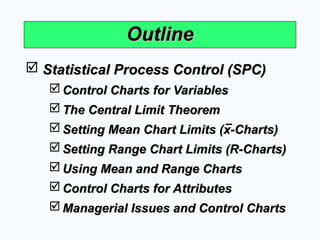
Outline
Outline
 Statistical Process Control (SPC)
Statistical Process Control (SPC)
 Control Charts for Variables
Control Charts for Variables
 The Central Limit Theorem
The Central Limit Theorem
 Setting Mean Chart Limits (x-Charts)
Setting Mean Chart Limits (x-Charts)
 Setting Range Chart Limits (R-Charts)
Setting Range Chart Limits (R-Charts)
 Using Mean and Range Charts
Using Mean and Range Charts
 Control Charts for Attributes
Control Charts for Attributes
 Managerial Issues and Control Charts
Managerial Issues and Control Charts

3. © 2008 Prentice Hall, Inc. S6 – 3
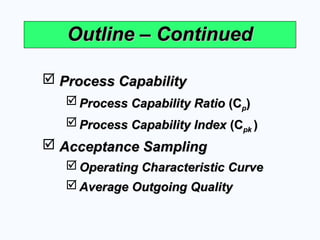
Outline – Continued
Outline – Continued
 Process Capability
Process Capability
 Process Capability Ratio
Process Capability Ratio (C
(Cp
p)
)
 Process Capability Index
Process Capability Index (C
(Cpk
pk )
)
 Acceptance Sampling
Acceptance Sampling
 Operating Characteristic Curve
Operating Characteristic Curve
 Average Outgoing Quality
Average Outgoing Quality

4. © 2008 Prentice Hall, Inc. S6 – 4
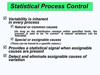
 Variability is inherent
Variability is inherent
in every process
in every process
 Natural or common causes
Natural or common causes
(As long as the distribution remains within specified limits, the
(As long as the distribution remains within specified limits, the
process is said to be “in control” & natural variations can be
process is said to be “in control” & natural variations can be
tolerated)
tolerated)
 Special or assignable causes
Special or assignable causes
(These can be traced to a specific reason.)
(These can be traced to a specific reason.)
 Provides a statistical signal when assignable
Provides a statistical signal when assignable
causes are present
causes are present
 Detect and eliminate assignable causes of
Detect and eliminate assignable causes of
variation
variation
Statistical Process Control
Statistical Process Control

5. © 2008 Prentice Hall, Inc. S6 – 5
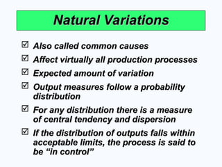
Natural Variations
Natural Variations
 Also called common causes
Also called common causes
 Affect virtually all production processes
Affect virtually all production processes
 Expected amount of variation
Expected amount of variation
 Output measures follow a probability
Output measures follow a probability
distribution
distribution
 For any distribution there is a measure
For any distribution there is a measure
of central tendency and dispersion
of central tendency and dispersion
 If the distribution of outputs falls within
If the distribution of outputs falls within
acceptable limits, the process is said to
acceptable limits, the process is said to
be “in control”
be “in control”

6. © 2008 Prentice Hall, Inc. S6 – 6
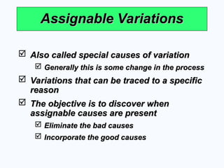
Assignable Variations
Assignable Variations
 Also called special causes of variation
Also called special causes of variation
 Generally this is some change in the process
Generally this is some change in the process
 Variations that can be traced to a specific
Variations that can be traced to a specific
reason
reason
 The objective is to discover when
The objective is to discover when
assignable causes are present
assignable causes are present
 Eliminate the bad causes
Eliminate the bad causes
 Incorporate the good causes
Incorporate the good causes

7. © 2008 Prentice Hall, Inc. S6 – 7
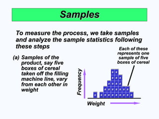
Samples
Samples
To measure the process, we take samples
To measure the process, we take samples
and analyze the sample statistics following
and analyze the sample statistics following
these steps
these steps
(a)
(a) Samples of the
Samples of the
product, say five
product, say five
boxes of cereal
boxes of cereal
taken off the filling
taken off the filling
machine line, vary
machine line, vary
from each other in
from each other in
weight
weight
Frequency
Frequency
Weight
Weight
#
#
#
#
#
# #
#
#
#
#
#
#
#
#
#
#
#
#
# #
# #
#
#
# #
# #
#
#
#
#
# #
# #
#
#
# #
# #
#
#
# #
# #
#
#
#
Each of these
Each of these
represents one
represents one
sample of five
sample of five
boxes of cereal
boxes of cereal

8. © 2008 Prentice Hall, Inc. S6 – 8
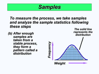
Samples
Samples
To measure the process, we take samples
To measure the process, we take samples
and analyze the sample statistics following
and analyze the sample statistics following
these steps
these steps
(b)
(b) After enough
After enough
samples are
samples are
taken from a
taken from a
stable process,
stable process,
they form a
they form a
pattern called a
pattern called a
distribution
distribution
The solid line
The solid line
represents the
represents the
distribution
distribution
Frequency
Frequency
Weight
Weight

9. © 2008 Prentice Hall, Inc. S6 – 9
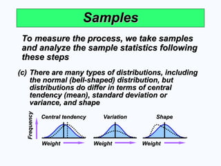
Samples
Samples
To measure the process, we take samples
To measure the process, we take samples
and analyze the sample statistics following
and analyze the sample statistics following
these steps
these steps
(c)
(c) There are many types of distributions, including
There are many types of distributions, including
the normal (bell-shaped) distribution, but
the normal (bell-shaped) distribution, but
distributions do differ in terms of central
distributions do differ in terms of central
tendency (mean), standard deviation or
tendency (mean), standard deviation or
variance, and shape
variance, and shape
Weight
Weight
Central tendency
Central tendency
Weight
Weight
Variation
Variation
Weight
Weight
Shape
Shape
Frequency
Frequency

10. © 2008 Prentice Hall, Inc. S6 – 10
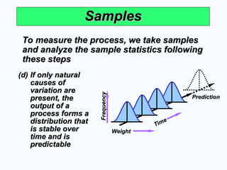
Samples
Samples
To measure the process, we take samples
To measure the process, we take samples
and analyze the sample statistics following
and analyze the sample statistics following
these steps
these steps
(d)
(d) If only natural
If only natural
causes of
causes of
variation are
variation are
present, the
present, the
output of a
output of a
process forms a
process forms a
distribution that
distribution that
is stable over
is stable over
time and is
time and is
predictable
predictable
Weight
Weight
Time
Time
Frequency
Frequency
Prediction
Prediction

11. © 2008 Prentice Hall, Inc. S6 – 11
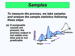
Samples
Samples
To measure the process, we take samples
To measure the process, we take samples
and analyze the sample statistics following
and analyze the sample statistics following
these steps
these steps
(e)
(e) If assignable
If assignable
causes are
causes are
present, the
present, the
process output is
process output is
not stable over
not stable over
time and is not
time and is not
predicable
predicable
Weight
Weight
Time
Time
Frequency
Frequency
Prediction
Prediction
?
?
?
?
?
?
?
?
?
?
?
?
?
?
?
?
?
?
?
?
?
?
?
?
?
?
?
?
?
?
?
?
?
?
?
??
?

12. © 2008 Prentice Hall, Inc. S6 – 12
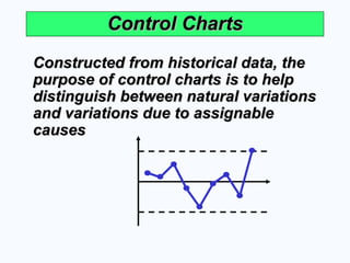
Control Charts
Control Charts
Constructed from historical data, the
Constructed from historical data, the
purpose of control charts is to help
purpose of control charts is to help
distinguish between natural variations
distinguish between natural variations
and variations due to assignable
and variations due to assignable
causes
causes

13. © 2008 Prentice Hall, Inc. S6 – 13
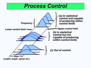
Process Control
Process Control
Frequency
Frequency
(weight, length, speed, etc.)
(weight, length, speed, etc.)
Size
Size
Lower control limit
Lower control limit Upper control limit
Upper control limit
(a) In statistical
(a) In statistical
control and capable
control and capable
of producing within
of producing within
control limits
control limits
(b) In statistical
(b) In statistical
control but not
control but not
capable of producing
capable of producing
within control limits
within control limits
(c) Out of control
(c) Out of control

14. © 2008 Prentice Hall, Inc. S6 – 14
Types of Data
Types of Data
 Characteristics that
Characteristics that
can take any real
can take any real
value
value
 May be in whole or
May be in whole or
in fractional
in fractional
numbers
numbers
 Continuous random
Continuous random
variables
variables
Variables
Variables Attributes
Attributes
 Defect-related
Defect-related
characteristics
characteristics
 Classify products
Classify products
as either good or
as either good or
bad or count
bad or count
defects
defects
 Categorical or
Categorical or
discrete random
discrete random
variables
variables

15. © 2008 Prentice Hall, Inc. S6 – 15
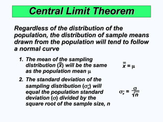
Central Limit Theorem
Central Limit Theorem
Regardless of the distribution of the
Regardless of the distribution of the
population, the distribution of sample means
population, the distribution of sample means
drawn from the population will tend to follow
drawn from the population will tend to follow
a normal curve
a normal curve
1.
1. The mean of the sampling
The mean of the sampling
distribution
distribution (
(x
x)
) will be the same
will be the same
as the population mean
as the population mean 

x =
x = 



n
n

x
x =
=
2.
2. The standard deviation of the
The standard deviation of the
sampling distribution
sampling distribution (
(
x
x)
) will
will
equal the population standard
equal the population standard
deviation
deviation (
(
)
) divided by the
divided by the
square root of the sample size, n
square root of the sample size, n

16. © 2008 Prentice Hall, Inc. S6 – 16
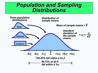
Population and Sampling
Population and Sampling
Distributions
Distributions
Three population
Three population
distributions
distributions
Beta
Normal
Uniform
Distribution of
Distribution of
sample means
sample means
Standard
Standard
deviation of
deviation of
the sample
the sample
means
means
=
= 
x
x =
=


n
n
Mean of sample means = x
Mean of sample means = x
| | | | | | |
-
-3
3
x
x -
-2
2
x
x -
-1
1
x
x x
x +
+1
1
x
x +
+2
2
x
x +
+3
3
x
x
99.73%
99.73% of all x
of all x
fall within
fall within ± 3
± 3
x
x
95.45%
95.45% fall within
fall within ± 2
± 2
x
x

17. © 2008 Prentice Hall, Inc. S6 – 17
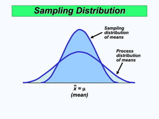
Sampling Distribution
Sampling Distribution
x =
x = 

(mean)
(mean)
Sampling
Sampling
distribution
distribution
of means
of means
Process
Process
distribution
distribution
of means
of means

18. © 2008 Prentice Hall, Inc. S6 – 18
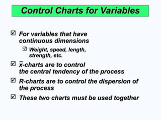
Control Charts for Variables
Control Charts for Variables
 For variables that have
For variables that have
continuous dimensions
continuous dimensions
 Weight, speed, length,
Weight, speed, length,
strength, etc.
strength, etc.
 x-charts are to control
x-charts are to control
the central tendency of the process
the central tendency of the process
 R-charts are to control the dispersion of
R-charts are to control the dispersion of
the process
the process
 These two charts must be used together
These two charts must be used together

19. © 2008 Prentice Hall, Inc. S6 – 19
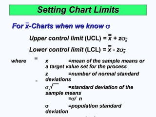
Setting Chart Limits
Setting Chart Limits
For x-Charts when we know
For x-Charts when we know 

Upper control limit
Upper control limit (UCL)
(UCL) = x + z
= x + z
x
x
Lower control limit
Lower control limit (LCL)
(LCL) = x - z
= x - z
x
x
where
where x
x =
=mean of the sample means or
mean of the sample means or
a target value set for the process
a target value set for the process
z
z =
=number of normal standard
number of normal standard
deviations
deviations

x
x =
=standard deviation of the
standard deviation of the
sample means
sample means
=
=
/ n
/ n

 =
=population standard
population standard
deviation
deviation

20. © 2008 Prentice Hall, Inc. S6 – 20
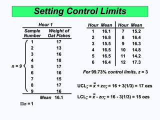
Setting Control Limits
Setting Control Limits
Hour 1
Hour 1
Sample
Sample Weight of
Weight of
Number
Number Oat Flakes
Oat Flakes
1
1 17
17
2
2 13
13
3
3 16
16
4
4 18
18
5
5 17
17
6
6 16
16
7
7 15
15
8
8 17
17
9
9 16
16
Mean
Mean 16.1
16.1

 =
= 1
1
Hour
Hour Mean
Mean Hour
Hour Mean
Mean
1
1 16.1
16.1 7
7 15.2
15.2
2
2 16.8
16.8 8
8 16.4
16.4
3
3 15.5
15.5 9
9 16.3
16.3
4
4 16.5
16.5 10
10 14.8
14.8
5
5 16.5
16.5 11
11 14.2
14.2
6
6 16.4
16.4 12
12 17.3
17.3
n = 9
n = 9
LCL
LCLx
x = x - z
= x - z
x
x =
= 16 - 3(1/3) = 15 ozs
16 - 3(1/3) = 15 ozs
For
For 99.73%
99.73% control limits, z
control limits, z = 3
= 3
UCL
UCLx
x = x + z
= x + z
x
x = 16 + 3(1/3) = 17 ozs
= 16 + 3(1/3) = 17 ozs

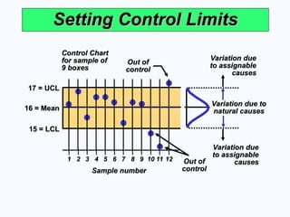
21. © 2008 Prentice Hall, Inc. S6 – 21
Setting Control Limits
Setting Control Limits
17 = UCL
17 = UCL
15 = LCL
15 = LCL
16 = Mean
16 = Mean
Control Chart
Control Chart
for sample of
for sample of
9 boxes
9 boxes
Sample number
Sample number
|
| |
| |
| |
| |
| |
| |
| |
| |
| |
| |
| |
|
1
1 2
2 3
3 4
4 5
5 6
6 7
7 8
8 9
9 10
10 11
11 12
12
Variation due
Variation due
to assignable
to assignable
causes
causes
Variation due
Variation due
to assignable
to assignable
causes
causes
Variation due to
Variation due to
natural causes
natural causes
Out of
Out of
control
control
Out of
Out of
control
control

22. © 2008 Prentice Hall, Inc. S6 – 22
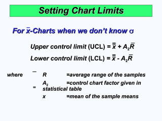
Setting Chart Limits
Setting Chart Limits
For x-Charts when we don’t know
For x-Charts when we don’t know 

Lower control limit
Lower control limit (LCL)
(LCL) = x - A
= x - A2
2R
R
Upper control limit
Upper control limit (UCL)
(UCL) = x + A
= x + A2
2R
R
where
where R
R =
=average range of the samples
average range of the samples
A
A2
2 =
=control chart factor given in
control chart factor given in
statistical table
statistical table
x
x =
=mean of the sample means
mean of the sample means

23. © 2008 Prentice Hall, Inc. S6 – 23
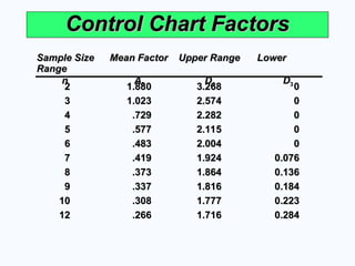
Control Chart Factors
Control Chart Factors
Sample Size
Sample Size Mean Factor
Mean Factor Upper Range
Upper Range Lower
Lower
Range
Range
n
n A
A2
2 D
D4
4 D
D3
3
2
2 1.880
1.880 3.268
3.268 0
0
3
3 1.023
1.023 2.574
2.574 0
0
4
4 .729
.729 2.282
2.282 0
0
5
5 .577
.577 2.115
2.115 0
0
6
6 .483
.483 2.004
2.004 0
0
7
7 .419
.419 1.924
1.924 0.076
0.076
8
8 .373
.373 1.864
1.864 0.136
0.136
9
9 .337
.337 1.816
1.816 0.184
0.184
10
10 .308
.308 1.777
1.777 0.223
0.223
12
12 .266
.266 1.716
1.716 0.284
0.284

24. © 2008 Prentice Hall, Inc. S6 – 24
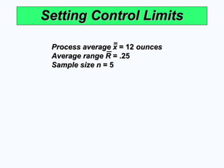
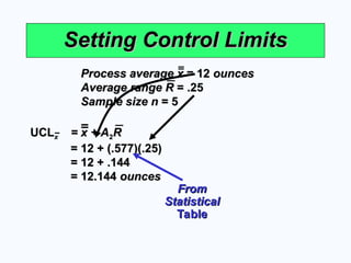
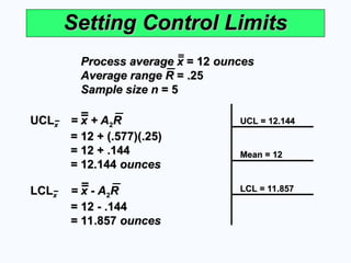
Setting Control Limits
Setting Control Limits
Process average x
Process average x = 12
= 12 ounces
ounces
Average range R
Average range R = .25
= .25
Sample size n
Sample size n = 5
= 5

25. © 2008 Prentice Hall, Inc. S6 – 25
Setting Control Limits
Setting Control Limits
UCL
UCLx
x = x + A
= x + A2
2R
R
= 12 + (.577)(.25)
= 12 + (.577)(.25)
= 12 + .144
= 12 + .144
= 12.144
= 12.144 ounces
ounces
Process average x
Process average x = 12
= 12 ounces
ounces
Average range R
Average range R = .25
= .25
Sample size n
Sample size n = 5
= 5
From
From
Statistical
Statistical
Table
Table

26. © 2008 Prentice Hall, Inc. S6 – 26
Setting Control Limits
Setting Control Limits
UCL
UCLx
x = x + A
= x + A2
2R
R
= 12 + (.577)(.25)
= 12 + (.577)(.25)
= 12 + .144
= 12 + .144
= 12.144
= 12.144 ounces
ounces
LCL
LCLx
x = x - A
= x - A2
2R
R
= 12 - .144
= 12 - .144
= 11.857
= 11.857 ounces
ounces
Process average x
Process average x = 12
= 12 ounces
ounces
Average range R
Average range R = .25
= .25
Sample size n
Sample size n = 5
= 5
UCL = 12.144
UCL = 12.144
Mean = 12
Mean = 12
LCL = 11.857
LCL = 11.857

27. © 2008 Prentice Hall, Inc. S6 – 27
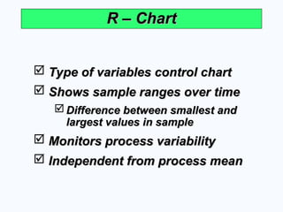
R – Chart
R – Chart
 Type of variables control chart
Type of variables control chart
 Shows sample ranges over time
Shows sample ranges over time
 Difference between smallest and
Difference between smallest and
largest values in sample
largest values in sample
 Monitors process variability
Monitors process variability
 Independent from process mean
Independent from process mean

28. © 2008 Prentice Hall, Inc. S6 – 28
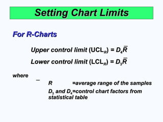
Setting Chart Limits
Setting Chart Limits
For R-Charts
For R-Charts
Lower control limit
Lower control limit (LCL
(LCLR
R)
) = D
= D3
3R
R
Upper control limit
Upper control limit (UCL
(UCLR
R)
) = D
= D4
4R
R
where
where
R
R =
=average range of the samples
average range of the samples
D
D3
3 and D
and D4
4=
=control chart factors from
control chart factors from
statistical table
statistical table

29. © 2008 Prentice Hall, Inc. S6 – 29
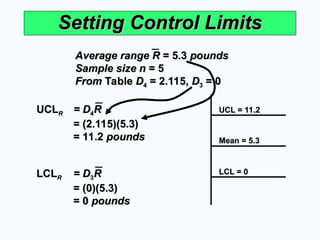
Setting Control Limits
Setting Control Limits
UCL
UCLR
R = D
= D4
4R
R
= (2.115)(5.3)
= (2.115)(5.3)
= 11.2
= 11.2 pounds
pounds
LCL
LCLR
R = D
= D3
3R
R
= (0)(5.3)
= (0)(5.3)
= 0
= 0 pounds
pounds
Average range R
Average range R = 5.3
= 5.3 pounds
pounds
Sample size n
Sample size n = 5
= 5
From
From Table
Table D
D4
4 = 2.115,
= 2.115, D
D3
3 = 0
= 0
UCL = 11.2
UCL = 11.2
Mean = 5.3
Mean = 5.3
LCL = 0
LCL = 0

30. © 2008 Prentice Hall, Inc. S6 – 30
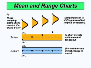
Mean and Range Charts
Mean and Range Charts
(a)
(a)
These
These
sampling
sampling
distributions
distributions
result in the
result in the
charts below
charts below
(Sampling mean is
(Sampling mean is
shifting upward but
shifting upward but
range is consistent)
range is consistent)
R-chart
R-chart
(R-chart does not
(R-chart does not
detect change in
detect change in
mean)
mean)
UCL
UCL
LCL
LCL
x-chart
x-chart
(x-chart detects
(x-chart detects
shift in central
shift in central
tendency)
tendency)
UCL
UCL
LCL
LCL

31. © 2008 Prentice Hall, Inc. S6 – 31
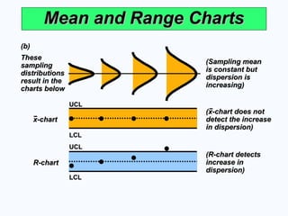
Mean and Range Charts
Mean and Range Charts
R-chart
R-chart
(R-chart detects
(R-chart detects
increase in
increase in
dispersion)
dispersion)
UCL
UCL
LCL
LCL
(b)
(b)
These
These
sampling
sampling
distributions
distributions
result in the
result in the
charts below
charts below
(Sampling mean
(Sampling mean
is constant but
is constant but
dispersion is
dispersion is
increasing)
increasing)
x-chart
x-chart
(x-chart does not
(x-chart does not
detect the increase
detect the increase
in dispersion)
in dispersion)
UCL
UCL
LCL
LCL

32. © 2008 Prentice Hall, Inc. S6 – 32
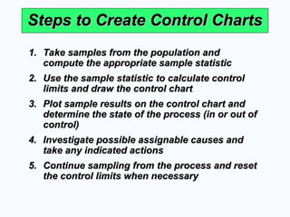
Steps to Create Control Charts
Steps to Create Control Charts
1.
1. Take samples from the population and
Take samples from the population and
compute the appropriate sample statistic
compute the appropriate sample statistic
2.
2. Use the sample statistic to calculate control
Use the sample statistic to calculate control
limits and draw the control chart
limits and draw the control chart
3.
3. Plot sample results on the control chart and
Plot sample results on the control chart and
determine the state of the process (in or out of
determine the state of the process (in or out of
control)
control)
4.
4. Investigate possible assignable causes and
Investigate possible assignable causes and
take any indicated actions
take any indicated actions
5.
5. Continue sampling from the process and reset
Continue sampling from the process and reset
the control limits when necessary
the control limits when necessary

33. © 2008 Prentice Hall, Inc. S6 – 33
Manual and Automated
Manual and Automated
Control Charts
Control Charts

34. © 2008 Prentice Hall, Inc. S6 – 34
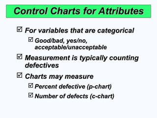
Control Charts for Attributes
Control Charts for Attributes
 For variables that are categorical
For variables that are categorical
 Good/bad, yes/no,
Good/bad, yes/no,
acceptable/unacceptable
acceptable/unacceptable
 Measurement is typically counting
Measurement is typically counting
defectives
defectives
 Charts may measure
Charts may measure
 Percent defective (p-chart)
Percent defective (p-chart)
 Number of defects (c-chart)
Number of defects (c-chart)

35. © 2008 Prentice Hall, Inc. S6 – 35
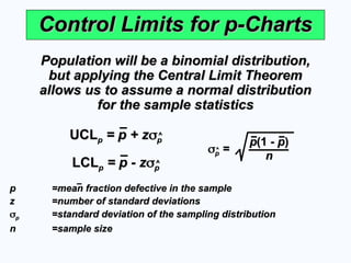
Control Limits for p-Charts
Control Limits for p-Charts
Population will be a binomial distribution,
Population will be a binomial distribution,
but applying the Central Limit Theorem
but applying the Central Limit Theorem
allows us to assume a normal distribution
allows us to assume a normal distribution
for the sample statistics
for the sample statistics
UCL
UCLp
p = p + z
= p + z
p
p
^
^
LCL
LCLp
p = p - z
= p - z
p
p
^
^
p
p =
=mean fraction defective in the sample
mean fraction defective in the sample
z
z =
=number of standard deviations
number of standard deviations

p
p =
=standard deviation of the sampling distribution
standard deviation of the sampling distribution
n
n =
=sample size
sample size
^
^
p
p(1 -
(1 - p
p)
)
n
n

p
p =
=
^
^

36. © 2008 Prentice Hall, Inc. S6 – 36
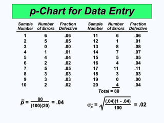
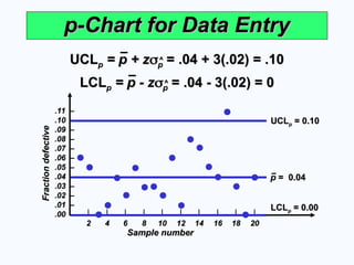
p-Chart for Data Entry
p-Chart for Data Entry
Sample
Sample Number
Number Fraction
Fraction Sample
Sample Number
Number Fraction
Fraction
Number
Number of Errors
of Errors Defective
Defective Number
Number of Errors
of Errors Defective
Defective
1
1 6
6 .06
.06 11
11 6
6 .06
.06
2
2 5
5 .05
.05 12
12 1
1 .01
.01
3
3 0
0 .00
.00 13
13 8
8 .08
.08
4
4 1
1 .01
.01 14
14 7
7 .07
.07
5
5 4
4 .04
.04 15
15 5
5 .05
.05
6
6 2
2 .02
.02 16
16 4
4 .04
.04
7
7 5
5 .05
.05 17
17 11
11 .11
.11
8
8 3
3 .03
.03 18
18 3
3 .03
.03
9
9 3
3 .03
.03 19
19 0
0 .00
.00
10
10 2
2 .02
.02 20
20 4
4 .04
.04
Total
Total = 80
= 80
(.04)(1 - .04)
(.04)(1 - .04)
100
100

p
p =
= = .02
= .02
^
^
p
p = = .04
= = .04
80
80
(100)(20)
(100)(20)

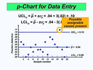
37. © 2008 Prentice Hall, Inc. S6 – 37
.11
.11 –
.10
.10 –
.09
.09 –
.08
.08 –
.07
.07 –
.06
.06 –
.05
.05 –
.04
.04 –
.03
.03 –
.02
.02 –
.01
.01 –
.00
.00 –
Sample number
Sample number
Fraction
defective
Fraction
defective
| | | | | | | | | |
2
2 4
4 6
6 8
8 10
10 12
12 14
14 16
16 18
18 20
20
p-Chart for Data Entry
p-Chart for Data Entry
UCL
UCLp
p = p + z
= p + z
p
p = .04 + 3(.02) = .10
= .04 + 3(.02) = .10
^
^
LCL
LCLp
p = p - z
= p - z
p
p = .04 - 3(.02) = 0
= .04 - 3(.02) = 0
^
^
UCL
UCLp
p = 0.10
= 0.10
LCL
LCLp
p = 0.00
= 0.00
p
p = 0.04
= 0.04

38. © 2008 Prentice Hall, Inc. S6 – 38
p-Chart for Data Entry
p-Chart for Data Entry
.11
.11 –
.10
.10 –
.09
.09 –
.08
.08 –
.07
.07 –
.06
.06 –
.05
.05 –
.04
.04 –
.03
.03 –
.02
.02 –
.01
.01 –
.00
.00 –
Sample number
Sample number
Fraction
defective
Fraction
defective
| | | | | | | | | |
2
2 4
4 6
6 8
8 10
10 12
12 14
14 16
16 18
18 20
20
UCL
UCLp
p = p + z
= p + z
p
p = .04 + 3(.02) = .10
= .04 + 3(.02) = .10
^
^
LCL
LCLp
p = p - z
= p - z
p
p = .04 - 3(.02) = 0
= .04 - 3(.02) = 0
^
^
UCL
UCLp
p = 0.10
= 0.10
LCL
LCLp
p = 0.00
= 0.00
p
p = 0.04
= 0.04
Possible
assignable
causes present

39. © 2008 Prentice Hall, Inc. S6 – 39
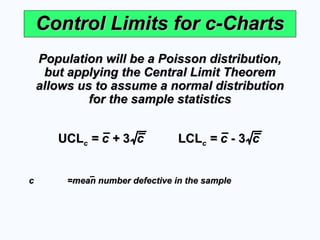
Control Limits for c-Charts
Control Limits for c-Charts
Population will be a Poisson distribution,
Population will be a Poisson distribution,
but applying the Central Limit Theorem
but applying the Central Limit Theorem
allows us to assume a normal distribution
allows us to assume a normal distribution
for the sample statistics
for the sample statistics
c
c =
=mean number defective in the sample
mean number defective in the sample
UCL
UCLc
c = c +
= c + 3
3 c
c LCL
LCLc
c = c
= c -
- 3
3 c
c

40. © 2008 Prentice Hall, Inc. S6 – 40
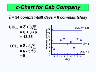
c-Chart for Cab Company
c-Chart for Cab Company
c
c = 54
= 54 complaints
complaints/9
/9 days
days = 6
= 6 complaints
complaints/
/day
day
|
1
|
2
|
3
|
4
|
5
|
6
|
7
|
8
|
9
Day
Day
Number
defective
Number
defective
14
14 –
12
12 –
10
10 –
8
8 –
6
6 –
4 –
2 –
0
0 –
UCL
UCLc
c = c +
= c + 3
3 c
c
= 6 + 3 6
= 6 + 3 6
= 13.35
= 13.35
LCL
LCLc
c = c -
= c - 3
3 c
c
= 6 - 3 6
= 6 - 3 6
= 0
= 0
UCL
UCLc
c = 13.35
= 13.35
LCL
LCLc
c = 0
= 0
c
c = 6
= 6

41. © 2008 Prentice Hall, Inc. S6 – 41
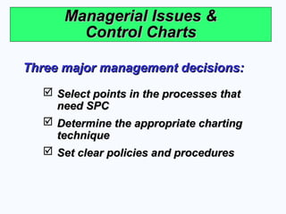
Managerial Issues &
Managerial Issues &
Control Charts
Control Charts
 Select points in the processes that
Select points in the processes that
need SPC
need SPC
 Determine the appropriate charting
Determine the appropriate charting
technique
technique
 Set clear policies and procedures
Set clear policies and procedures
Three major management decisions:
Three major management decisions:

42. © 2008 Prentice Hall, Inc. S6 – 42
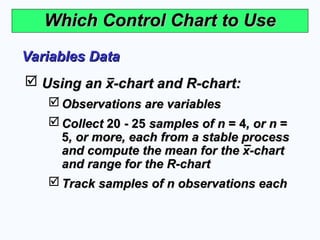
Which Control Chart to Use
Which Control Chart to Use
 Using an x-chart and R-chart:
Using an x-chart and R-chart:
 Observations are variables
Observations are variables
 Collect
Collect 20 - 25
20 - 25 samples of n
samples of n = 4
= 4, or n
, or n =
=
5
5, or more, each from a stable process
, or more, each from a stable process
and compute the mean for the x-chart
and compute the mean for the x-chart
and range for the R-chart
and range for the R-chart
 Track samples of n observations each
Track samples of n observations each
Variables Data
Variables Data

43. © 2008 Prentice Hall, Inc. S6 – 43
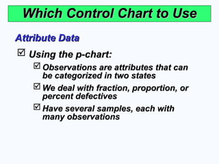
Which Control Chart to Use
Which Control Chart to Use
 Using the p-chart:
Using the p-chart:
 Observations are attributes that can
Observations are attributes that can
be categorized in two states
be categorized in two states
 We deal with fraction, proportion, or
We deal with fraction, proportion, or
percent defectives
percent defectives
 Have several samples, each with
Have several samples, each with
many observations
many observations
Attribute Data
Attribute Data

44. © 2008 Prentice Hall, Inc. S6 – 44
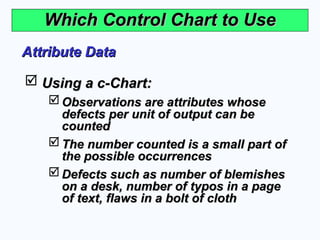
Which Control Chart to Use
Which Control Chart to Use
 Using a c-Chart:
Using a c-Chart:
 Observations are attributes whose
Observations are attributes whose
defects per unit of output can be
defects per unit of output can be
counted
counted
 The number counted is a small part of
The number counted is a small part of
the possible occurrences
the possible occurrences
 Defects such as number of blemishes
Defects such as number of blemishes
on a desk, number of typos in a page
on a desk, number of typos in a page
of text, flaws in a bolt of cloth
of text, flaws in a bolt of cloth
Attribute Data
Attribute Data

45. © 2008 Prentice Hall, Inc. S6 – 45
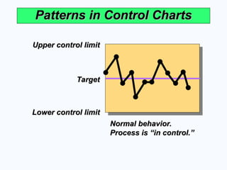
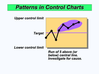
Patterns in Control Charts
Patterns in Control Charts
Normal behavior.
Normal behavior.
Process is “in control.”
Process is “in control.”
Upper control limit
Upper control limit
Target
Target
Lower control limit
Lower control limit

46. © 2008 Prentice Hall, Inc. S6 – 46
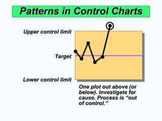
Patterns in Control Charts
Patterns in Control Charts
Upper control limit
Upper control limit
Target
Target
Lower control limit
Lower control limit
One plot out above (or
One plot out above (or
below). Investigate for
below). Investigate for
cause. Process is “out
cause. Process is “out
of control.”
of control.”

47. © 2008 Prentice Hall, Inc. S6 – 47
Upper control limit
Upper control limit
Target
Target
Lower control limit
Lower control limit
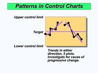
Patterns in Control Charts
Patterns in Control Charts
Trends in either
Trends in either
direction, 5 plots.
direction, 5 plots.
Investigate for cause of
Investigate for cause of
progressive change.
progressive change.

48. © 2008 Prentice Hall, Inc. S6 – 48
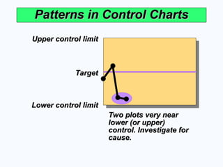
Patterns in Control Charts
Patterns in Control Charts
Upper control limit
Upper control limit
Target
Target
Lower control limit
Lower control limit
Two plots very near
Two plots very near
lower (or upper)
lower (or upper)
control. Investigate for
control. Investigate for
cause.
cause.

49. © 2008 Prentice Hall, Inc. S6 – 49
Patterns in Control Charts
Patterns in Control Charts
Upper control limit
Upper control limit
Target
Target
Lower control limit
Lower control limit
Run of 5 above (or
Run of 5 above (or
below) central line.
below) central line.
Investigate for cause.
Investigate for cause.

50. © 2008 Prentice Hall, Inc. S6 – 50
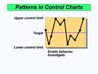
Patterns in Control Charts
Patterns in Control Charts
Upper control limit
Upper control limit
Target
Target
Lower control limit
Lower control limit
Erratic behavior.
Erratic behavior.
Investigate.
Investigate.

51. © 2008 Prentice Hall, Inc. S6 – 51
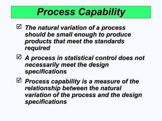
Process Capability
Process Capability
 The natural variation of a process
The natural variation of a process
should be small enough to produce
should be small enough to produce
products that meet the standards
products that meet the standards
required
required
 A process in statistical control does not
A process in statistical control does not
necessarily meet the design
necessarily meet the design
specifications
specifications
 Process capability is a measure of the
Process capability is a measure of the
relationship between the natural
relationship between the natural
variation of the process and the design
variation of the process and the design
specifications
specifications

52. © 2008 Prentice Hall, Inc. S6 – 52
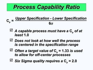
Process Capability Ratio
Process Capability Ratio
C
Cp
p =
=
Upper Specification - Lower Specification
Upper Specification - Lower Specification
6
6

 A capable process must have a
A capable process must have a C
Cp
p of at
of at
least
least 1.0
1.0
 Does not look at how well the process
Does not look at how well the process
is centered in the specification range
is centered in the specification range
 Often a target value of
Often a target value of C
Cp
p = 1.33
= 1.33 is used
is used
to allow for off-center processes
to allow for off-center processes
 Six Sigma quality requires a
Six Sigma quality requires a C
Cp
p = 2.0
= 2.0

53. © 2008 Prentice Hall, Inc. S6 – 53
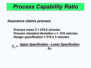
Process Capability Ratio
Process Capability Ratio
C
Cp
p =
=
Upper Specification - Lower Specification
Upper Specification - Lower Specification
6
6

Insurance claims process
Insurance claims process
Process mean x
Process mean x = 210.0
= 210.0 minutes
minutes
Process standard deviation
Process standard deviation 
 = .516
= .516 minutes
minutes
Design specification
Design specification = 210 ± 3
= 210 ± 3 minutes
minutes

54. © 2008 Prentice Hall, Inc. S6 – 54
Process Capability Ratio
Process Capability Ratio
C
Cp
p =
=
Upper Specification - Lower Specification
Upper Specification - Lower Specification
6
6

Insurance claims process
Insurance claims process
Process mean x
Process mean x = 210.0
= 210.0 minutes
minutes
Process standard deviation
Process standard deviation 
 = .516
= .516 minutes
minutes
Design specification
Design specification = 210 ± 3
= 210 ± 3 minutes
minutes
= = 1.938
= = 1.938
213 - 207
213 - 207
6(.516)
6(.516)

55. © 2008 Prentice Hall, Inc. S6 – 55
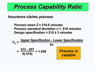
Process Capability Ratio
Process Capability Ratio
C
Cp
p =
=
Upper Specification - Lower Specification
Upper Specification - Lower Specification
6
6

Insurance claims process
Insurance claims process
Process mean x
Process mean x = 210.0
= 210.0 minutes
minutes
Process standard deviation
Process standard deviation 
 = .516
= .516 minutes
minutes
Design specification
Design specification = 210 ± 3
= 210 ± 3 minutes
minutes
= = 1.938
= = 1.938
213 - 207
213 - 207
6(.516)
6(.516)
Process is
capable

56. © 2008 Prentice Hall, Inc. S6 – 56
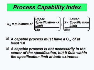
Process Capability Index
Process Capability Index
 A capable process must have a
A capable process must have a C
Cpk
pk of at
of at
least
least 1.0
1.0
 A capable process is not necessarily in the
A capable process is not necessarily in the
center of the specification, but it falls within
center of the specification, but it falls within
the specification limit at both extremes
the specification limit at both extremes
C
Cpk
pk = minimum of ,
= minimum of ,
Upper
Upper
Specification - x
Specification - x
Limit
Limit


Lower
Lower
x -
x - Specification
Specification
Limit
Limit



57. © 2008 Prentice Hall, Inc. S6 – 57
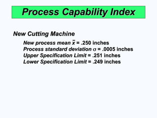
Process Capability Index
Process Capability Index
New Cutting Machine
New Cutting Machine
New process mean x
New process mean x = .250 inches
= .250 inches
Process standard deviation
Process standard deviation 
 = .0005 inches
= .0005 inches
Upper Specification Limit
Upper Specification Limit = .251 inches
= .251 inches
Lower Specification Limit
Lower Specification Limit = .249 inches
= .249 inches

58. © 2008 Prentice Hall, Inc. S6 – 58
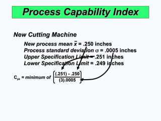
Process Capability Index
Process Capability Index
New Cutting Machine
New Cutting Machine
New process mean x
New process mean x = .250 inches
= .250 inches
Process standard deviation
Process standard deviation 
 = .0005 inches
= .0005 inches
Upper Specification Limit
Upper Specification Limit = .251 inches
= .251 inches
Lower Specification Limit
Lower Specification Limit = .249 inches
= .249 inches
C
Cpk
pk = minimum of ,
= minimum of ,
(.251) - .250
(.251) - .250
(3).0005
(3).0005

59. © 2008 Prentice Hall, Inc. S6 – 59
Process Capability Index
Process Capability Index
New Cutting Machine
New Cutting Machine
New process mean x
New process mean x = .250 inches
= .250 inches
Process standard deviation
Process standard deviation 
 = .0005 inches
= .0005 inches
Upper Specification Limit
Upper Specification Limit = .251 inches
= .251 inches
Lower Specification Limit
Lower Specification Limit = .249 inches
= .249 inches
C
Cpk
pk = = 0.67
= = 0.67
.001
.001
.0015
.0015
New machine is
NOT capable
C
Cpk
pk = minimum of ,
= minimum of ,
(.251) - .250
(.251) - .250
(3).0005
(3).0005
.250 - (.249)
.250 - (.249)
(3).0005
(3).0005
Both calculations result in
Both calculations result in

60. © 2008 Prentice Hall, Inc. S6 – 60
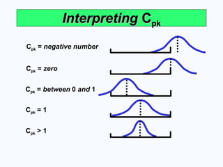
Interpreting
Interpreting C
Cpk
pk
Cpk = negative number
Cpk = zero
Cpk = between 0 and 1
Cpk = 1
Cpk > 1

61. © 2008 Prentice Hall, Inc. S6 – 61
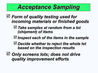
Acceptance Sampling
Acceptance Sampling
 Form of quality testing used for
Form of quality testing used for
incoming materials or finished goods
incoming materials or finished goods
 Take samples at random from a lot
Take samples at random from a lot
(shipment) of items
(shipment) of items
 Inspect each of the items in the sample
Inspect each of the items in the sample
 Decide whether to reject the whole lot
Decide whether to reject the whole lot
based on the inspection results
based on the inspection results
 Only screens lots; does not drive
Only screens lots; does not drive
quality improvement efforts
quality improvement efforts

62. © 2008 Prentice Hall, Inc. S6 – 62
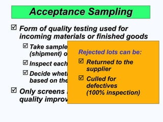
Acceptance Sampling
Acceptance Sampling
 Form of quality testing used for
Form of quality testing used for
incoming materials or finished goods
incoming materials or finished goods
 Take samples at random from a lot
Take samples at random from a lot
(shipment) of items
(shipment) of items
 Inspect each of the items in the sample
Inspect each of the items in the sample
 Decide whether to reject the whole lot
Decide whether to reject the whole lot
based on the inspection results
based on the inspection results
 Only screens lots; does not drive
Only screens lots; does not drive
quality improvement efforts
quality improvement efforts
Rejected lots can be:
 Returned to the
supplier
 Culled for
defectives
(100% inspection)

63. © 2008 Prentice Hall, Inc. S6 – 63
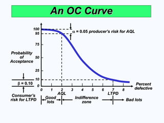
Operating Characteristic Curve
Operating Characteristic Curve
 Shows how well a sampling plan
Shows how well a sampling plan
discriminates between good and
discriminates between good and
bad lots (shipments)
bad lots (shipments)
 Shows the relationship between
Shows the relationship between
the probability of accepting a lot
the probability of accepting a lot
and its quality level
and its quality level

64. © 2008 Prentice Hall, Inc. S6 – 64
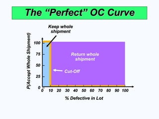
The “Perfect” OC Curve
The “Perfect” OC Curve
Return whole
shipment
% Defective in Lot
% Defective in Lot
P(Accept
Whole
Shipment)
P(Accept
Whole
Shipment)
100
100 –
75
75 –
50
50 –
25
25 –
0
0 –
| | | | | | | | | | |
0
0 10
10 20
20 30
30 40
40 50
50 60
60 70
70 80
80 90
90 100
100
Cut-Off
Keep whole
Keep whole
shipment
shipment

65. © 2008 Prentice Hall, Inc. S6 – 65
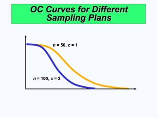
An OC Curve
An OC Curve
Probability
Probability
of
of
Acceptance
Acceptance
Percent
Percent
defective
defective
| | | | | | | | |
0
0 1
1 2
2 3
3 4
4 5
5 6
6 7
7 8
8
100
100 –
95
95 –
75
75 –
50
50 –
25
25 –
10
10 –
0
0 –

 = 0.05
= 0.05 producer’s risk for AQL
producer’s risk for AQL

 = 0.10
= 0.10
Consumer’s
Consumer’s
risk for LTPD
risk for LTPD
LTPD
LTPD
AQL
AQL
Bad lots
Bad lots
Indifference
Indifference
zone
zone
Good
Good
lots
lots

66. © 2008 Prentice Hall, Inc. S6 – 66
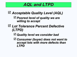
AQL and LTPD
AQL and LTPD
 Acceptable Quality Level (AQL)
Acceptable Quality Level (AQL)
 Poorest level of quality we are
Poorest level of quality we are
willing to accept
willing to accept
 Lot Tolerance Percent Defective
Lot Tolerance Percent Defective
(LTPD)
(LTPD)
 Quality level we consider bad
Quality level we consider bad
 Consumer (buyer) does not want to
Consumer (buyer) does not want to
accept lots with more defects than
accept lots with more defects than
LTPD
LTPD

67. © 2008 Prentice Hall, Inc. S6 – 67
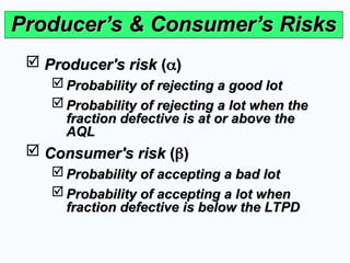
Producer’s & Consumer’s Risks
Producer’s & Consumer’s Risks
 Producer's risk
Producer's risk (
(
)
)
 Probability of rejecting a good lot
Probability of rejecting a good lot
 Probability of rejecting a lot when the
Probability of rejecting a lot when the
fraction defective is at or above the
fraction defective is at or above the
AQL
AQL
 Consumer's risk
Consumer's risk (
(
)
)
 Probability of accepting a bad lot
Probability of accepting a bad lot
 Probability of accepting a lot when
Probability of accepting a lot when
fraction defective is below the LTPD
fraction defective is below the LTPD

68. © 2008 Prentice Hall, Inc. S6 – 68
OC Curves for Different
OC Curves for Different
Sampling Plans
Sampling Plans
n
n = 50,
= 50, c
c = 1
= 1
n
n = 100,
= 100, c
c = 2
= 2

69. © 2008 Prentice Hall, Inc. S6 – 69
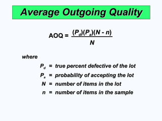
Average Outgoing Quality
Average Outgoing Quality
where
where
P
Pd
d = true percent defective of the lot
= true percent defective of the lot
P
Pa
a = probability of accepting the lot
= probability of accepting the lot
N
N = number of items in the lot
= number of items in the lot
n
n = number of items in the sample
= number of items in the sample
AOQ =
AOQ = (
(P
Pd
d)(
)(P
Pa
a)(
)(N - n
N - n)
)
N
N

70. © 2008 Prentice Hall, Inc. S6 – 70
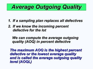
Average Outgoing Quality
Average Outgoing Quality
1.
1. If a sampling plan replaces all defectives
If a sampling plan replaces all defectives
2.
2. If we know the incoming percent
If we know the incoming percent
defective for the lot
defective for the lot
We can compute the average outgoing
We can compute the average outgoing
quality (AOQ) in percent defective
quality (AOQ) in percent defective
The maximum AOQ is the highest percent
The maximum AOQ is the highest percent
defective or the lowest average quality
defective or the lowest average quality
and is called the average outgoing quality
and is called the average outgoing quality
level (AOQL)
level (AOQL)

71. © 2008 Prentice Hall, Inc. S6 – 71
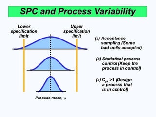
SPC and Process Variability
SPC and Process Variability
(a)
(a) Acceptance
Acceptance
sampling (Some
sampling (Some
bad units accepted)
bad units accepted)
(b)
(b) Statistical process
Statistical process
control (Keep the
control (Keep the
process in control)
process in control)
(c)
(c) C
Cpk
pk >1
>1 (Design
(Design
a process that
a process that
is in control)
is in control)
Lower
Lower
specification
specification
limit
limit
Upper
Upper
specification
specification
limit
limit
Process mean,
Process mean, 


72. © 2008 Prentice Hall, Inc. S6 – 72
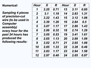
Numerical:
Numerical:
Sampling 4 pieces
Sampling 4 pieces
of precision-cut
of precision-cut
wire (to be used in
wire (to be used in
Computer
Computer
assembly)
assembly)
every hour for the
every hour for the
past 24 hours has
past 24 hours has
produced the
produced the
following results:
following results:
Hour
Hour X
X R
R Hour
Hour X
X R
R
1
1 3.25
3.25 0.71
0.71 13
13 3.11
3.11 0.85
0.85
2
2 3.1
3.1 1.18
1.18 14
14 2.83
2.83 1.31
1.31
3
3 3.22
3.22 1.43
1.43 15
15 3.12
3.12 1.06
1.06
4
4 3.39
3.39 1.26
1.26 16
16 2.84
2.84 0.5
0.5
5
5 3.07
3.07 1.17
1.17 17
17 2.86
2.86 1.43
1.43
6
6 2.86
2.86 0.32
0.32 18
18 2.74
2.74 1.29
1.29
7
7 3.05
3.05 0.53
0.53 19
19 3.41
3.41 1.61
1.61
8
8 2.65
2.65 1.13
1.13 20
20 2.89
2.89 1.09
1.09
9
9 3.02
3.02 0.71
0.71 21
21 2.65
2.65 1.08
1.08
10
10 2.85
2.85 1.33
1.33 22
22 3.28
3.28 0.46
0.46
11
11 2.83
2.83 1.17
1.17 23
23 2.94
2.94 1.58
1.58
12
12 2.97
2.97 0.40
0.40 24
24 2.65
2.65 0.97
0.97

73. © 2008 Prentice Hall, Inc. S6 – 73
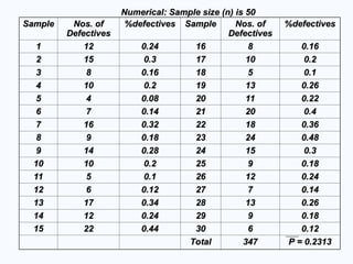
Sample
Sample Nos. of
Nos. of
Defectives
Defectives
%defectives
%defectives Sample
Sample Nos. of
Nos. of
Defectives
Defectives
%defectives
%defectives
1
1 12
12 0.24
0.24 16
16 8
8 0.16
0.16
2
2 15
15 0.3
0.3 17
17 10
10 0.2
0.2
3
3 8
8 0.16
0.16 18
18 5
5 0.1
0.1
4
4 10
10 0.2
0.2 19
19 13
13 0.26
0.26
5
5 4
4 0.08
0.08 20
20 11
11 0.22
0.22
6
6 7
7 0.14
0.14 21
21 20
20 0.4
0.4
7
7 16
16 0.32
0.32 22
22 18
18 0.36
0.36
8
8 9
9 0.18
0.18 23
23 24
24 0.48
0.48
9
9 14
14 0.28
0.28 24
24 15
15 0.3
0.3
10
10 10
10 0.2
0.2 25
25 9
9 0.18
0.18
11
11 5
5 0.1
0.1 26
26 12
12 0.24
0.24
12
12 6
6 0.12
0.12 27
27 7
7 0.14
0.14
13
13 17
17 0.34
0.34 28
28 13
13 0.26
0.26
14
14 12
12 0.24
0.24 29
29 9
9 0.18
0.18
15
15 22
22 0.44
0.44 30
30 6
6 0.12
0.12
Total
Total 347
347 P = 0.2313
P = 0.2313
Numerical: Sample size (n) is 50
Numerical: Sample size (n) is 50

74. © 2008 Prentice Hall, Inc. S6 – 74
If we know the probability of part produced
If we know the probability of part produced
being defective is p OR this is a standard then
being defective is p OR this is a standard then
we don’t need to calculate %defective.
we don’t need to calculate %defective.
If n=50, and p = 0.24
If n=50, and p = 0.24
then
then
calculate UCL and LCL for the control charts.
calculate UCL and LCL for the control charts.