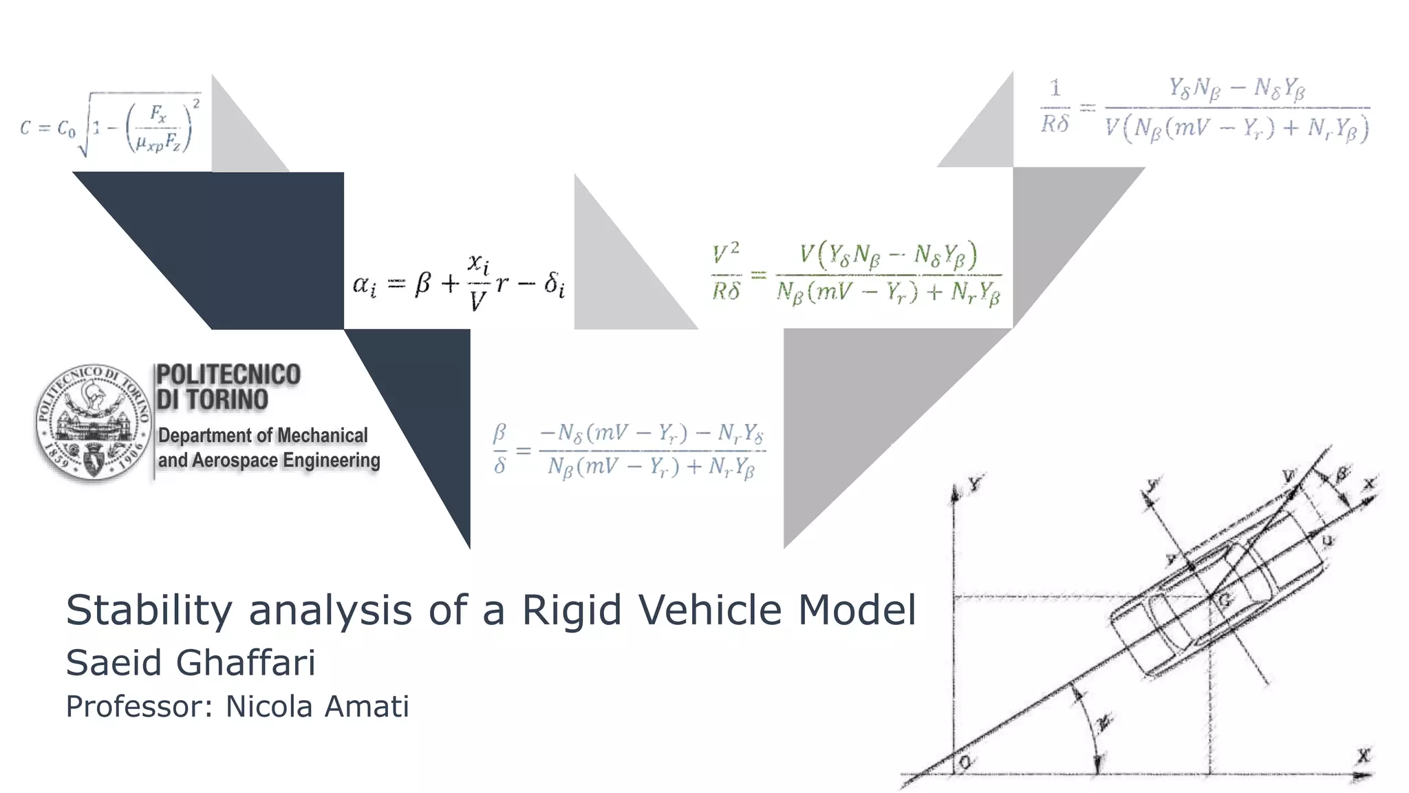
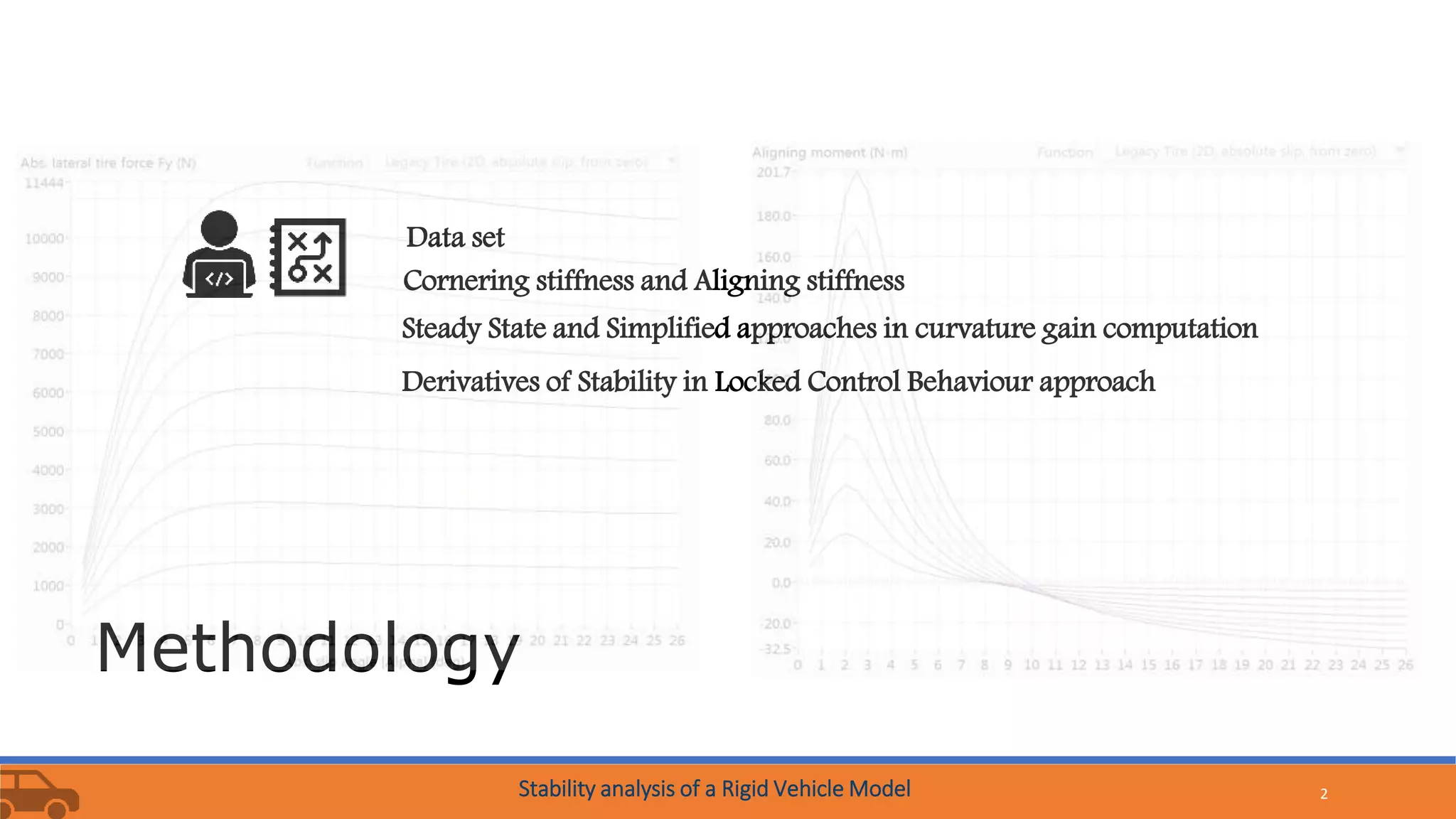
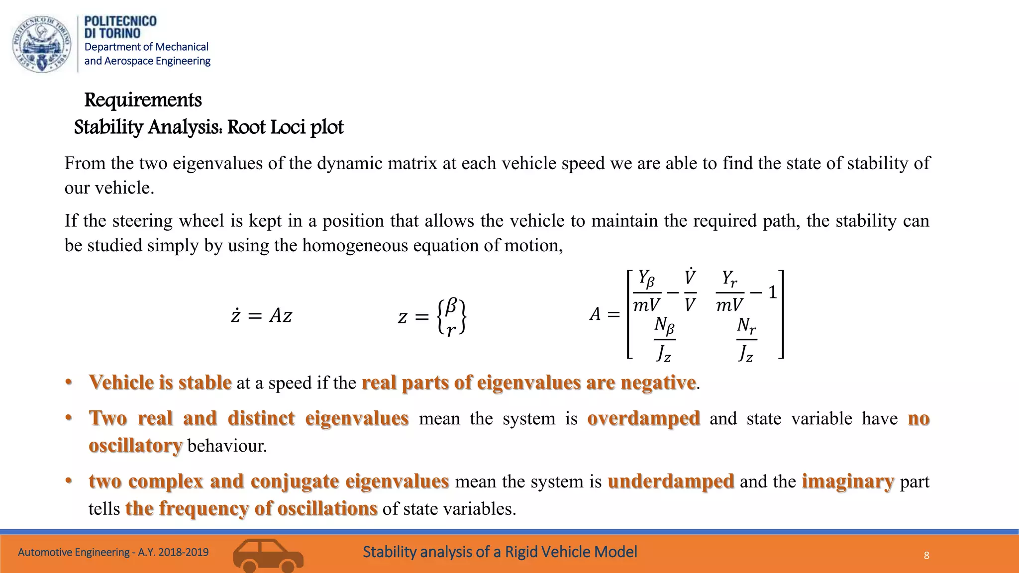
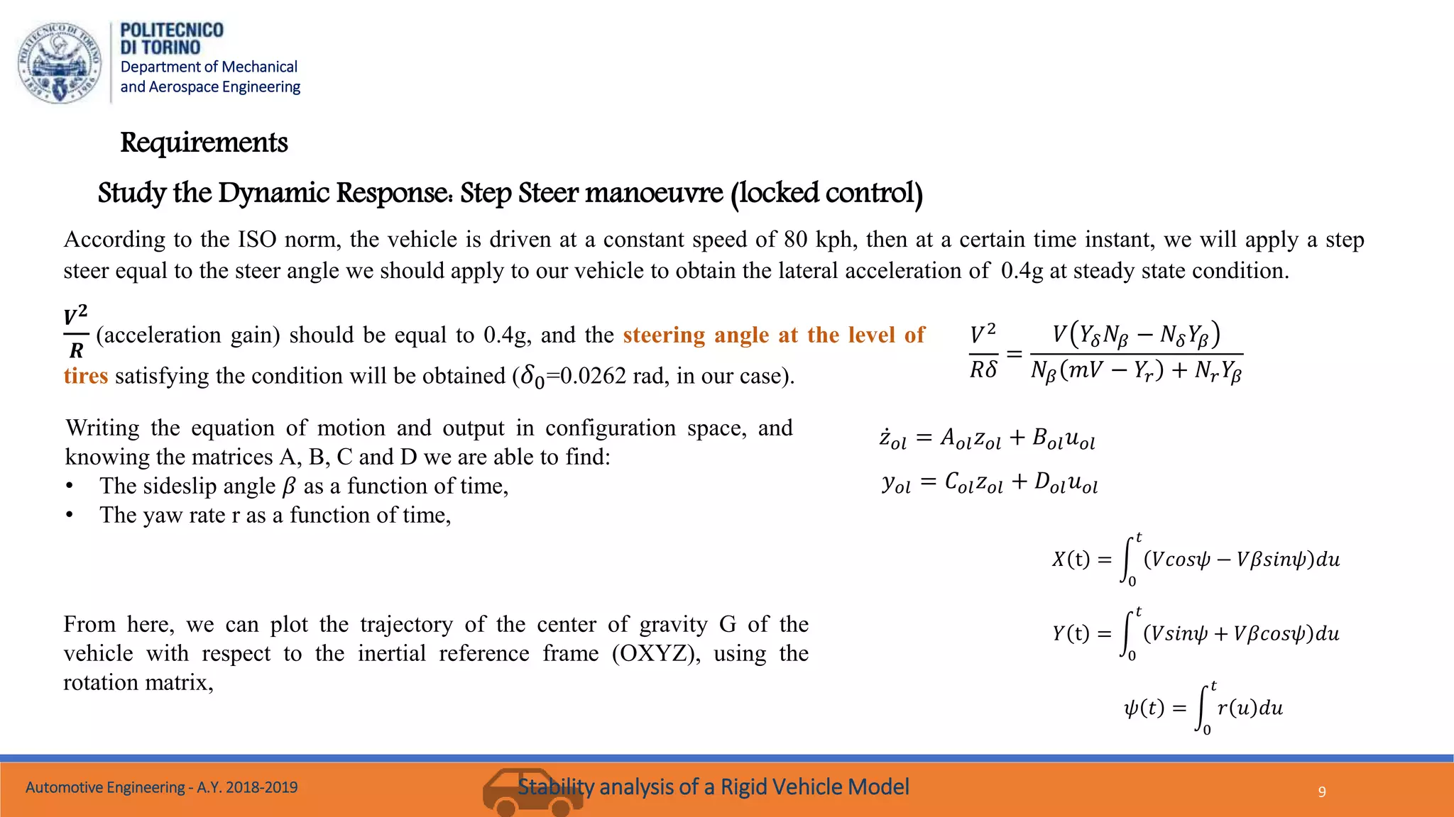
Stability analysis of a Rigid Vehicle Model
Department of Mechanical
and Aerospace Engineering
Saeid Ghaffari
Professor: Nicola Amati
2
Methodology
Data set
Cornering stiffness and Aligning stiffness
Steady State and Simplified approaches in curvature gain computation
Derivatives of Stability in Locked Control Behaviour approach
Stability analysis of a Rigid Vehicle Model
Automotive Engineering - A.Y. 2018-2019
Department of Mechanical
and Aerospace Engineering
3
Methodology
Characteristic Value (unit)
Acceleration of
gravity
9.81 (m/s2)
Sprung mass 1370 (kg)
Unsprung mass
Front axle
80 (kg)
Unsprung mass
rear axle
80 (kg)
Yaw moment of
inertia
2315.3 (kgm2)
Wheel base 2.780 (m)
Front axle to CG 1.110 (m)
Height of CG 0.520 (m)
Wheel track 1.550 (m)
Characteristic Value (unit)
Density of air 1.206 (kg/m3)
Front area 2.3 (m2)
Lateral aerodynamic force
coefficient
-0.5
Aerodynamic coefficient
about z
-0.05
Starting from a D-class sedan with the following characteristics, we will be able to find the requirements of the analysis.
Data set
Stability analysis of a Rigid Vehicle Model
Department of Mechanical
and Aerospace Engineering
4
Methodology
Regarding the aligning moment (𝑀𝑧) versus sideslip angle (𝛼) diagram, according to
the axle vertical load with interpolation in linear range, we can find the slope at the
origin.
• Cornering stiffness of front and rear axle 𝑪 𝟏 and 𝑪 𝟐
From the diagram of lateral force (−𝐹𝑦) with respect to the sideslip angle (𝛼), derived
with zero traction force, considering the vertical load we can find cornering stiffnesses
with interpolation in linear range.
• Aligning stiffness for front and rear axles 𝑴 𝒛𝟏 𝜶 and 𝑴 𝒛𝟐 𝜶
Abs. sideslip angle (deg)
Characteristic* Value (unit)
Cornering stiffness (front axle) 144446 (N/rad)
Cornering stiffness (rear axle) 102764 (N/rad)
Aligning stiffness (front axle) 8978 (Nm/rad)
Aligning stiffness (rear axle) 8318 (Nm/rad)
* when we have zero longitudinal force
Based on the interaction between the side force and
longitudinal force applied to a tire, applying the traction
force to a wheel, we will witness a modification into the
lateral stiffness according to its vertical load.
Elliptical Approach
𝑪 = 𝑪 𝟎 𝟏 −
𝑭 𝒙
𝝁 𝒙𝒑 𝑭 𝒛
𝟐
Automotive Engineering - A.Y. 2018-2019 Stability analysis of a Rigid Vehicle Model
Department of Mechanical
and Aerospace Engineering
5
Methodology
High- speed cornering (Dynamic steering) Steady State condition
Simplified approach Complete approach
Considering only tires’ cornering stiffness
Allows one to obtain a fair approximation
of the directional behaviour of the vehicle
Both aligning torques of tires (𝑀𝑧1 and
𝑀𝑧2) and the marginal effects of
aerodynamic forces and moments
𝟏
𝑹𝜹
=
𝟏
𝒍
𝒍
𝟏 + 𝑲 𝒖𝒔
𝑽 𝟐
𝒍𝒈
𝑽 𝟐
𝑹𝜹
=
𝑽 𝟐
𝒍
𝒍
𝟏 + 𝑲 𝒖𝒔
𝑽 𝟐
𝒍𝒈
𝜷
𝜹
=
𝒃
𝒍
(𝟏 −
𝒎𝒂𝑽 𝟐
𝟏 + 𝒃𝒍𝑪 𝟐
)
𝒍
𝟏 + 𝑲 𝒖𝒔
𝑽 𝟐
𝒍𝒈
𝟏
𝑹𝜹
=
𝒀 𝜹 𝑵 𝜷 − 𝑵 𝜹 𝒀 𝜷
𝑽 𝑵 𝜷 𝒎𝑽 − 𝒀 𝒓 + 𝑵 𝒓 𝒀 𝜷
𝑽 𝟐
𝑹𝜹
=
𝑽 𝒀 𝜹 𝑵 𝜷 − 𝑵 𝜹 𝒀 𝜷
𝑵 𝜷 𝒎𝑽 − 𝒀 𝒓 + 𝑵 𝒓 𝒀 𝜷
𝜷
𝜹
=
−𝑵 𝜹(𝒎𝑽 − 𝒀 𝒓) − 𝑵 𝒓 𝒀 𝜹
𝑵 𝜷(𝒎𝑽 − 𝒀 𝒓) + 𝑵 𝒓 𝒀 𝜷
Automotive Engineering - A.Y. 2018-2019 Stability analysis of a Rigid Vehicle Model
Department of Mechanical
and Aerospace Engineering
6
Methodology
High- speed cornering (Dynamic steering) Steady State condition
Considering the maximum amount of torque coming from the gearbox, we can evaluate the maximum amount of traction force on the
axle,
Case 1: Total traction force is applied to the front wheels, (𝐹𝑥1 = 620 𝑁)
Case 2: Total traction force is applied to the rear wheels, (𝐹𝑥2 = 620 𝑁)
Case 3: Half of the traction force is applied to the front wheels and half of it to the rear ones (𝐹𝑥1 = 310 𝑁) and (𝐹𝑥2 = 310 𝑁).
It is requested to assess the effects of two different states of loading on the whole problem:
• Traction Force
• Transversal Load Transfer
We will consider 25% load transfer from left wheels to the right wheels. New values for cornering stiffness and aligning stiffness for
each wheel will be found interpolating between the data coming from the CarSim.
Evaluating the derivatives of stability with new values of stiffness will lead to find the new transfer functions of lateral dynamic behaviour.
Automotive Engineering - A.Y. 2018-2019 Stability analysis of a Rigid Vehicle Model
Department of Mechanical
and Aerospace Engineering
7
Requirements
Steady-state Lateral Dynamic behaviour (over/under steering)
Simplified approach Complete approach
Considering only tires’ cornering stiffness
Allows one to obtain a fair approximation
of the directional behaviour of the vehicle
Both aligning torques of tires (𝑀𝑧1 and
𝑀𝑧2) and the marginal effects of
aerodynamic forces and moments
𝟏
𝑹𝜹
=
𝟏
𝒍
𝒍
𝟏 + 𝑲 𝒖𝒔
𝑽 𝟐
𝒍𝒈
𝟏
𝑹𝜹
=
𝒀 𝜹 𝑵 𝜷 − 𝑵 𝜹 𝒀 𝜷
𝑽 𝑵 𝜷 𝒎𝑽 − 𝒀 𝒓 + 𝑵 𝒓 𝒀 𝜷
Automotive Engineering - A.Y. 2018-2019 Stability analysis of a Rigid Vehicle Model
Department of Mechanical
and Aerospace Engineering
8
Requirements
From the two eigenvalues of the dynamic matrix at each vehicle speed we are able to find the state of stability of
our vehicle.
If the steering wheel is kept in a position that allows the vehicle to maintain the required path, the stability can
be studied simply by using the homogeneous equation of motion,
𝑧 = 𝐴𝑧 𝑧 =
𝛽
𝑟
𝐴 =
𝑌𝛽
𝑚𝑉
−
𝑉
𝑉
𝑌𝑟
𝑚𝑉
− 1
𝑁𝛽
𝐽𝑧
𝑁𝑟
𝐽𝑧
• Vehicle is stable at a speed if the real parts of eigenvalues are negative.
• Two real and distinct eigenvalues mean the system is overdamped and state variable have no
oscillatory behaviour.
• two complex and conjugate eigenvalues mean the system is underdamped and the imaginary part
tells the frequency of oscillations of state variables.
Stability Analysis: Root Loci plot
Automotive Engineering - A.Y. 2018-2019 Stability analysis of a Rigid Vehicle Model
Department of Mechanical
and Aerospace Engineering
9
Requirements
Study the Dynamic Response: Step Steer manoeuvre (locked control)
According to the ISO norm, the vehicle is driven at a constant speed of 80 kph, then at a certain time instant, we will apply a step
steer equal to the steer angle we should apply to our vehicle to obtain the lateral acceleration of 0.4g at steady state condition.
𝑉2
𝑅𝛿
=
𝑉 𝑌𝛿 𝑁𝛽 − 𝑁𝛿 𝑌𝛽
𝑁𝛽 𝑚𝑉 − 𝑌𝑟 + 𝑁𝑟 𝑌𝛽
𝑽 𝟐
𝑹
(acceleration gain) should be equal to 0.4g, and the steering angle at the level of
tires satisfying the condition will be obtained ( 𝛿0=0.0262 rad, in our case).
From here, we can plot the trajectory of the center of gravity G of the
vehicle with respect to the inertial reference frame (OXYZ), using the
rotation matrix,
𝑋 t =
0
𝑡
𝑉𝑐𝑜𝑠𝜓 − 𝑉𝛽𝑠𝑖𝑛𝜓 𝑑𝑢
𝑌 t =
0
𝑡
𝑉𝑠𝑖𝑛𝜓 + 𝑉𝛽𝑐𝑜𝑠𝜓 𝑑𝑢
𝜓 𝑡 =
0
𝑡
𝑟 𝑢 𝑑𝑢
Writing the equation of motion and output in configuration space, and
knowing the matrices A, B, C and D we are able to find:
• The sideslip angle 𝛽 as a function of time,
• The yaw rate r as a function of time,
𝑧 𝑜𝑙 = 𝐴 𝑜𝑙 𝑧 𝑜𝑙 + 𝐵 𝑜𝑙 𝑢 𝑜𝑙
𝑦 𝑜𝑙 = 𝐶 𝑜𝑙 𝑧 𝑜𝑙 + 𝐷 𝑜𝑙 𝑢 𝑜𝑙
Automotive Engineering - A.Y. 2018-2019 Stability analysis of a Rigid Vehicle Model
Results and discussion
Traction Force (𝑭 𝒙𝟏=620 N) is applied to the Front Axle
Traction Force (𝑭 𝒙𝟐=620 N) is applied to the Rear Axle
Traction Force is applied equally to the Front and Rear Axle (𝑭 𝒙𝟏=310 N, 𝑭 𝒙𝟐=310 N)
Transversal Load Transfer effects on lateral dynamics behaviors
Root loci as a function of the vehicle speed (traction force)
Root loci as a function of the vehicle speed (transversal load transfer)
Steady-state dynamic response to Step Steer maneuver
Steady-state Lateral behavior
Sideslip angle time history
Yaw rate time history
Trajectory

Stability analysis of a Rigid Vehicle Model

  • 1.
    Stability analysis ofa Rigid Vehicle Model Department of Mechanical and Aerospace Engineering Saeid Ghaffari Professor: Nicola Amati
  • 2.
    2 Methodology Data set Cornering stiffnessand Aligning stiffness Steady State and Simplified approaches in curvature gain computation Derivatives of Stability in Locked Control Behaviour approach Stability analysis of a Rigid Vehicle Model
  • 3.
    Automotive Engineering -A.Y. 2018-2019 Department of Mechanical and Aerospace Engineering 3 Methodology Characteristic Value (unit) Acceleration of gravity 9.81 (m/s2) Sprung mass 1370 (kg) Unsprung mass Front axle 80 (kg) Unsprung mass rear axle 80 (kg) Yaw moment of inertia 2315.3 (kgm2) Wheel base 2.780 (m) Front axle to CG 1.110 (m) Height of CG 0.520 (m) Wheel track 1.550 (m) Characteristic Value (unit) Density of air 1.206 (kg/m3) Front area 2.3 (m2) Lateral aerodynamic force coefficient -0.5 Aerodynamic coefficient about z -0.05 Starting from a D-class sedan with the following characteristics, we will be able to find the requirements of the analysis. Data set Stability analysis of a Rigid Vehicle Model
  • 4.
    Department of Mechanical andAerospace Engineering 4 Methodology Regarding the aligning moment (𝑀𝑧) versus sideslip angle (𝛼) diagram, according to the axle vertical load with interpolation in linear range, we can find the slope at the origin. • Cornering stiffness of front and rear axle 𝑪 𝟏 and 𝑪 𝟐 From the diagram of lateral force (−𝐹𝑦) with respect to the sideslip angle (𝛼), derived with zero traction force, considering the vertical load we can find cornering stiffnesses with interpolation in linear range. • Aligning stiffness for front and rear axles 𝑴 𝒛𝟏 𝜶 and 𝑴 𝒛𝟐 𝜶 Abs. sideslip angle (deg) Characteristic* Value (unit) Cornering stiffness (front axle) 144446 (N/rad) Cornering stiffness (rear axle) 102764 (N/rad) Aligning stiffness (front axle) 8978 (Nm/rad) Aligning stiffness (rear axle) 8318 (Nm/rad) * when we have zero longitudinal force Based on the interaction between the side force and longitudinal force applied to a tire, applying the traction force to a wheel, we will witness a modification into the lateral stiffness according to its vertical load. Elliptical Approach 𝑪 = 𝑪 𝟎 𝟏 − 𝑭 𝒙 𝝁 𝒙𝒑 𝑭 𝒛 𝟐 Automotive Engineering - A.Y. 2018-2019 Stability analysis of a Rigid Vehicle Model
  • 5.
    Department of Mechanical andAerospace Engineering 5 Methodology High- speed cornering (Dynamic steering) Steady State condition Simplified approach Complete approach Considering only tires’ cornering stiffness Allows one to obtain a fair approximation of the directional behaviour of the vehicle Both aligning torques of tires (𝑀𝑧1 and 𝑀𝑧2) and the marginal effects of aerodynamic forces and moments 𝟏 𝑹𝜹 = 𝟏 𝒍 𝒍 𝟏 + 𝑲 𝒖𝒔 𝑽 𝟐 𝒍𝒈 𝑽 𝟐 𝑹𝜹 = 𝑽 𝟐 𝒍 𝒍 𝟏 + 𝑲 𝒖𝒔 𝑽 𝟐 𝒍𝒈 𝜷 𝜹 = 𝒃 𝒍 (𝟏 − 𝒎𝒂𝑽 𝟐 𝟏 + 𝒃𝒍𝑪 𝟐 ) 𝒍 𝟏 + 𝑲 𝒖𝒔 𝑽 𝟐 𝒍𝒈 𝟏 𝑹𝜹 = 𝒀 𝜹 𝑵 𝜷 − 𝑵 𝜹 𝒀 𝜷 𝑽 𝑵 𝜷 𝒎𝑽 − 𝒀 𝒓 + 𝑵 𝒓 𝒀 𝜷 𝑽 𝟐 𝑹𝜹 = 𝑽 𝒀 𝜹 𝑵 𝜷 − 𝑵 𝜹 𝒀 𝜷 𝑵 𝜷 𝒎𝑽 − 𝒀 𝒓 + 𝑵 𝒓 𝒀 𝜷 𝜷 𝜹 = −𝑵 𝜹(𝒎𝑽 − 𝒀 𝒓) − 𝑵 𝒓 𝒀 𝜹 𝑵 𝜷(𝒎𝑽 − 𝒀 𝒓) + 𝑵 𝒓 𝒀 𝜷 Automotive Engineering - A.Y. 2018-2019 Stability analysis of a Rigid Vehicle Model
  • 6.
    Department of Mechanical andAerospace Engineering 6 Methodology High- speed cornering (Dynamic steering) Steady State condition Considering the maximum amount of torque coming from the gearbox, we can evaluate the maximum amount of traction force on the axle, Case 1: Total traction force is applied to the front wheels, (𝐹𝑥1 = 620 𝑁) Case 2: Total traction force is applied to the rear wheels, (𝐹𝑥2 = 620 𝑁) Case 3: Half of the traction force is applied to the front wheels and half of it to the rear ones (𝐹𝑥1 = 310 𝑁) and (𝐹𝑥2 = 310 𝑁). It is requested to assess the effects of two different states of loading on the whole problem: • Traction Force • Transversal Load Transfer We will consider 25% load transfer from left wheels to the right wheels. New values for cornering stiffness and aligning stiffness for each wheel will be found interpolating between the data coming from the CarSim. Evaluating the derivatives of stability with new values of stiffness will lead to find the new transfer functions of lateral dynamic behaviour. Automotive Engineering - A.Y. 2018-2019 Stability analysis of a Rigid Vehicle Model
  • 7.
    Department of Mechanical andAerospace Engineering 7 Requirements Steady-state Lateral Dynamic behaviour (over/under steering) Simplified approach Complete approach Considering only tires’ cornering stiffness Allows one to obtain a fair approximation of the directional behaviour of the vehicle Both aligning torques of tires (𝑀𝑧1 and 𝑀𝑧2) and the marginal effects of aerodynamic forces and moments 𝟏 𝑹𝜹 = 𝟏 𝒍 𝒍 𝟏 + 𝑲 𝒖𝒔 𝑽 𝟐 𝒍𝒈 𝟏 𝑹𝜹 = 𝒀 𝜹 𝑵 𝜷 − 𝑵 𝜹 𝒀 𝜷 𝑽 𝑵 𝜷 𝒎𝑽 − 𝒀 𝒓 + 𝑵 𝒓 𝒀 𝜷 Automotive Engineering - A.Y. 2018-2019 Stability analysis of a Rigid Vehicle Model
  • 8.
    Department of Mechanical andAerospace Engineering 8 Requirements From the two eigenvalues of the dynamic matrix at each vehicle speed we are able to find the state of stability of our vehicle. If the steering wheel is kept in a position that allows the vehicle to maintain the required path, the stability can be studied simply by using the homogeneous equation of motion, 𝑧 = 𝐴𝑧 𝑧 = 𝛽 𝑟 𝐴 = 𝑌𝛽 𝑚𝑉 − 𝑉 𝑉 𝑌𝑟 𝑚𝑉 − 1 𝑁𝛽 𝐽𝑧 𝑁𝑟 𝐽𝑧 • Vehicle is stable at a speed if the real parts of eigenvalues are negative. • Two real and distinct eigenvalues mean the system is overdamped and state variable have no oscillatory behaviour. • two complex and conjugate eigenvalues mean the system is underdamped and the imaginary part tells the frequency of oscillations of state variables. Stability Analysis: Root Loci plot Automotive Engineering - A.Y. 2018-2019 Stability analysis of a Rigid Vehicle Model
  • 9.
    Department of Mechanical andAerospace Engineering 9 Requirements Study the Dynamic Response: Step Steer manoeuvre (locked control) According to the ISO norm, the vehicle is driven at a constant speed of 80 kph, then at a certain time instant, we will apply a step steer equal to the steer angle we should apply to our vehicle to obtain the lateral acceleration of 0.4g at steady state condition. 𝑉2 𝑅𝛿 = 𝑉 𝑌𝛿 𝑁𝛽 − 𝑁𝛿 𝑌𝛽 𝑁𝛽 𝑚𝑉 − 𝑌𝑟 + 𝑁𝑟 𝑌𝛽 𝑽 𝟐 𝑹 (acceleration gain) should be equal to 0.4g, and the steering angle at the level of tires satisfying the condition will be obtained ( 𝛿0=0.0262 rad, in our case). From here, we can plot the trajectory of the center of gravity G of the vehicle with respect to the inertial reference frame (OXYZ), using the rotation matrix, 𝑋 t = 0 𝑡 𝑉𝑐𝑜𝑠𝜓 − 𝑉𝛽𝑠𝑖𝑛𝜓 𝑑𝑢 𝑌 t = 0 𝑡 𝑉𝑠𝑖𝑛𝜓 + 𝑉𝛽𝑐𝑜𝑠𝜓 𝑑𝑢 𝜓 𝑡 = 0 𝑡 𝑟 𝑢 𝑑𝑢 Writing the equation of motion and output in configuration space, and knowing the matrices A, B, C and D we are able to find: • The sideslip angle 𝛽 as a function of time, • The yaw rate r as a function of time, 𝑧 𝑜𝑙 = 𝐴 𝑜𝑙 𝑧 𝑜𝑙 + 𝐵 𝑜𝑙 𝑢 𝑜𝑙 𝑦 𝑜𝑙 = 𝐶 𝑜𝑙 𝑧 𝑜𝑙 + 𝐷 𝑜𝑙 𝑢 𝑜𝑙 Automotive Engineering - A.Y. 2018-2019 Stability analysis of a Rigid Vehicle Model
  • 10.
    Results and discussion TractionForce (𝑭 𝒙𝟏=620 N) is applied to the Front Axle Traction Force (𝑭 𝒙𝟐=620 N) is applied to the Rear Axle Traction Force is applied equally to the Front and Rear Axle (𝑭 𝒙𝟏=310 N, 𝑭 𝒙𝟐=310 N) Transversal Load Transfer effects on lateral dynamics behaviors Root loci as a function of the vehicle speed (traction force) Root loci as a function of the vehicle speed (transversal load transfer) Steady-state dynamic response to Step Steer maneuver Steady-state Lateral behavior Sideslip angle time history Yaw rate time history Trajectory

Editor's Notes

  • #3 The roll camber of the wheel has something to do with the Camber stiffness of tire And the roll steer of the wheel has something to do with the cornering stiffness of the tire (in N_phi equation)