1.6. 实现我们的⽹络来分类数字
函数 σ。(这称为将函数σ 向量化。)很容易验证⽅程 (22) 的结果和我们之前的计算⼀个 S 型神
经元输出的⽅程 (4) 相同。
练习
• 以分量形式写出⽅程 (22),并验证它和计算 S 型神经元输出的规则 (4) 结果相同。
有了这些,很容易写出从⼀个 Network 实例计算输出的代码。我们从定义 S 型函数开始:
def sigmoid(z):
return 1.0/(1.0+np.exp(-z))
注意,当输⼊ z 是⼀个向量或者 Numpy 数组时,Numpy ⾃动地按元素应⽤ sigmoid 函数,即
以向量形式。
我们然后对 Network 类添加⼀个 feedforward ⽅法,对于⽹络给定⼀个输⼊ a,返回对应的输
出6。这个⽅法所做的是对每⼀层应⽤⽅程 (22):
def feedforward(self, a):
"""Return the output of the network if "a" is input."""
for b, w in zip(self.biases, self.weights):
a = sigmoid(np.dot(w, a)+b)
return a
当然,我们想要 Network 对象做的主要事情是学习。为此我们给它们⼀个实现随即梯度下降
算法的 SGD ⽅法。代码如下。其中⼀些地⽅看似有⼀点神秘,我会在代码后⾯逐个分析。
def SGD(self, training_data, epochs, mini_batch_size, eta,
test_data=None):
"""Train the neural network using mini-batch stochastic
gradient descent. The "training_data" is a list of tuples
"(x, y)" representing the training inputs and the desired
outputs. The other non-optional parameters are
self-explanatory. If "test_data" is provided then the
network will be evaluated against the test data after each
epoch, and partial progress printed out. This is useful for
tracking progress, but slows things down substantially."""
if test_data: n_test = len(test_data)
n = len(training_data)
for j in xrange(epochs):
random.shuffle(training_data)
mini_batches = [
training_data[k:k+mini_batch_size]
for k in xrange(0, n, mini_batch_size)]
for mini_batch in mini_batches:
self.update_mini_batch(mini_batch, eta)
if test_data:
print "Epoch {0}: {1} / {2}".format(
j, self.evaluate(test_data), n_test)
else:
print "Epoch {0} complete".format(j)
training_data 是⼀个 (x, y) 元组的列表,表⽰训练输⼊和其对应的期望输出。变量 epochs 和
mini_batch_size 正如你预料的 —— 迭代期数量,和采样时的⼩批量数据的⼤⼩。eta 是学习速率,
η。如果给出了可选参数 test_data,那么程序会在每个训练器后评估⽹络,并打印出部分进展。
这对于追踪进度很有⽤,但相当拖慢执⾏速度。
6
这⾥假设输⼊ a 是⼀个 (n,1) 的 Numpy ndarray 类型,⽽不是⼀个 (n,) 的向量。这⾥,n 是⽹络的输⼊数量。
如果你试着⽤⼀个 (n,) 向量作为输⼊,会得到奇怪的结果。虽然使⽤ (n,) 向量看上去好像是更⾃然的选择,但是
使⽤⼀个 (n,1) 的 ndarray 使得修改代码来⽴即前馈多个输⼊变得特别容易,并且有的时候很⽅便。
22
33.
1.6. 实现我们的⽹络来分类数字
代码如下⼯作。在每个迭代期,它⾸先随机地将训练数据打乱,然后将它分成多个适当⼤
⼩的⼩批量数据。这是⼀个简单的从训练数据的随机采样⽅法。然后对于每⼀个 mini_batch
我们应⽤⼀次梯度下降。这是通过代码self.update_mini_batch(mini_batch, eta) 完成的,它仅
仅使⽤ mini_batch 中的训练数据,根据单次梯度下降的迭代更新⽹络的权重和偏置。这是
update_mini_batch ⽅法的代码:
def update_mini_batch(self, mini_batch, eta):
"""Update the network's weights and biases by applying
gradient descent using backpropagation to a single mini batch.
The "mini_batch" is a list of tuples "(x, y)", and "eta"
is the learning rate."""
nabla_b = [np.zeros(b.shape) for b in self.biases]
nabla_w = [np.zeros(w.shape) for w in self.weights]
for x, y in mini_batch:
delta_nabla_b, delta_nabla_w = self.backprop(x, y)
nabla_b = [nb+dnb for nb, dnb in zip(nabla_b, delta_nabla_b)]
nabla_w = [nw+dnw for nw, dnw in zip(nabla_w, delta_nabla_w)]
self.weights = [w-(eta/len(mini_batch))*nw
for w, nw in zip(self.weights, nabla_w)]
self.biases = [b-(eta/len(mini_batch))*nb
for b, nb in zip(self.biases, nabla_b)]
⼤部分⼯作由这⾏代码完成:
delta_nabla_b, delta_nabla_w = self.backprop(x, y)
这⾏调⽤了⼀个称为反向传播的算法,⼀种快速计算代价函数的梯度的⽅法。因此
update_mini_batch 的⼯作仅仅是对 mini_batch 中的每⼀个训练样本计算梯度,然后适当地更
新 self.weights 和 self.biases。
我现在不会列出 self.backprop 的代码。我们将在下章中学习反向传播是怎样⼯作的,包括
self.backprop 的代码。现在,就假设它按照我们要求的⼯作,返回与训练样本 x 相关代价的适
当梯度。
让我们看⼀下完整的程序,包括我之前忽略的⽂档注释。除了 self.backprop,程序已经有了
⾜够的⽂档注释 —— 所有的繁重⼯作由 self.SGD 和 self.update_mini_batch 完成,对此我们已经
有讨论过。self.backprop ⽅法利⽤⼀些额外的函数来帮助计算梯度,即 sigmoid_prime,它计算 σ
函数的导数,以及 self.cost_derivative,这⾥我不会对它过多描述。你能够通过查看代码或⽂
档注释来获得这些的要点(或者细节)。我们将在下章详细地看它们。注意,虽然程序显得很⻓,
但是很多代码是⽤来使代码更容易理解的⽂档注释。实际上,程序只包含 74 ⾏⾮空、⾮注释的
代码。所有的代码可以在 GitHub 上这⾥找到。
"""
network.py
~~~~~~~~~~
A module to implement the stochastic gradient descent learning
algorithm for a feedforward neural network. Gradients are calculated
using backpropagation. Note that I have focused on making the code
simple, easily readable, and easily modifiable. It is not optimized,
and omits many desirable features.
"""
#### Libraries
# Standard library
import random
# Third-party libraries
23
34.
1.6. 实现我们的⽹络来分类数字
import numpyas np
class Network(object):
def __init__(self, sizes):
"""The list ``sizes`` contains the number of neurons in the
respective layers of the network. For example, if the list
was [2, 3, 1] then it would be a three-layer network, with the
first layer containing 2 neurons, the second layer 3 neurons,
and the third layer 1 neuron. The biases and weights for the
network are initialized randomly, using a Gaussian
distribution with mean 0, and variance 1. Note that the first
layer is assumed to be an input layer, and by convention we
won't set any biases for those neurons, since biases are only
ever used in computing the outputs from later layers."""
self.num_layers = len(sizes)
self.sizes = sizes
self.biases = [np.random.randn(y, 1) for y in sizes[1:]]
self.weights = [np.random.randn(y, x)
for x, y in zip(sizes[:-1], sizes[1:])]
def feedforward(self, a):
"""Return the output of the network if ``a`` is input."""
for b, w in zip(self.biases, self.weights):
a = sigmoid(np.dot(w, a)+b)
return a
def SGD(self, training_data, epochs, mini_batch_size, eta,
test_data=None):
"""Train the neural network using mini-batch stochastic
gradient descent. The ``training_data`` is a list of tuples
``(x, y)`` representing the training inputs and the desired
outputs. The other non-optional parameters are
self-explanatory. If ``test_data`` is provided then the
network will be evaluated against the test data after each
epoch, and partial progress printed out. This is useful for
tracking progress, but slows things down substantially."""
if test_data: n_test = len(test_data)
n = len(training_data)
for j in xrange(epochs):
random.shuffle(training_data)
mini_batches = [
training_data[k:k+mini_batch_size]
for k in xrange(0, n, mini_batch_size)]
for mini_batch in mini_batches:
self.update_mini_batch(mini_batch, eta)
if test_data:
print "Epoch {0}: {1} / {2}".format(
j, self.evaluate(test_data), n_test)
else:
print "Epoch {0} complete".format(j)
def update_mini_batch(self, mini_batch, eta):
"""Update the network's weights and biases by applying
gradient descent using backpropagation to a single mini batch.
The ``mini_batch`` is a list of tuples ``(x, y)``, and ``eta``
is the learning rate."""
nabla_b = [np.zeros(b.shape) for b in self.biases]
nabla_w = [np.zeros(w.shape) for w in self.weights]
for x, y in mini_batch:
delta_nabla_b, delta_nabla_w = self.backprop(x, y)
24
35.
1.6. 实现我们的⽹络来分类数字
nabla_b =[nb+dnb for nb, dnb in zip(nabla_b, delta_nabla_b)]
nabla_w = [nw+dnw for nw, dnw in zip(nabla_w, delta_nabla_w)]
self.weights = [w-(eta/len(mini_batch))*nw
for w, nw in zip(self.weights, nabla_w)]
self.biases = [b-(eta/len(mini_batch))*nb
for b, nb in zip(self.biases, nabla_b)]
def backprop(self, x, y):
"""Return a tuple ``(nabla_b, nabla_w)`` representing the
gradient for the cost function C_x. ``nabla_b`` and
``nabla_w`` are layer-by-layer lists of numpy arrays, similar
to ``self.biases`` and ``self.weights``."""
nabla_b = [np.zeros(b.shape) for b in self.biases]
nabla_w = [np.zeros(w.shape) for w in self.weights]
# feedforward
activation = x
activations = [x] # list to store all the activations, layer by layer
zs = [] # list to store all the z vectors, layer by layer
for b, w in zip(self.biases, self.weights):
z = np.dot(w, activation)+b
zs.append(z)
activation = sigmoid(z)
activations.append(activation)
# backward pass
delta = self.cost_derivative(activations[-1], y) *
sigmoid_prime(zs[-1])
nabla_b[-1] = delta
nabla_w[-1] = np.dot(delta, activations[-2].transpose())
# Note that the variable l in the loop below is used a little
# differently to the notation in Chapter 2 of the book. Here,
# l = 1 means the last layer of neurons, l = 2 is the
# second-last layer, and so on. It's a renumbering of the
# scheme in the book, used here to take advantage of the fact
# that Python can use negative indices in lists.
for l in xrange(2, self.num_layers):
z = zs[-l]
sp = sigmoid_prime(z)
delta = np.dot(self.weights[-l+1].transpose(), delta) * sp
nabla_b[-l] = delta
nabla_w[-l] = np.dot(delta, activations[-l-1].transpose())
return (nabla_b, nabla_w)
def evaluate(self, test_data):
"""Return the number of test inputs for which the neural
network outputs the correct result. Note that the neural
network's output is assumed to be the index of whichever
neuron in the final layer has the highest activation."""
test_results = [(np.argmax(self.feedforward(x)), y)
for (x, y) in test_data]
return sum(int(x == y) for (x, y) in test_results)
def cost_derivative(self, output_activations, y):
"""Return the vector of partial derivatives partial C_x /
partial a for the output activations."""
return (output_activations-y)
#### Miscellaneous functions
def sigmoid(z):
"""The sigmoid function."""
return 1.0/(1.0+np.exp(-z))
25
1.6. 实现我们的⽹络来分类数字
从这得到的教训是调试⼀个神经⽹络不是琐碎的,就像常规编程那样,它是⼀⻔艺术。你需
要学习调试的艺术来获得神经⽹络更好的结果。更普通的是,我们需要启发式⽅法来选择好的
超参数和好的结构。我们将在整本书中讨论这些,包括上⾯我是怎么样选择超参数的。
练习
• 试着创建⼀个仅有两层的⽹络—— ⼀个输⼊层和⼀个输出层,分别有 784 和 10 个神经元,
没有隐藏层。⽤随机梯度下降算法训练⽹络。你能达到多少识别率?
之前的内容中,我跳过了如何加载 MNIST 数据的细节。这很简单。这⾥列出了完整的代
码。⽤于存储 MNIST 数据的数据结构在⽂档注释中有详细描述 —— 都是简单的类型,元组和
Numpy ndarry 对象的列表(如果你不熟悉 ndarray,那就把它们看成向量):
"""
mnist_loader
~~~~~~~~~~~~
A library to load the MNIST image data. For details of the data
structures that are returned, see the doc strings for ``load_data``
and ``load_data_wrapper``. In practice, ``load_data_wrapper`` is the
function usually called by our neural network code.
"""
#### Libraries
# Standard library
import cPickle
import gzip
# Third-party libraries
import numpy as np
def load_data():
"""Return the MNIST data as a tuple containing the training data,
the validation data, and the test data.
The ``training_data`` is returned as a tuple with two entries.
The first entry contains the actual training images. This is a
numpy ndarray with 50,000 entries. Each entry is, in turn, a
numpy ndarray with 784 values, representing the 28 * 28 = 784
pixels in a single MNIST image.
The second entry in the ``training_data`` tuple is a numpy ndarray
containing 50,000 entries. Those entries are just the digit
values (0...9) for the corresponding images contained in the first
entry of the tuple.
The ``validation_data`` and ``test_data`` are similar, except
each contains only 10,000 images.
This is a nice data format, but for use in neural networks it's
helpful to modify the format of the ``training_data`` a little.
That's done in the wrapper function ``load_data_wrapper()``, see
below.
"""
f = gzip.open('../data/mnist.pkl.gz', 'rb')
training_data, validation_data, test_data = cPickle.load(f)
f.close()
return (training_data, validation_data, test_data)
28
39.
1.6. 实现我们的⽹络来分类数字
def load_data_wrapper():
"""Returna tuple containing ``(training_data, validation_data,
test_data)``. Based on ``load_data``, but the format is more
convenient for use in our implementation of neural networks.
In particular, ``training_data`` is a list containing 50,000
2-tuples ``(x, y)``. ``x`` is a 784-dimensional numpy.ndarray
containing the input image. ``y`` is a 10-dimensional
numpy.ndarray representing the unit vector corresponding to the
correct digit for ``x``.
``validation_data`` and ``test_data`` are lists containing 10,000
2-tuples ``(x, y)``. In each case, ``x`` is a 784-dimensional
numpy.ndarry containing the input image, and ``y`` is the
corresponding classification, i.e., the digit values (integers)
corresponding to ``x``.
Obviously, this means we're using slightly different formats for
the training data and the validation / test data. These formats
turn out to be the most convenient for use in our neural network
code."""
tr_d, va_d, te_d = load_data()
training_inputs = [np.reshape(x, (784, 1)) for x in tr_d[0]]
training_results = [vectorized_result(y) for y in tr_d[1]]
training_data = zip(training_inputs, training_results)
validation_inputs = [np.reshape(x, (784, 1)) for x in va_d[0]]
validation_data = zip(validation_inputs, va_d[1])
test_inputs = [np.reshape(x, (784, 1)) for x in te_d[0]]
test_data = zip(test_inputs, te_d[1])
return (training_data, validation_data, test_data)
def vectorized_result(j):
"""Return a 10-dimensional unit vector with a 1.0 in the jth
position and zeroes elsewhere. This is used to convert a digit
(0...9) into a corresponding desired output from the neural
network."""
e = np.zeros((10, 1))
e[j] = 1.0
return e
上⾯我说过我们的程序取得了⾮常好的结果。那意味着什么?和什么相⽐算好?如果有⼀些
简单的(⾮神经⽹络的)基线测试作为对⽐就有助于理解它怎样算运⾏良好。最简单的基线,当
然是随机地猜些数字。那将有 10% 的次数是正确的。我们将⽐这做得更好!
⼀个较差的基线会怎样?让我们尝试⼀种极其简单的想法:我们会看⼀幅图像有多暗。例如,
⼀幅 2 的图像通常要⽐⼀幅 1 的图像稍暗些,仅仅因为更多像素被涂⿊了,就像下⾯的⽰例显
⽰的:
这提⽰我们可以⽤训练数据来计算数字图像的平均暗度,0, 1, 2, . . . , 9。当有⼀幅新的图像
呈现,我们先计算图像的暗度,然后猜测它接近哪个数字的平均暗度。这是⼀个简单的程序,
⽽且容易编写代码,所以我不会在这⾥把它们都写出来 —— 如果你有兴趣,代码在 GitHub 仓
库⾥。但是它和随机地猜测相⽐有了很⼤的改进,能取得 10, 000 测试图像中 2, 225 的精确度,
即 22.25%。
29
1.7. 迈向深度学习
望在构建⼈⼯智能的努⼒过程中,也同时能够帮助我们理解智能背后的机制,以及⼈类⼤脑的
运转⽅式。但结果可能是我们既不能够理解⼤脑的机制,也不能够理解⼈⼯智能的机制。
为解决这些问题,让我们重新思考⼀下我在本章开始时所给的⼈⼯神经元的解释,作为⼀种
衡量证据的⽅法。假设我们要确定⼀幅图像是否显⽰有⼈脸8:
我们可以⽤解决⼿写识别问题的相同⽅式来攻克这个问题 ——⽹络的输⼊是图像中的像素,
⽹络的输出是⼀个单个的神经元⽤于表明“是的,这是⼀张脸”或“不,这不是⼀张脸”。
假设我们就采取了这个⽅法,但接下来我们先不去使⽤⼀个学习算法。⽽是去尝试亲⼿设计
⼀个⽹络,并为它选择合适的权重和偏置。我们要怎样做呢?暂时先忘掉神经⽹络,我们受到
启发的⼀个想法是将这个问题分解成⼦问题:图像的左上⻆有⼀个眼睛吗?右上⻆有⼀个眼睛
吗?中间有⼀个⿐⼦吗?下⾯中央有⼀个嘴吗?上⾯有头发吗?诸如此类。
如果⼀些问题的回答是“是”,或者甚⾄仅仅是“可能是”,那么我们可以作出结论这个图像
可能是⼀张脸。相反地,如果⼤多数这些问题的答案是“不是”,那么这张图像可能不是⼀张脸。
当然,这仅仅是⼀个粗略的想法,⽽且它存在许多缺陷。也许有个⼈是秃头,没有头发。也
许我们仅仅能看到脸的部分,或者这张脸是有⻆度的,因此⼀些⾯部特征是模糊的。不过这个
想法表明了如果我们能够使⽤神经⽹络来解决这些⼦问题,那么我们也许可以通过将这些解决
⼦问题的⽹络结合起来,构成⼀个⼈脸检测的神经⽹络。下图是⼀个可能的结构,其中的⽅框
表⽰⼦⽹络。注意,这不是⼀个⼈脸检测问题的现实的解决⽅法,⽽是为了帮助我们构建起⽹
络如何运转的直观感受。下图是这个⽹络的结构:
8
照⽚来源:1. Ester Inbar. 2. 未知. 3. NASA, ESA, G. Illingworth, D. Magee, and P. Oesch (University of California,
Santa Cruz), R. Bouwens (Leiden University), and the HUDF09 Team. 点击序号查看更多细节。
31
2.6. 反向传播算法
简化上⼀个⽅程为:
δL
j =
∂C
∂aL
j
∂aL
j
∂zL
j
(38)
回想下aL
j = σ(zL
j ),右边的第⼆项可以写为 σ′(zL
j ),⽅程变成:
δL
j =
∂C
∂aL
j
σ′
(zL
j ) (39)
这正是分量形式的 (BP1)。
下⼀步,我们将证明 (BP2),它给出了以下⼀层误差 δl+1 的形式表⽰误差 δl。为此,我们想
要以 δl+1
k = ∂C/∂zl+1
k 的形式重写 δl
j = ∂C/∂zl
j。我们可以⽤链式法则:
δl
j =
∂C
∂zl
j
(40)
=
∑
k
∂C
∂zl+1
k
∂zl+1
k
∂zl
j
(41)
=
∑
k
∂zl+1
k
∂zl
j
δl+1
k (42)
这⾥最后⼀⾏我们交换了右边的两项,并⽤ δl+1
k 的定义代⼊。为了对最后⼀⾏的第⼀项求值,
注意:
zl+1
k =
∑
j
wl+1
kj al
j + bl+1
k =
∑
j
wl+1
kj σ(zl
j) + bl+1
k (43)
做微分,我们得到
∂zl+1
k
∂zl
j
= wl+1
kj σ′
(zl
j) (44)
把它代⼊ (42) 我们得到
δl
j =
∑
k
wl+1
kj δl+1
k σ′
(zl
j) (45)
这正是以分量形式写的 (BP2)。
我们想证明的最后两个⽅程是 (BP3) 和 (BP4)。它们同样遵循链式法则,和前⾯两个⽅程的
证明相似。我把它们留给你做为练习。
练习
• 证明⽅程 (BP3) 和 (BP4)。
这样我们就完成了反向传播四个基本公式的证明。证明本⾝看起来复杂。但是实际上就是细
⼼地应⽤链式法则。我们可以将反向传播看成是⼀种系统性地应⽤多元微积分中的链式法则来
计算代价函数的梯度的⽅式。这些就是反向传播理论上的内容 —— 剩下的是实现细节。
2.6 反向传播算法
反向传播⽅程给出了⼀种计算代价函数梯度的⽅法。让我们显式地⽤算法描述出来:
42
53.
2.7. 代码
1. 输⼊x: 为输⼊层设置对应的激活值 a1 。
2. 前向传播: 对每个 l = 2, 3, ..., L 计算相应的 zl = wlal−1 + bl 和 al = σ(zl)
3. 输出层误差 δL: 计算向量 δL = ∇aC ⊙ σ′(zL)
4. 反向误差传播: 对每个 l = L − 1, L − 2, ..., 2,计算 δl = ((wl+1)T δl+1) ⊙ σ′(zl)
5. 输出: 代价函数的梯度由 ∂C
∂wl
jk
= al−1
k δl
j 和 ∂C
∂bl
j
= δl
j 得出
检视这个算法,你可以看到为何它被称作反向传播。我们从最后⼀层开始向后计算误差向量
δl。这看起来有点奇怪,为何要从后⾯开始。但是如果你认真思考反向传播的证明,这种反向移
动其实是代价函数是⽹络输出的函数的结果。为了理解代价随前⾯层的权重和偏置变化的规律,
我们需要重复作⽤链式法则,反向地获得需要的表达式。
练习
• 使⽤单个修正的神经元的反向传播 假设我们改变⼀个前馈⽹络中的单个神经元,使得那
个神经元的输出是 f(
∑
j wjxj + b),其中 f 是和 S 型函数不同的某⼀函数。我们如何调整
反向传播算法?
• 线性神经元上的反向传播 假设我们将⾮线性神经元的 σ 函数替换为 σ(z) = z。重写反向
传播算法。
正如我们上⾯所讲的,反向传播算法对⼀个训练样本计算代价函数的梯度,C = Cx。在实践
中,通常将反向传播算法和诸如随机梯度下降这样的学习算法进⾏组合使⽤,我们会对许多训
练样本计算对应的梯度。特别地,给定⼀个⼤⼩为 m 的⼩批量数据,下⾯的算法在这个⼩批量
数据的基础上应⽤⼀步梯度下降学习算法:
1. 输⼊训练样本的集合
2. 对每个训练样本 x: 设置对应的输⼊激活 ax,1,并执⾏下⾯的步骤:
• 前向传播: 对每个 l = 2, 3, ..., L 计算 zx,l = wlax,l−1 + bl 和 ax,l = σ(zx,l)。
• 输出误差 δx,L: 计算向量 δx,L = ∇aCx ⊙ σ′(zx,L)。
• 反向传播误差: 对每个 l = L − 1, L − 2, ..., 2 计算 δx,l = ((wl+1)T δx,l+1) ⊙ σ′(zx,l)。
3. 梯度下降: 对每个 l = L − 1, L − 2, ..., 2 根据 wl → wl − η
m
∑
x δx,l(ax,l−1)T 和 bl →
bl − η
m
∑
x δx,l 更新权重和偏置。
当然,在实践中实现随机梯度下降,我们还需要⼀个产⽣训练样本的⼩批量数据的循环,还
有就是多重迭代期的循环。这⾥我们先省略了。
2.7 代码
理解了抽象的反向传播的理论知识,我们现在就可以学习上⼀章中使⽤的实现反向传播的
代码了。回想上⼀章的代码,需要研究的是在 Network 类中的 update_mini_batch 和 backprop ⽅法。
这些⽅法的代码其实是我们上⾯的算法描述的直接翻版。特别地,update_mini_batch ⽅法通过计
算当前 mini_batch 中的训练样本对 Network 的权重和偏置进⾏了更新:
43
54.
2.7. 代码
class Network(object):
...
defupdate_mini_batch(self, mini_batch, eta):
"""Update the network's weights and biases by applying
gradient descent using backpropagation to a single mini batch.
The "mini_batch" is a list of tuples "(x, y)", and "eta"
is the learning rate."""
nabla_b = [np.zeros(b.shape) for b in self.biases]
nabla_w = [np.zeros(w.shape) for w in self.weights]
for x, y in mini_batch:
delta_nabla_b, delta_nabla_w = self.backprop(x, y)
nabla_b = [nb+dnb for nb, dnb in zip(nabla_b, delta_nabla_b)]
nabla_w = [nw+dnw for nw, dnw in zip(nabla_w, delta_nabla_w)]
self.weights = [w-(eta/len(mini_batch))*nw
for w, nw in zip(self.weights, nabla_w)]
self.biases = [b-(eta/len(mini_batch))*nb
for b, nb in zip(self.biases, nabla_b)]
主要⼯作其实是在 delta_nabla_b,delta_nabla_w = self.backprop(x, y) 这⾥完成的,调⽤了
backprop ⽅法计算出了偏导数,∂Cx/∂bl
j 和 ∂Cx/∂wl
jk。backprop ⽅法跟上⼀节的算法基本⼀致。
这⾥只有个⼩⼩的差异 —— 我们使⽤⼀个略微不同的⽅式来索引神经⽹络的层。这个改变其实
是为了 Python 的特性 —— 负值索引的使⽤能够让我们从列表的最后往前遍历,如 l[-3] 其实是
列表中的倒数第三个元素。下⾯ backprop 的代码,和⼀些帮助函数⼀起,被⽤于计算 σ、导数 σ′
及代价函数的导数。所以理解了这些,我们就完全可以掌握所有的代码了。如果某些东西让你
困惑,你可能需要参考代码的原始描述(以及完整清单)。
class Network(object):
...
def backprop(self, x, y):
"""Return a tuple "(nabla_b, nabla_w)" representing the
gradient for the cost function C_x. "nabla_b" and
"nabla_w" are layer-by-layer lists of numpy arrays, similar
to "self.biases" and "self.weights"."""
nabla_b = [np.zeros(b.shape) for b in self.biases]
nabla_w = [np.zeros(w.shape) for w in self.weights]
# feedforward
activation = x
activations = [x] # list to store all the activations, layer by layer
zs = [] # list to store all the z vectors, layer by layer
for b, w in zip(self.biases, self.weights):
z = np.dot(w, activation)+b
zs.append(z)
activation = sigmoid(z)
activations.append(activation)
# backward pass
delta = self.cost_derivative(activations[-1], y) *
sigmoid_prime(zs[-1])
nabla_b[-1] = delta
nabla_w[-1] = np.dot(delta, activations[-2].transpose())
# Note that the variable l in the loop below is used a little
# differently to the notation in Chapter 2 of the book. Here,
# l = 1 means the last layer of neurons, l = 2 is the
# second-last layer, and so on. It's a renumbering of the
# scheme in the book, used here to take advantage of the fact
# that Python can use negative indices in lists.
for l in xrange(2, self.num_layers):
z = zs[-l]
sp = sigmoid_prime(z)
delta = np.dot(self.weights[-l+1].transpose(), delta) * sp
44
3.2. 过度拟合和规范化
如你所⻅,测试集和训练集上的准确率相⽐我们使⽤ 1,000 个训练数据时相差更⼩。特别地,
在训练数据上的最佳的分类准确率 97.86% 只⽐测试集上的 95.33% 准确率⾼了 1.53%。⽽之前
的例⼦中,这个差距是 17.73%!过度拟合仍然发⽣了,但是已经减轻了不少。我们的⽹络从训
练数据上更好地泛化到了测试数据上。⼀般来说,最好的降低过度拟合的⽅式之⼀就是增加训
练样本的量。有了⾜够的训练数据,就算是⼀个规模⾮常⼤的⽹络也不⼤容易过度拟合。不幸
的是,训练数据其实是很难或者很昂贵的资源,所以这不是⼀种太切实际的选择。
3.2.1 规范化
增加训练样本的数量是⼀种减轻过度拟合的⽅法。还有其他的⼀下⽅法能够减轻过度拟合的
程度吗?⼀种可⾏的⽅式就是降低⽹络的规模。然⽽,⼤的⽹络拥有⼀种⽐⼩⽹络更强的潜⼒,
所以这⾥存在⼀种应⽤冗余性的选项。
幸运的是,还有其他的技术能够缓解过度拟合,即使我们只有⼀个固定的⽹络和固定的训练
集合。这种技术就是规范化。本节,我会给出⼀种最为常⽤的规范化⼿段 —— 有时候被称为权
重衰减(weight decay)或者 L2 规范化。L2 规范化的想法是增加⼀个额外的项到代价函数上,
这个项叫做规范化项。下⾯是规范化的交叉熵:
C = −
1
n
∑
xj
[
yj ln aL
j + (1 − yj) ln(1 − aL
j )
]
+
λ
2n
∑
w
w2
(85)
其中第⼀个项就是常规的交叉熵的表达式。第⼆个现在加⼊的就是所有权重的平⽅的和。然
后使⽤⼀个因⼦ λ/2n 进⾏量化调整,其中 λ > 0 可以称为规范化参数,⽽ n 就是训练集合的⼤
⼩。我们会在后⾯讨论 λ 的选择策略。需要注意的是,规范化项⾥⾯并不包含偏置。这点我们
后⾯也会在讲述。
当然,对其他的代价函数也可以进⾏规范化,例如⼆次代价函数。类似的规范化的形式如下:
C =
1
2n
∑
x
∥y − aL
∥2
+
λ
2n
∑
w
w2
(86)
两者都可以写成这样:
C = C0 +
λ
2n
∑
w
w2
(87)
71
82.
3.2. 过度拟合和规范化
其中 C0是原始的代价函数。
直觉地看,规范化的效果是让⽹络倾向于学习⼩⼀点的权重,其他的东西都⼀样的。⼤的权
重只有能够给出代价函数第⼀项⾜够的提升时才被允许。换⾔之,规范化可以当做⼀种寻找⼩
的权重和最⼩化原始的代价函数之间的折中。这两部分之前相对的重要性就由 λ 的值来控制了:
λ 越⼩,就偏向于最⼩化原始代价函数,反之,倾向于⼩的权重。
现在,对于这样的折中为何能够减轻过度拟合还不是很清楚!但是,实际表现表明了这点。
我们会在下⼀节来回答这个问题。但现在,我们来看看⼀个规范化的确减轻过度拟合的例⼦。
为了构造这个例⼦,我们⾸先需要弄清楚如何将随机梯度下降算法应⽤在⼀个规范化的神经
⽹络上。特别地,我们需要知道如何计算对⽹络中所有权重和偏置的偏导数 ∂C/∂w 和 ∂C/∂b。
对⽅程 (87) 进⾏求偏导数得:
∂C
∂w
=
∂C0
∂w
+
λ
n
w (88)
∂C
∂b
=
∂C0
∂b
(89)
∂C0/∂w 和 ∂C0/∂b 可以通过反向传播进⾏计算,正如上⼀章中描述的那样。所以我们看到
其实计算规范化的代价函数的梯度是很简单的:仅仅需要反向传播,然后加上 λ
nw 得到所有权
重的偏导数。⽽偏置的偏导数就不要变化,所以偏置的梯度下降学习规则不会发⽣变化:
b → b − η
∂C0
∂b
(90)
权重的学习规则就变成:
w → w − η
∂C0
∂w
−
ηλ
n
w (91)
=
(
1 −
ηλ
n
)
w − η
∂C0
∂w
(92)
这正和通常的梯度下降学习规则相同,除了通过⼀个因⼦ 1 − ηλ
n 重新调整了权重 w。这种调
整有时被称为权重衰减,因为它使得权重变⼩。粗看,这样会导致权重会不断下降到 0。但是实
际不是这样的,因为如果在原始代价函数中造成下降的话其他的项可能会让权重增加。
好的,这就是梯度下降⼯作的原理。那么随机梯度下降呢?正如在没有规范化的随机梯度下
降中,我们可以通过平均 m 个训练样本的⼩批量数据来估计 ∂C0/∂w。因此,为了随机梯度下
降的规范化学习规则就变成(参考⽅程 (20))
w →
(
1 −
ηλ
n
)
w −
η
m
∑
x
∂Cx
∂w
(93)
其中后⾯⼀项是在训练样本的⼩批量数据 x 上进⾏的,⽽ Cx 是对每个训练样本的(⽆规范化的)
代价。这其实和之前通常的随机梯度下降的规则是⼀样的,除了有⼀个权重下降的因⼦ 1 − ηλ
n 。
最后,为了完整,我给出偏置的规范化的学习规则。这当然是和我们之前的⾮规范化的情形⼀
致了(参考公式 (21)),
b → b −
η
m
∑
x
∂Cx
∂b
(94)
这⾥求和也是在训练样本的⼩批量数据 x 上进⾏的。
72
3.4. 再看⼿写识别问题:代码
0 510 15 20 25 30
Epoch
86
88
90
92
94
96
98
100 Classification accuracy
Old approach to weight initialization
New approach to weight initialization
在这个情况下,两个曲线并没有重合。然⽽,我做的实验发现了其实就在⼀些额外的迭代期
后(这⾥没有展⽰)准确率其实也是⼏乎相同的。所以,基于这些实验,看起来提升的权重初始
化仅仅会加快训练,不会改变⽹络的最终性能。然⽽,在第四章,我们会看到⼀些例⼦⾥⾯使
⽤ 1/
√
nin 权重初始化的⻓期运⾏的结果要显著更优。因此,不仅仅能够带来训练速度的加快,
有时候在最终性能上也有很⼤的提升。
1/
√
nin 的权重初始化⽅法帮助我们提升了神经⽹络学习的⽅式。其他的权重初始化技术同
样也被提出,很多都是基于这个基本的思想。我不会在这⾥回顾其他的⽅法,因为 1/
√
nin 已经
可以⼯作得很好了。如果你感兴趣的话,我推荐你看看在 2012 年的 Yoshua Bengio 的论⽂22的
14 和 15 ⻚,以及相关的参考⽂献。
问题
• 将规范化和改进的权重初始化⽅法结合使⽤ L2 规范化有时候会⾃动给我们⼀些类似于新
的初始化⽅法的东西。假设我们使⽤旧的初始化权重的⽅法。考虑⼀个启发式的观点:(1)
假设 λ 不太⼩,训练的第⼀迭代期将会⼏乎被权重衰减统治;(2)如果 ηλ ≪ n,权重会
按照因⼦ exp(−ηλ/m) 每 迭代期衰减;(3)假设 λ 不太⼤,权重衰减会在权重降到 1/
√
n
的时候保持住,其中 n 是⽹络中权重的个数。论证这些条件都已经在本节给出图⽰的例⼦
中满⾜。
3.4 再看⼿写识别问题:代码
让我们实现本章讨论过的这些想法。我们将写出⼀个新的程序,network2.py,这是⼀个对第
⼀章中开发的 network.py 的改进版本。如果你没有仔细看过 network.py,那你可能会需要重读前
⾯关于这段代码的讨论。仅仅 74 ⾏代码,也很易懂。
和 network.py ⼀样,主要部分就是 Network 类了,我们⽤这个来表⽰神经⽹络。使⽤⼀个 sizes
的列表来对每个对应层进⾏初始化,默认使⽤交叉熵作为代价 cost 参数:
class Network(object):
def __init__(self, sizes, cost=CrossEntropyCost):
22
Practical Recommendations for Gradient-Based Training of Deep Architectures,作者为 Yoshua Bengio(2012)。
88
99.
3.4. 再看⼿写识别问题:代码
self.num_layers =len(sizes)
self.sizes = sizes
self.default_weight_initializer()
self.cost=cost
最开始⼏⾏⾥的 __init__ ⽅法的和 network.py 中⼀样,可以轻易弄懂。但是下⾯两⾏是新的,
我们需要知道他们到底做了什么。
我们先看看 default_weight_initializer ⽅法,使⽤了我们新式改进后的初始化权重⽅法。如
我们已经看到的,使⽤了均值为 0 ⽽标准差为 1/
√
n,n 为对应的输⼊连接个数。我们使⽤均值
为 0 ⽽标准差为 1 的⾼斯分布来初始化偏置。下⾯是代码:
def default_weight_initializer(self):
self.biases = [np.random.randn(y, 1) for y in self.sizes[1:]]
self.weights = [np.random.randn(y, x)/np.sqrt(x)
for x, y in zip(self.sizes[:-1], self.sizes[1:])]
为了理解这段代码,需要知道 np 就是进⾏线性代数运算的 Numpy 库。我们在程序的开头会
import Numpy。同样我们没有对第⼀层的神经元的偏置进⾏初始化。因为第⼀层其实是输⼊层,
所以不需要引⼊任何的偏置。我们在 network.py 中做了完全⼀样的事情。
作为 default_weight_initializer 的补充,我们同样包含了⼀个 large_weight_initializer ⽅法。
这个⽅法使⽤了第⼀章中的观点初始化了权重和偏置。代码也就仅仅是和 default_weight_initializer
差了⼀点点了:
def large_weight_initializer(self):
self.biases = [np.random.randn(y, 1) for y in self.sizes[1:]]
self.weights = [np.random.randn(y, x)
for x, y in zip(self.sizes[:-1], self.sizes[1:])]
我将 larger_weight_initializer ⽅法包含进来的原因也就是使得跟第⼀章的结果更容易⽐较。
我并没有考虑太多的推荐使⽤这个⽅法的实际情景。
初始化⽅法 __init__ 中的第⼆个新的东西就是我们初始化了 cost 属性。为了理解这个⼯作的
原理,让我们看⼀下⽤来表⽰交叉熵代价的类23:
class CrossEntropyCost(object):
@staticmethod
def fn(a, y):
return np.sum(np.nan_to_num(-y*np.log(a)-(1-y)*np.log(1-a)))
@staticmethod
def delta(z, a, y):
return (a-y)
让我们分解⼀下。第⼀个看到的是:即使使⽤的是交叉熵,数学上看,就是⼀个函数,这⾥我
们⽤ Python 的类⽽不是 Python 函数实现了它。为什么这样做呢?答案就是代价函数在我们的
⽹络中扮演了两种不同的⻆⾊。明显的⻆⾊就是代价是输出激活值 a 和⽬标输出 y 差距优劣的
度量。这个⻆⾊通过 CrossEntropyCost.fn ⽅法来扮演。(注意,np.nan_to_num 调⽤确保了 Numpy
正确处理接近 0 的对数值)但是代价函数其实还有另⼀个⻆⾊。回想第⼆章中运⾏反向传播算
法时,我们需要计算⽹络输出误差,δL。这种形式的输出误差依赖于代价函数的选择:不同的
23
如果你不熟悉 Python 的静态⽅法,你可以忽略 @staticmethod 装饰符,仅仅把 fn 和 delta 看作普通⽅法。如
果你想知道细节,所有的 @staticmethod 所做的是告诉 Python 解释器其随后的⽅法完全不依赖于对象。这就是为
什么 self 没有作为参数传⼊ fn 和 delta。
89
100.
3.4. 再看⼿写识别问题:代码
代价函数,输出误差的形式就不同。对于交叉熵函数,输出误差就如公式 (66)所⽰:
δL
=aL
− y (99)
所以,我们定义了第⼆个⽅法,CrossEntropyCost.delta,⽬的就是让⽹络知道如何进⾏输出
误差的计算。然后我们将这两个组合在⼀个包含所有需要知道的有关代价函数信息的类中。
类似地,network2.py 还包含了⼀个表⽰⼆次代价函数的类。这个是⽤来和第⼀章的结果进⾏
对⽐的,因为后⾯我们⼏乎都在使⽤交叉函数。代码如下。QuadraticCost.fn ⽅法是关于⽹络输
出 a 和⽬标输出 y 的⼆次代价函数的直接计算结果。由 QuadraticCost.delta 返回的值基于⼆次代
价函数的误差表达式 (30),我们在第⼆章中得到它。
class QuadraticCost(object):
@staticmethod
def fn(a, y):
return 0.5*np.linalg.norm(a-y)**2
@staticmethod
def delta(z, a, y):
return (a-y) * sigmoid_prime(z)
现在,我们理解了 network2.py 和 network.py 两个实现之间的主要差别。都是很简单的东西。
还有⼀些更⼩的变动,下⾯我们会进⾏介绍,包含 L2 规范化的实现。在讲述规范化之前,我们
看看 network2.py 完整的实现代码。你不需要太仔细地读遍这些代码,但是对整个结构尤其是⽂
档中的内容的理解是⾮常重要的,这样,你就可以理解每段程序所做的⼯作。当然,你也可以
随⾃⼰意愿去深⼊研究!如果你迷失了理解,那么请读读下⾯的讲解,然后再回到代码中。不
多说了,给代码:
"""network2.py
~~~~~~~~~~~~~~
An improved version of network.py, implementing the stochastic
gradient descent learning algorithm for a feedforward neural network.
Improvements include the addition of the cross-entropy cost function,
regularization, and better initialization of network weights. Note
that I have focused on making the code simple, easily readable, and
easily modifiable. It is not optimized, and omits many desirable
features.
"""
#### Libraries
# Standard library
import json
import random
import sys
# Third-party libraries
import numpy as np
#### Define the quadratic and cross-entropy cost functions
class QuadraticCost(object):
@staticmethod
90
101.
3.4. 再看⼿写识别问题:代码
def fn(a,y):
"""Return the cost associated with an output ``a`` and desired output
``y``.
"""
return 0.5*np.linalg.norm(a-y)**2
@staticmethod
def delta(z, a, y):
"""Return the error delta from the output layer."""
return (a-y) * sigmoid_prime(z)
class CrossEntropyCost(object):
@staticmethod
def fn(a, y):
"""Return the cost associated with an output ``a`` and desired output
``y``. Note that np.nan_to_num is used to ensure numerical
stability. In particular, if both ``a`` and ``y`` have a 1.0
in the same slot, then the expression (1-y)*np.log(1-a)
returns nan. The np.nan_to_num ensures that that is converted
to the correct value (0.0).
"""
return np.sum(np.nan_to_num(-y*np.log(a)-(1-y)*np.log(1-a)))
@staticmethod
def delta(z, a, y):
"""Return the error delta from the output layer. Note that the
parameter ``z`` is not used by the method. It is included in
the method's parameters in order to make the interface
consistent with the delta method for other cost classes.
"""
return (a-y)
#### Main Network class
class Network(object):
def __init__(self, sizes, cost=CrossEntropyCost):
"""The list ``sizes`` contains the number of neurons in the respective
layers of the network. For example, if the list was [2, 3, 1]
then it would be a three-layer network, with the first layer
containing 2 neurons, the second layer 3 neurons, and the
third layer 1 neuron. The biases and weights for the network
are initialized randomly, using
``self.default_weight_initializer`` (see docstring for that
method).
"""
self.num_layers = len(sizes)
self.sizes = sizes
self.default_weight_initializer()
self.cost=cost
def default_weight_initializer(self):
"""Initialize each weight using a Gaussian distribution with mean 0
and standard deviation 1 over the square root of the number of
weights connecting to the same neuron. Initialize the biases
91
102.
3.4. 再看⼿写识别问题:代码
using aGaussian distribution with mean 0 and standard
deviation 1.
Note that the first layer is assumed to be an input layer, and
by convention we won't set any biases for those neurons, since
biases are only ever used in computing the outputs from later
layers.
"""
self.biases = [np.random.randn(y, 1) for y in self.sizes[1:]]
self.weights = [np.random.randn(y, x)/np.sqrt(x)
for x, y in zip(self.sizes[:-1], self.sizes[1:])]
def large_weight_initializer(self):
"""Initialize the weights using a Gaussian distribution with mean 0
and standard deviation 1. Initialize the biases using a
Gaussian distribution with mean 0 and standard deviation 1.
Note that the first layer is assumed to be an input layer, and
by convention we won't set any biases for those neurons, since
biases are only ever used in computing the outputs from later
layers.
This weight and bias initializer uses the same approach as in
Chapter 1, and is included for purposes of comparison. It
will usually be better to use the default weight initializer
instead.
"""
self.biases = [np.random.randn(y, 1) for y in self.sizes[1:]]
self.weights = [np.random.randn(y, x)
for x, y in zip(self.sizes[:-1], self.sizes[1:])]
def feedforward(self, a):
"""Return the output of the network if ``a`` is input."""
for b, w in zip(self.biases, self.weights):
a = sigmoid(np.dot(w, a)+b)
return a
def SGD(self, training_data, epochs, mini_batch_size, eta,
lmbda = 0.0,
evaluation_data=None,
monitor_evaluation_cost=False,
monitor_evaluation_accuracy=False,
monitor_training_cost=False,
monitor_training_accuracy=False):
"""Train the neural network using mini-batch stochastic gradient
descent. The ``training_data`` is a list of tuples ``(x, y)``
representing the training inputs and the desired outputs. The
other non-optional parameters are self-explanatory, as is the
regularization parameter ``lmbda``. The method also accepts
``evaluation_data``, usually either the validation or test
data. We can monitor the cost and accuracy on either the
evaluation data or the training data, by setting the
appropriate flags. The method returns a tuple containing four
lists: the (per-epoch) costs on the evaluation data, the
accuracies on the evaluation data, the costs on the training
data, and the accuracies on the training data. All values are
evaluated at the end of each training epoch. So, for example,
if we train for 30 epochs, then the first element of the tuple
will be a 30-element list containing the cost on the
92
103.
3.4. 再看⼿写识别问题:代码
evaluation dataat the end of each epoch. Note that the lists
are empty if the corresponding flag is not set.
"""
if evaluation_data: n_data = len(evaluation_data)
n = len(training_data)
evaluation_cost, evaluation_accuracy = [], []
training_cost, training_accuracy = [], []
for j in xrange(epochs):
random.shuffle(training_data)
mini_batches = [
training_data[k:k+mini_batch_size]
for k in xrange(0, n, mini_batch_size)]
for mini_batch in mini_batches:
self.update_mini_batch(
mini_batch, eta, lmbda, len(training_data))
print "Epoch %s training complete" % j
if monitor_training_cost:
cost = self.total_cost(training_data, lmbda)
training_cost.append(cost)
print "Cost on training data: {}".format(cost)
if monitor_training_accuracy:
accuracy = self.accuracy(training_data, convert=True)
training_accuracy.append(accuracy)
print "Accuracy on training data: {} / {}".format(
accuracy, n)
if monitor_evaluation_cost:
cost = self.total_cost(evaluation_data, lmbda, convert=True)
evaluation_cost.append(cost)
print "Cost on evaluation data: {}".format(cost)
if monitor_evaluation_accuracy:
accuracy = self.accuracy(evaluation_data)
evaluation_accuracy.append(accuracy)
print "Accuracy on evaluation data: {} / {}".format(
self.accuracy(evaluation_data), n_data)
print
return evaluation_cost, evaluation_accuracy,
training_cost, training_accuracy
def update_mini_batch(self, mini_batch, eta, lmbda, n):
"""Update the network's weights and biases by applying gradient
descent using backpropagation to a single mini batch. The
``mini_batch`` is a list of tuples ``(x, y)``, ``eta`` is the
learning rate, ``lmbda`` is the regularization parameter, and
``n`` is the total size of the training data set.
"""
nabla_b = [np.zeros(b.shape) for b in self.biases]
nabla_w = [np.zeros(w.shape) for w in self.weights]
for x, y in mini_batch:
delta_nabla_b, delta_nabla_w = self.backprop(x, y)
nabla_b = [nb+dnb for nb, dnb in zip(nabla_b, delta_nabla_b)]
nabla_w = [nw+dnw for nw, dnw in zip(nabla_w, delta_nabla_w)]
self.weights = [(1-eta*(lmbda/n))*w-(eta/len(mini_batch))*nw
for w, nw in zip(self.weights, nabla_w)]
self.biases = [b-(eta/len(mini_batch))*nb
for b, nb in zip(self.biases, nabla_b)]
def backprop(self, x, y):
"""Return a tuple ``(nabla_b, nabla_w)`` representing the
gradient for the cost function C_x. ``nabla_b`` and
93
104.
3.4. 再看⼿写识别问题:代码
``nabla_w`` arelayer-by-layer lists of numpy arrays, similar
to ``self.biases`` and ``self.weights``."""
nabla_b = [np.zeros(b.shape) for b in self.biases]
nabla_w = [np.zeros(w.shape) for w in self.weights]
# feedforward
activation = x
activations = [x] # list to store all the activations, layer by layer
zs = [] # list to store all the z vectors, layer by layer
for b, w in zip(self.biases, self.weights):
z = np.dot(w, activation)+b
zs.append(z)
activation = sigmoid(z)
activations.append(activation)
# backward pass
delta = (self.cost).delta(zs[-1], activations[-1], y)
nabla_b[-1] = delta
nabla_w[-1] = np.dot(delta, activations[-2].transpose())
# Note that the variable l in the loop below is used a little
# differently to the notation in Chapter 2 of the book. Here,
# l = 1 means the last layer of neurons, l = 2 is the
# second-last layer, and so on. It's a renumbering of the
# scheme in the book, used here to take advantage of the fact
# that Python can use negative indices in lists.
for l in xrange(2, self.num_layers):
z = zs[-l]
sp = sigmoid_prime(z)
delta = np.dot(self.weights[-l+1].transpose(), delta) * sp
nabla_b[-l] = delta
nabla_w[-l] = np.dot(delta, activations[-l-1].transpose())
return (nabla_b, nabla_w)
def accuracy(self, data, convert=False):
"""Return the number of inputs in ``data`` for which the neural
network outputs the correct result. The neural network's
output is assumed to be the index of whichever neuron in the
final layer has the highest activation.
The flag ``convert`` should be set to False if the data set is
validation or test data (the usual case), and to True if the
data set is the training data. The need for this flag arises
due to differences in the way the results ``y`` are
represented in the different data sets. In particular, it
flags whether we need to convert between the different
representations. It may seem strange to use different
representations for the different data sets. Why not use the
same representation for all three data sets? It's done for
efficiency reasons -- the program usually evaluates the cost
on the training data and the accuracy on other data sets.
These are different types of computations, and using different
representations speeds things up. More details on the
representations can be found in
mnist_loader.load_data_wrapper.
"""
if convert:
results = [(np.argmax(self.feedforward(x)), np.argmax(y))
for (x, y) in data]
else:
results = [(np.argmax(self.feedforward(x)), y)
for (x, y) in data]
return sum(int(x == y) for (x, y) in results)
94
105.
3.4. 再看⼿写识别问题:代码
def total_cost(self,data, lmbda, convert=False):
"""Return the total cost for the data set ``data``. The flag
``convert`` should be set to False if the data set is the
training data (the usual case), and to True if the data set is
the validation or test data. See comments on the similar (but
reversed) convention for the ``accuracy`` method, above.
"""
cost = 0.0
for x, y in data:
a = self.feedforward(x)
if convert: y = vectorized_result(y)
cost += self.cost.fn(a, y)/len(data)
cost += 0.5*(lmbda/len(data))*sum(
np.linalg.norm(w)**2 for w in self.weights)
return cost
def save(self, filename):
"""Save the neural network to the file ``filename``."""
data = {"sizes": self.sizes,
"weights": [w.tolist() for w in self.weights],
"biases": [b.tolist() for b in self.biases],
"cost": str(self.cost.__name__)}
f = open(filename, "w")
json.dump(data, f)
f.close()
#### Loading a Network
def load(filename):
"""Load a neural network from the file ``filename``. Returns an
instance of Network.
"""
f = open(filename, "r")
data = json.load(f)
f.close()
cost = getattr(sys.modules[__name__], data["cost"])
net = Network(data["sizes"], cost=cost)
net.weights = [np.array(w) for w in data["weights"]]
net.biases = [np.array(b) for b in data["biases"]]
return net
#### Miscellaneous functions
def vectorized_result(j):
"""Return a 10-dimensional unit vector with a 1.0 in the j'th position
and zeroes elsewhere. This is used to convert a digit (0...9)
into a corresponding desired output from the neural network.
"""
e = np.zeros((10, 1))
e[j] = 1.0
return e
def sigmoid(z):
"""The sigmoid function."""
return 1.0/(1.0+np.exp(-z))
def sigmoid_prime(z):
"""Derivative of the sigmoid function."""
return sigmoid(z)*(1-sigmoid(z))
95
4.2. ⼀个输⼊和⼀个输出的普遍性
x
f(x)
结果表明,这其实是普遍性问题的核⼼。⼀旦我们理解了这个特例,那么实际上就会很容易
扩展到那些有多个输⼊输出的函数上。
为了构建关于如何构造⼀个计算 f的⽹络的理解,让我们从⼀个只包含⼀个隐藏层的⽹络开
始,它有两个隐藏神经元,和单个输出神经元的输出层:
x
为了感受⼀下⽹络的组成部分⼯作的机制,我们专注于最顶上的那个隐藏神经元。在下图例
⼦中,展⽰了顶部隐藏神经元的权重 w,偏置 b 和输出曲线的关系。思考最上⾯的隐藏神经元变
化如何计算函数:
x
w = 8
b = −4
0 1
1
x
顶部隐藏神经元的输出
正如我们在本书前⾯学到的,隐藏神经元在计算的是 σ(wx + b),这⾥ σ(z) ≡ 1/(1 + e−z) 是
S 型函数。⽬前为⽌,我们已经频繁使⽤了这个代数形式。但是为了证明普遍性,我们会完全忽
略其代数性质,取⽽代之的是在图形中调整和观察形状来获取更多的领悟。这不仅会给我们更
116
127.
4.2. ⼀个输⼊和⼀个输出的普遍性
好的感性认识,⽽且它也会给我们⼀个可应⽤于除了 S型函数之外其它激活函数的普遍性的证
明4。
开始,增加偏置 b 的值。当偏置增加时,图形往左移动,但是形状不变。
接下来,减⼩偏置。当偏置减⼩时图形往右移动,但是再⼀次,它的形状没有变化。
继续,将权重减⼩到⼤约 2 或 3。当你减⼩权重时,曲线往两边拉宽了。你可以同时改变偏
置,让曲线保持在框内。
最后,把权重增加到超过 w = 100。当你这样做时,曲线变得越来越陡,直到最终看上去就
像是⼀个阶跃函数。试着调整偏置,使得阶跃位置靠近 x = 0.3。下⾯⼀个图⽰显⽰你应该看到
的结果。
0
1
x
顶部隐藏神经元的输出
w = 8, b = −4
w = 8, b = 4
w = 3, b = 4
w = 105, b = 4
你能给权重增加很⼤的值来简化我们的分析,使得输出实际上是个⾮常接近的阶跃函数。下
⾯我画出了当权重为 w = 999 时从顶部隐藏神经元的输出。
x
w = 999
b = −400
0 1
0
1
x
顶部隐藏神经元的输出
实际上处理阶跃函数⽐⼀般的 S 型函数更加容易。原因是在输出层我们把所有隐藏神经元的
贡献值加在⼀起。分析⼀串阶跃函数的和是容易的,相反,思考把⼀串 S 形状的曲线加起来是
4
严格地说,我所采取的可视化⽅式传统上并不被认为是⼀个证明。但我相信可视化的⽅法⽐⼀个传统的证明能给
出更深⼊的了解。当然,这种了解是证明背后的真正⽬的。偶尔,在我呈现的推理中会有⼩的差距:那些有可视化参
数的地⽅,看上去合理,但不是很严谨。如果这让你烦恼,那就把它视为⼀个挑战,来填补这些缺失的步骤。但不要
忽视了真正的⽬的:了解为什么普遍性定理是正确的。
117
128.
4.2. ⼀个输⼊和⼀个输出的普遍性
什么则要更困难些。所以假设我们的隐藏神经元输出阶跃函数会使事情更容易。更具体些,我
们把权重 w固定在⼀个⼤的值,然后通过修改偏置设置阶跃函数的位置。当然,把输出作为⼀
个阶跃函数处理只是⼀个近似,但是它是⼀个⾮常好的近似,现在我们把它看作是精确的。稍
后我会再讨论偏离这种近似的影响。
x 取何值时阶跃会发⽣呢?换种⽅式,阶跃的位置如何取决于权重和偏置?
为了回答这个问题,试着修改上⾯图中的权重和偏置(你可能需要向上滚动⼀点)。你能不
能算出阶跃的位置如何取决于 w 和 b?做点⼯作你应该能够说服⾃⼰,阶跃的位置和 b 成正⽐,
和 w 成反⽐。
实际上,阶跃发⽣在 s = −b/w 的位置,正如你能在下图中通过修改权重和偏置看到的:
x
w = 100
b = −40
0 1
0
1
−b/w = 0.40
顶部隐藏神经元的输出
这将⽤仅仅⼀个参数 s 来极⼤简化我们描述隐藏神经元的⽅式,这就是阶跃位置,s = −b/w。
试着修改下图中的 s,以便习惯这个新的参数设定:
x
s = 0.40
0 1
0
1
x
顶部隐藏神经元的输出
正如上⾯注意到的,我们隐式地设置输⼊上的权重 w 为⼀些⼤的值 —— ⼤到阶跃函数能够
很好地近似。通过选择偏置 b = −ws,我们能很容易地将⼀个以这种⽅式参数化的神经元转换
回常⽤的模型。
⽬前为⽌我们专注于仅仅从顶部隐藏神经元输出。让我们看看整个⽹络的⾏为。尤其,我们
假设隐藏神经元在计算以阶跃点 s1 (顶部神经元)和 s2 (底部神经元)参数化的节约函数。它
们各⾃有输出权重 w1 和 w2。是这样的⽹络:
118
4.3. 多个输⼊变量
1
1
x
y
Output (w1= 8, b = −5)
1
1
x
y
Output (w1 = 50, b = −5)
1
1
x
y
Output (w1 = 100, b = −5)
1
1
x
y
Output (w1 = 100, b = −21)
1
1
x
y
Output (w1 = 100, b = −37)
正如我们前⾯讨论的那样,随着输⼊权重变⼤,输出接近⼀个阶跃函数。不同的是,现在的
阶跃函数是在三个维度。也如以前⼀样,我们可以通过改变偏置的位置来移动阶跃点的位置。阶
跃点的实际位置是 sx ≡ −b/w1。
126
137.
4.3. 多个输⼊变量
让我们⽤阶跃点位置作为参数重绘上⾯的阶跃函数:
x
y
0.50
x
1
1
x
y
Output
这⾥,我们假设 x输⼊上的权重有⼀个⼤的值 —— 我使⽤了 w1 = 1000 —— ⽽权重 w2 = 0。
神经元上的数字是阶跃点,数字上⾯的⼩ x 提醒我们阶跃在 x 轴⽅向。当然,通过使得 y 输⼊
上的权重取⼀个⾮常⼤的值(例如,w2 = 1000),x 上的权重等于 0,即 w1 = 0,来得到⼀个 y
轴⽅向的阶跃函数也是可⾏的,
x
y
0.50
y
1
1
x
y
Output
再⼀次,神经元上的数字是阶跃点,在这个情况下数字上的⼩ y 提醒我们阶跃是在 y 轴⽅向。
我本来可以明确把权重标记在 x 和 y 输⼊上,但是决定不这么做,因为这会把图⽰弄得有些杂
乱。但是记住⼩ y 标记含蓄地告诉我们 y 权重是个⼤的值,x 权重为 0。
我们可以⽤我们刚刚构造的阶跃函数来计算⼀个三维的凹凸函数。为此,我们使⽤两个神经
元,每个计算⼀个 x ⽅向的阶跃函数。然后我们⽤相应的权重 h 和 −h 将这两个阶跃函数混合,
这⾥ h 是凸起的期望⾼度。所有这些在下⾯图⽰中说明:
127
138.
4.3. 多个输⼊变量
x
y
0.30
x
0.70
x
h =0.6
0.6
−0.6
1
1
x
y
Output
试着改变⾼度 h 的值。观察它如何和⽹络中的权重关联。并看看它如何改变右边凹凸函数的
⾼度。
另外,试着改变与顶部隐藏神经元相关的阶跃点 0.30。⻅证它如何改变凸起形状。当你移动
它超过和底部隐藏神经元相关的阶跃点 0.70 时发⽣了什么?
我们已经解决了如何制造⼀个 x ⽅向的凹凸函数。当然,我们可以很容易地制造⼀个 y ⽅向
的凹凸函数,通过使⽤ y ⽅向的两个阶跃函数。回想⼀下,我们通过使 y 输⼊的权重变⼤,x 输
⼊的权重为 0 来这样做。这是结果:
x
y
0.30
y
0.70
y
h = 0.6
0.6
−0.6
1
1
x
y
Output
这看上去和前⾯的⽹络⼀模⼀样!唯⼀的明显改变的是在我们的隐藏神经元上现在标记有⼀
个⼩的 y。那提醒我们它们在产⽣ y ⽅向的阶跃函数,不是 x ⽅向的,并且 y 上输⼊的权重变得
⾮常⼤,x 上的输⼊为 0,⽽不是相反。正如前⾯,我决定不去明确显⽰它,以避免图形杂乱。
让我们考虑当我们叠加两个凹凸函数时会发⽣什么,⼀个沿 x ⽅向,另⼀个沿 y ⽅向,两者
都有⾼度 h:
128
139.
4.3. 多个输⼊变量
x
y
0.60
x
0.40
x
0.30
y
0.70
y
h =0.30
−0.30
0.30
0.30
−0.30
1
1
x
y
Output
为了简化图形,我丢掉了权重为 0 的连接。现在,我在隐藏神经元上留下了 x 和 y 的标记,
来提醒你凹凸函数在哪个⽅向上被计算。后⾯我们甚⾄为丢掉这些标记,因为它们已经由输⼊
变量说明了。
试着改变参数 h。正如你能看到,这引起输出权重的变化,以及 x 和 y 上凹凸函数的⾼度。
我们构建的有点像是⼀个塔型函数:
1
1
x
y
Tower function
如果我们能构建这样的塔型函数,那么我们能使⽤它们来近似任意的函数,仅仅通过在不通
位置累加许多不同⾼度的塔:
129
140.
4.3. 多个输⼊变量
1
1
x
y
Many towers
当然,我们还没有解决如何构建⼀个塔型函数。我们已经构建的看起来像⼀个中⼼塔,⾼度
为2h,周围由⾼原包围,⾼度为 h。
但是我们能制造⼀个塔型函数。记得前⾯我们看到神经元能被⽤来实现⼀个 if-then-else 的
声明:
if input >= threshold:
output 1
else:
output 0
这是⼀个只有单个输⼊的神经元。我们想要的是将⼀个类似的想法应⽤到隐藏神经元的组合
输出:
if combined output from hidden neurons >= threshold:
output 1
else:
output 0
如果我们选择适当的阈值 —— ⽐如,3h/2,这是⾼原的⾼度和中央塔的⾼度中间的值——我
们可以把⾼原下降到零,并且依旧矗⽴着塔。
你能明⽩怎么做吗?试着⽤下⾯的⽹络做实验来解决。请注意,我们现在正在绘制整个⽹络
的输出,⽽不是只从隐藏层的加权输出。这意味着我们增加了⼀个偏置项到隐藏层的加权输出,
并应⽤ S 型函数。你能找到 h 和 b 的值,能产⽣⼀个塔型吗?这有点难,所以如果你想了⼀会
⼉还是困住,这是有两个提⽰:(1)为了让输出神经元显⽰正确的 if-then-else ⾏为,我们需要
输⼊的权重(所有 h 或 −h)变得很⼤;(2)b 的值决定了 if-then-else 阈值的⼤⼩。
130
141.
4.3. 多个输⼊变量
x
y
0.60
x
0.40
x
0.30
y
0.70
y
h =0.30
b = −0.5
−0.30
0.30
0.30
−0.30
1
1
x
y
Output
在初始参数时,输出看起来像⼀个前⾯图形在它的塔型和⾼原上的平坦的版本。为了得到期
望的⾏为,我们增加参数 h 直到它变得很⼤。这就给出了 if-then-else 做阈值的⾏为。其次,为
了得到正确的阈值,我们选择 b ≈ −3h/2。尝试⼀下,看看它是如何⼯作的!
这是它看起来的样⼦,我们使⽤ h = 10:
x
y
0.60
x
0.40
x
0.30
y
0.70
y
h = 10.0
b = −15
−10.0
10.0
10.0
−10.0
1
1
x
y
Output
甚⾄对于这个相对适中的 h 值,我们得到了⼀个相当好的塔型函数。当然,我们可以通过更
进⼀步增加 h 并保持偏置 b = −3h/2 来使它如我们所希望的那样。
让我们尝试将两个这样的⽹络组合在⼀起,来计算两个不同的塔型函数。为了使这两个⼦⽹
络更清楚,我把它们放在如下所⽰的分开的⽅形区域:每个⽅块计算⼀个塔型函数,使⽤上⾯
描述的技术。右边的图上显⽰了第⼆个隐藏层的加权输出,即,它是⼀个加权组合的塔型函数。
131
142.
4.3. 多个输⼊变量
0.8
0.1
0.9
0.8
0.7
0.3
x
y
0.2
0.2
w =0.7
w = 0.5
1
1
x
y
加权输出
尤其你能看到通过修改最终层的权重能改变输出塔型的⾼度。
同样的想法可以⽤在计算我们想要的任意多的塔型。我们也可以让它们变得任意细,任意
⾼。结果,我们可以确保第⼆个隐藏层的加权输出近似与任意期望的⼆元函数:
1
1
x
y
Many towers
尤其通过使第⼆个隐藏层的加权输出为 σ−1 ◦ f 的近似,我们可以确保⽹络的输出可以是任
意期望函数 f 的近似。
超过两个变量的函数会怎样?
让我们试试三个变量 x1, x2, x3。下⾯的⽹络可以⽤来计算⼀个四维的塔型函数:
132
6.3. 卷积⽹络的代码
机初始化了权重和偏差。代码中对应这个操作的⼀⾏看起来可能很吓⼈,但其实只在进⾏载⼊
权重和偏差到 Theano中所谓的共享变量中。这样可以确保这些变量可在 GPU 中进⾏处理。对
此不做过深的解释。如果感兴趣,可以查看 Theano 的⽂档。⽽这种初始化的⽅式也是专⻔为
sigmoid 激活函数设计的(参⻅这⾥)。理想的情况是,我们初始化权重和偏差时会根据不同的
激活函数(如 tanh 和 Rectified Linear Function)进⾏调整。这个在下⾯的问题中会进⾏讨论。
初始⽅法 __init__ 以 self.params = [self.W, self.b] 结束。这样将该层所有需要学习的参数都归
在⼀起。后⾯,Network.SGD ⽅法会使⽤ params 属性来确定⽹络实例中什么变量可以学习。
set_inpt ⽅法⽤来设置该层的输⼊,并计算相应的输出。我使⽤ inpt ⽽⾮ input 因为在 python
中 input 是⼀个内置函数。如果将两者混淆,必然会导致不可预测的⾏为,对出现的问题也难以
定位。注意我们实际上⽤两种⽅式设置输⼊的:self.input 和 self.inpt_dropout。因为训练时我们
可能要使⽤ dropout。如果使⽤ dropout,就需要设置对应丢弃的概率 self.p_dropout。这就是在
set_inpt ⽅法的倒数第⼆⾏ dropout_layer 做的事。所以 self.inpt_dropout 和 self.output_dropout
在训练过程中使⽤,⽽ self.inpt 和 self.output ⽤作其他任务,⽐如衡量验证集和测试集模型的
准确度。
ConvPoolLayer 和 SoftmaxLayer 类定义和 FullyConnectedLayer 定义差不多。所以我这⼉不会给
出代码。如果你感兴趣,可以参考本节后⾯的 network3.py 的代码。
尽管这样,我们还是指出⼀些重要的微弱的细节差别。明显⼀点的是,在 ConvPoolLayer 和
SoftmaxLayer 中,我们采⽤了相应的合适的计算输出激活值⽅式。幸运的是,Theano 提供了内
置的操作让我们计算卷积、max-pooling 和 softmax 函数。
不⼤明显的,在我们引⼊ softmax layer 时,我们没有讨论如何初始化权重和偏差。其他地
⽅我们已经讨论过对 sigmoid 层,我们应当使⽤合适参数的正态分布来初始化权重。但是这个
启发式的论断是针对 sigmoid 神经元的(做⼀些调整可以⽤于 tanh 神经元上)。但是,并没有特
殊的原因说这个论断可以⽤在 softmax 层上。所以没有⼀个先验的理由应⽤这样的初始化。与
其使⽤之前的⽅法初始化,我这⾥会将所有权值和偏差设置为 0。这是⼀个 ad hoc 的过程,但
在实践使⽤过程中效果倒是很不错。
好了,我们已经看过了所有关于层的类。那么 Network 类是怎样的呢?让我们看看 __init__
⽅法:
class Network(object):
def __init__(self, layers, mini_batch_size):
"""Takes a list of `layers`, describing the network architecture, and
a value for the `mini_batch_size` to be used during training
by stochastic gradient descent.
"""
self.layers = layers
self.mini_batch_size = mini_batch_size
self.params = [param for layer in self.layers for param in layer.params]
self.x = T.matrix("x")
self.y = T.ivector("y")
init_layer = self.layers[0]
init_layer.set_inpt(self.x, self.x, self.mini_batch_size)
for j in xrange(1, len(self.layers)):
prev_layer, layer = self.layers[j-1], self.layers[j]
layer.set_inpt(
prev_layer.output, prev_layer.output_dropout, self.mini_batch_size)
self.output = self.layers[-1].output
self.output_dropout = self.layers[-1].output_dropout
170
181.
6.3. 卷积⽹络的代码
这段代码⼤部分是可以⾃解释的。self.params =[param for layer in ...] 此⾏代码对每层的
参数捆绑到⼀个列表中。Network.SGD ⽅法会使⽤ self.params 来确定 Network 中哪些变量需要学
习。⽽ self.x = T.matrix("x") 和 self.y = T.ivector("y") 则定义了 Theano 符号变量 x 和 y。这
些会⽤来表⽰输⼊和⽹络得到的输出。
这⾥不是 Theano 的教程,所以不会深度讨论这些变量指代什么东西。但是粗略的想法就是
这些代表了数学变量,⽽⾮显式的值。我们可以对这些变量做通常需要的操作:加减乘除,作
⽤函数等等。实际上,Theano 提供了很多对符号变量进⾏操作⽅法,如卷积、最⼤值混合等等。
但是最重要的是能够进⾏快速符号微分运算,使⽤反向传播算法⼀种通⽤的形式。这对于应⽤
随机梯度下降在若⼲种⽹络结构的变体上特别有效。特别低,接下来⼏⾏代码定义了⽹络的符
号输出。我们通过下⾯这⾏
init_layer.set_inpt(self.x, self.x, self.mini_batch_size)
设置初始层的输⼊。
请注意输⼊是以每次⼀个 mini-batch 的⽅式进⾏的,这就是⼩批量数据⼤⼩为何要指定的原
因。还需要注意的是,我们将输⼊ self.x 传了两次:这是因为我们我们可能会以两种⽅式(有
dropout 和⽆ dropout)使⽤⽹络。for 循环将符号变量 self.x 通过 Network 的层进⾏前向传播。
这样我们可以定义最终的输出 output 和 output_dropout 属性,这些都是 Network 符号式输出。
现在我们理解了 Network 是如何初始化了,让我们看看它如何使⽤ SGD ⽅法进⾏训练的。代
码看起来很⻓,但是它的结构实际上相当简单。代码后⾯也有⼀些注解。
def SGD(self, training_data, epochs, mini_batch_size, eta,
validation_data, test_data, lmbda=0.0):
"""Train the network using mini-batch stochastic gradient descent."""
training_x, training_y = training_data
validation_x, validation_y = validation_data
test_x, test_y = test_data
# compute number of minibatches for training, validation and testing
num_training_batches = size(training_data)/mini_batch_size
num_validation_batches = size(validation_data)/mini_batch_size
num_test_batches = size(test_data)/mini_batch_size
# define the (regularized) cost function, symbolic gradients, and updates
l2_norm_squared = sum([(layer.w**2).sum() for layer in self.layers])
cost = self.layers[-1].cost(self)+
0.5*lmbda*l2_norm_squared/num_training_batches
grads = T.grad(cost, self.params)
updates = [(param, param-eta*grad)
for param, grad in zip(self.params, grads)]
# define functions to train a mini-batch, and to compute the
# accuracy in validation and test mini-batches.
i = T.lscalar() # mini-batch index
train_mb = theano.function(
[i], cost, updates=updates,
givens={
self.x:
training_x[i*self.mini_batch_size: (i+1)*self.mini_batch_size],
self.y:
training_y[i*self.mini_batch_size: (i+1)*self.mini_batch_size]
})
validate_mb_accuracy = theano.function(
[i], self.layers[-1].accuracy(self.y),
givens={
171
182.
6.3. 卷积⽹络的代码
self.x:
validation_x[i*self.mini_batch_size: (i+1)*self.mini_batch_size],
self.y:
validation_y[i*self.mini_batch_size:(i+1)*self.mini_batch_size]
})
test_mb_accuracy = theano.function(
[i], self.layers[-1].accuracy(self.y),
givens={
self.x:
test_x[i*self.mini_batch_size: (i+1)*self.mini_batch_size],
self.y:
test_y[i*self.mini_batch_size: (i+1)*self.mini_batch_size]
})
self.test_mb_predictions = theano.function(
[i], self.layers[-1].y_out,
givens={
self.x:
test_x[i*self.mini_batch_size: (i+1)*self.mini_batch_size]
})
# Do the actual training
best_validation_accuracy = 0.0
for epoch in xrange(epochs):
for minibatch_index in xrange(num_training_batches):
iteration = num_training_batches*epoch+minibatch_index
if iteration
print("Training mini-batch number {0}".format(iteration))
cost_ij = train_mb(minibatch_index)
if (iteration+1)
validation_accuracy = np.mean(
[validate_mb_accuracy(j) for j in xrange(num_validation_batches)])
print("Epoch {0}: validation accuracy {1:.2
epoch, validation_accuracy))
if validation_accuracy >= best_validation_accuracy:
print("This is the best validation accuracy to date.")
best_validation_accuracy = validation_accuracy
best_iteration = iteration
if test_data:
test_accuracy = np.mean(
[test_mb_accuracy(j) for j in xrange(num_test_batches)])
print('The corresponding test accuracy is {0:.2
test_accuracy))
print("Finished training network.")
print("Best validation accuracy of {0:.2
best_validation_accuracy, best_iteration))
print("Corresponding test accuracy of {0:.2
前⾯⼏⾏很直接,将数据集分解成 x 和 y 两部分,并计算在每个数据集中⼩批量数据的数量。
接下来的⼏⾏更加有意思,这也体现了 Theano 有趣的特性。那么我们就摘录详解⼀下:
# define the (regularized) cost function, symbolic gradients, and updates
l2_norm_squared = sum([(layer.w**2).sum() for layer in self.layers])
cost = self.layers[-1].cost(self)+
0.5*lmbda*l2_norm_squared/num_training_batches
grads = T.grad(cost, self.params)
updates = [(param, param-eta*grad)
for param, grad in zip(self.params, grads)]
这⼏⾏,我们符号化地给出了规范化的对数似然代价函数,在梯度函数中计算了对应的导
数,以及对应参数的更新⽅式。Theano 让我们通过这短短⼏⾏就能够获得这些效果。唯⼀隐
藏的是计算 cost 包含⼀个对输出层 cost ⽅法的调⽤;该代码在 network3.py 中其他地⽅。但是,
172
183.
6.3. 卷积⽹络的代码
总之代码很短⽽且简单。有了所有这些定义好的东西,下⾯就是定义 train_mini_batch函数,该
Theano 符号函数在给定 minibatch 索引的情况下使⽤ updates 来更新 Network 的参数。类似地,
validate_mb_accuracy 和 test_mb_accuracy 计算在任意给定的 minibatch 的验证集和测试集合上
Network 的准确度。通过对这些函数进⾏平均,我们可以计算整个验证集和测试数据集上的准确
度。
SGD ⽅法剩下的就是可以⾃解释的了 —— 我们对次数进⾏迭代,重复使⽤训练数据的⼩批量
数据来训练⽹络,计算验证集和测试集上的准确度。
好了,我们已经理解了 network3.py 代码中⼤多数的重要部分。让我们看看整个程序,你不需
过分仔细地读下这些代码,但是应该享受粗看的过程,并随时深⼊研究那些激发出你好奇地代
码段。理解代码的最好的⽅法就是通过修改代码,增加额外的特征或者重新组织那些你认为能
够更加简洁地完成的代码。代码后⾯,我们给出了⼀些对初学者的建议。这⼉是代码21:
"""network3.py
~~~~~~~~~~~~~~
A Theano-based program for training and running simple neural
networks.
Supports several layer types (fully connected, convolutional, max
pooling, softmax), and activation functions (sigmoid, tanh, and
rectified linear units, with more easily added).
When run on a CPU, this program is much faster than network.py and
network2.py. However, unlike network.py and network2.py it can also
be run on a GPU, which makes it faster still.
Because the code is based on Theano, the code is different in many
ways from network.py and network2.py. However, where possible I have
tried to maintain consistency with the earlier programs. In
particular, the API is similar to network2.py. Note that I have
focused on making the code simple, easily readable, and easily
modifiable. It is not optimized, and omits many desirable features.
This program incorporates ideas from the Theano documentation on
convolutional neural nets (notably,
http://deeplearning.net/tutorial/lenet.html ), from Misha Denil's
implementation of dropout (https://github.com/mdenil/dropout ), and
from Chris Olah (http://colah.github.io ).
"""
#### Libraries
# Standard library
import cPickle
import gzip
# Third-party libraries
import numpy as np
import theano
import theano.tensor as T
from theano.tensor.nnet import conv
from theano.tensor.nnet import softmax
from theano.tensor import shared_randomstreams
21
在 GPU 上使⽤ Theano 可能会有点难度。特别地,很容易在从 GPU 中拉取数据时出现错误,这可能会让运⾏变
得相当慢。我已经试着避免出现这样的情况,但是也不能肯定在代码扩充后出现⼀些问题。对于你们遇到的问题或
者给出的意⻅我洗⽿恭听(mn@michaelnielsen.org)。
173
184.
6.3. 卷积⽹络的代码
from theano.tensor.signalimport downsample
# Activation functions for neurons
def linear(z): return z
def ReLU(z): return T.maximum(0.0, z)
from theano.tensor.nnet import sigmoid
from theano.tensor import tanh
#### Constants
GPU = True
if GPU:
print "Trying to run under a GPU. If this is not desired, then modify "+
"network3.pynto set the GPU flag to False."
try: theano.config.device = 'gpu'
except: pass # it's already set
theano.config.floatX = 'float32'
else:
print "Running with a CPU. If this is not desired, then the modify "+
"network3.py to setnthe GPU flag to True."
#### Load the MNIST data
def load_data_shared(filename="../data/mnist.pkl.gz"):
f = gzip.open(filename, 'rb')
training_data, validation_data, test_data = cPickle.load(f)
f.close()
def shared(data):
"""Place the data into shared variables. This allows Theano to copy
the data to the GPU, if one is available.
"""
shared_x = theano.shared(
np.asarray(data[0], dtype=theano.config.floatX), borrow=True)
shared_y = theano.shared(
np.asarray(data[1], dtype=theano.config.floatX), borrow=True)
return shared_x, T.cast(shared_y, "int32")
return [shared(training_data), shared(validation_data), shared(test_data)]
#### Main class used to construct and train networks
class Network(object):
def __init__(self, layers, mini_batch_size):
"""Takes a list of `layers`, describing the network architecture, and
a value for the `mini_batch_size` to be used during training
by stochastic gradient descent.
"""
self.layers = layers
self.mini_batch_size = mini_batch_size
self.params = [param for layer in self.layers for param in layer.params]
self.x = T.matrix("x")
self.y = T.ivector("y")
init_layer = self.layers[0]
init_layer.set_inpt(self.x, self.x, self.mini_batch_size)
for j in xrange(1, len(self.layers)):
prev_layer, layer = self.layers[j-1], self.layers[j]
layer.set_inpt(
prev_layer.output, prev_layer.output_dropout, self.mini_batch_size)
self.output = self.layers[-1].output
self.output_dropout = self.layers[-1].output_dropout
174
185.
6.3. 卷积⽹络的代码
def SGD(self,training_data, epochs, mini_batch_size, eta,
validation_data, test_data, lmbda=0.0):
"""Train the network using mini-batch stochastic gradient descent."""
training_x, training_y = training_data
validation_x, validation_y = validation_data
test_x, test_y = test_data
# compute number of minibatches for training, validation and testing
num_training_batches = size(training_data)/mini_batch_size
num_validation_batches = size(validation_data)/mini_batch_size
num_test_batches = size(test_data)/mini_batch_size
# define the (regularized) cost function, symbolic gradients, and updates
l2_norm_squared = sum([(layer.w**2).sum() for layer in self.layers])
cost = self.layers[-1].cost(self)+
0.5*lmbda*l2_norm_squared/num_training_batches
grads = T.grad(cost, self.params)
updates = [(param, param-eta*grad)
for param, grad in zip(self.params, grads)]
# define functions to train a mini-batch, and to compute the
# accuracy in validation and test mini-batches.
i = T.lscalar() # mini-batch index
train_mb = theano.function(
[i], cost, updates=updates,
givens={
self.x:
training_x[i*self.mini_batch_size: (i+1)*self.mini_batch_size],
self.y:
training_y[i*self.mini_batch_size: (i+1)*self.mini_batch_size]
})
validate_mb_accuracy = theano.function(
[i], self.layers[-1].accuracy(self.y),
givens={
self.x:
validation_x[i*self.mini_batch_size: (i+1)*self.mini_batch_size],
self.y:
validation_y[i*self.mini_batch_size: (i+1)*self.mini_batch_size]
})
test_mb_accuracy = theano.function(
[i], self.layers[-1].accuracy(self.y),
givens={
self.x:
test_x[i*self.mini_batch_size: (i+1)*self.mini_batch_size],
self.y:
test_y[i*self.mini_batch_size: (i+1)*self.mini_batch_size]
})
self.test_mb_predictions = theano.function(
[i], self.layers[-1].y_out,
givens={
self.x:
test_x[i*self.mini_batch_size: (i+1)*self.mini_batch_size]
})
# Do the actual training
best_validation_accuracy = 0.0
for epoch in xrange(epochs):
for minibatch_index in xrange(num_training_batches):
iteration = num_training_batches*epoch+minibatch_index
if iteration % 1000 == 0:
print("Training mini-batch number {0}".format(iteration))
cost_ij = train_mb(minibatch_index)
175
186.
6.3. 卷积⽹络的代码
if (iteration+1)% num_training_batches == 0:
validation_accuracy = np.mean(
[validate_mb_accuracy(j) for j in xrange(num_validation_batches)])
print("Epoch {0}: validation accuracy {1:.2%}".format(
epoch, validation_accuracy))
if validation_accuracy >= best_validation_accuracy:
print("This is the best validation accuracy to date.")
best_validation_accuracy = validation_accuracy
best_iteration = iteration
if test_data:
test_accuracy = np.mean(
[test_mb_accuracy(j) for j in xrange(num_test_batches)])
print('The corresponding test accuracy is {0:.2%}'.format(
test_accuracy))
print("Finished training network.")
print("Best validation accuracy of {0:.2%} obtained at iteration {1}".format(
best_validation_accuracy, best_iteration))
print("Corresponding test accuracy of {0:.2%}".format(test_accuracy))
#### Define layer types
class ConvPoolLayer(object):
"""Used to create a combination of a convolutional and a max-pooling
layer. A more sophisticated implementation would separate the
two, but for our purposes we'll always use them together, and it
simplifies the code, so it makes sense to combine them.
"""
def __init__(self, filter_shape, image_shape, poolsize=(2, 2),
activation_fn=sigmoid):
"""`filter_shape` is a tuple of length 4, whose entries are the number
of filters, the number of input feature maps, the filter height, and the
filter width.
`image_shape` is a tuple of length 4, whose entries are the
mini-batch size, the number of input feature maps, the image
height, and the image width.
`poolsize` is a tuple of length 2, whose entries are the y and
x pooling sizes.
"""
self.filter_shape = filter_shape
self.image_shape = image_shape
self.poolsize = poolsize
self.activation_fn=activation_fn
# initialize weights and biases
n_out = (filter_shape[0]*np.prod(filter_shape[2:])/np.prod(poolsize))
self.w = theano.shared(
np.asarray(
np.random.normal(loc=0, scale=np.sqrt(1.0/n_out), size=filter_shape),
dtype=theano.config.floatX),
borrow=True)
self.b = theano.shared(
np.asarray(
np.random.normal(loc=0, scale=1.0, size=(filter_shape[0],)),
dtype=theano.config.floatX),
borrow=True)
self.params = [self.w, self.b]
176


![1.6. 实现我们的⽹络来分类数字
git clone https://github.com/mnielsen/neural-networks-and-deep-learning.git
如果你不使⽤ git,也可以从这⾥下载数据和代码。
顺便提⼀下,当我在之前描述 MNIST 数据时,我说它分成了 60,000 个训练图像和 10,000 个
测试图像。这是官⽅的 MNIST 的描述。实际上,我们将⽤稍微不同的⽅法对数据进⾏划分。我
们将测试集保持原样,但是将 60,000 个图像的 MNIST 训练集分成两个部分:⼀部分 50,000 个
图像,我们将⽤来训练我们的神经⽹络,和⼀个单独的 10,000 个图像的验证集。在本章中我们
不使⽤验证数据,但是在本书的后⾯我们将会发现它对于解决如何去设置某些神经⽹络中的超
参数是很有⽤的 —— 例如学习速率等,这些参数不被我们的学习算法直接选择。尽管验证数据
不是原始 MNIST 规范的⼀部分,然⽽许多⼈以这种⽅式使⽤ MNIST,并且在神经⽹络中使⽤验
证数据是很普遍的。从现在起当我提到“MNIST 训练数据”时,我指的是我们的 50,000 个图像
数据集,⽽不是原始的 60,000 图像数据集5。
除了 MNIST 数据,我们还需要⼀个叫做 Numpy 的 Python 库,⽤来做快速线性代数。如果
你没有安装过 Numpy,你能够从这⾥下载。
在列出⼀个完整的代码清单之前,让我解释⼀下神经⽹络代码的核⼼特性。核⼼⽚段是⼀个
Network 类,我们⽤来表⽰⼀个神经⽹络。这是我们⽤来初始化⼀个 Network 对象的代码:
class Network(object):
def __init__(self, sizes):
self.num_layers = len(sizes)
self.sizes = sizes
self.biases = [np.random.randn(y, 1) for y in sizes[1:]]
self.weights = [np.random.randn(y, x)
for x, y in zip(sizes[:-1], sizes[1:])]
在这段代码中,列表 sizes 包含各层神经元的数量。例如,如果我们想创建⼀个在第⼀层有
2 个神经元,第⼆层有 3 个神经元,最后层有 1 个神经元的 Network 对象,我们应这样写代码:
net = Network([2, 3, 1])
Network 对象中的偏置和权重都是被随机初始化的,使⽤ Numpy 的 np.random.randn 函数来⽣
成均值为 0,标准差为 1 的⾼斯分布。这样的随机初始化给了我们的随机梯度下降算法⼀个起
点。在后⾯的章节中我们将会发现更好的初始化权重和偏置的⽅法,但是⽬前随机地将其初始
化。注意 Network 初始化代码假设第⼀层神经元是⼀个输⼊层,并对这些神经元不设置任何偏置,
因为偏置仅在后⾯的层中⽤于计算输出。
另外注意,偏置和权重以 Numpy 矩阵列表的形式存储。例如 net.weights[1] 是⼀个存储着连
接第⼆层和第三层神经元权重的 Numpy 矩阵。(不是第⼀层和第⼆层,因为 Python 列表的索引
从 0 开始。)既然 net.weights[1] 相当冗⻓,让我们⽤ w 表⽰矩阵。矩阵的 wjk 是连接第⼆层的
kth 神经元和第三层的 jth 神经元的权重。这种 j 和 k 索引的顺序可能看着奇怪 —— 交换 j 和 k
索引会更有意义,确定吗?使⽤这种顺序的很⼤的优势是它意味着第三层神经元的激活向量是:
a′
= σ(wa + b) (22)
这个⽅程有点奇怪,所以让我们⼀块⼀块地理解它。a 是第⼆层神经元的激活向量。为了得
到 a′,我们⽤权重矩阵 w 乘以 a,加上偏置向量 b,我们然后对向量 wa + b 中的每个元素应⽤
5
如前所述,MNIST 数据集是基于 NIST(美国国家标准与技术研究院)收集的两个数据集合。为了构建 MNIST,
NIST 数据集合被 Yann LeCun,Corinna Cortes 和 Christopher J. C. Burges 拆分放⼊⼀个更⽅便的格式。更多细节请
看这个链接。我的仓库中的数据集是在⼀种更容易在 Python 中加载和操纵 MNIST 数据的形式。我从蒙特利尔⼤学
的 LISA 机器学习实验室获得了这个特殊格式的数据(链接)
21](https://image.slidesharecdn.com/nndl-ebook5-160513104940/85/slide-31-320.jpg)
![1.6. 实现我们的⽹络来分类数字
函数 σ。(这称为将函数 σ 向量化。)很容易验证⽅程 (22) 的结果和我们之前的计算⼀个 S 型神
经元输出的⽅程 (4) 相同。
练习
• 以分量形式写出⽅程 (22),并验证它和计算 S 型神经元输出的规则 (4) 结果相同。
有了这些,很容易写出从⼀个 Network 实例计算输出的代码。我们从定义 S 型函数开始:
def sigmoid(z):
return 1.0/(1.0+np.exp(-z))
注意,当输⼊ z 是⼀个向量或者 Numpy 数组时,Numpy ⾃动地按元素应⽤ sigmoid 函数,即
以向量形式。
我们然后对 Network 类添加⼀个 feedforward ⽅法,对于⽹络给定⼀个输⼊ a,返回对应的输
出6。这个⽅法所做的是对每⼀层应⽤⽅程 (22):
def feedforward(self, a):
"""Return the output of the network if "a" is input."""
for b, w in zip(self.biases, self.weights):
a = sigmoid(np.dot(w, a)+b)
return a
当然,我们想要 Network 对象做的主要事情是学习。为此我们给它们⼀个实现随即梯度下降
算法的 SGD ⽅法。代码如下。其中⼀些地⽅看似有⼀点神秘,我会在代码后⾯逐个分析。
def SGD(self, training_data, epochs, mini_batch_size, eta,
test_data=None):
"""Train the neural network using mini-batch stochastic
gradient descent. The "training_data" is a list of tuples
"(x, y)" representing the training inputs and the desired
outputs. The other non-optional parameters are
self-explanatory. If "test_data" is provided then the
network will be evaluated against the test data after each
epoch, and partial progress printed out. This is useful for
tracking progress, but slows things down substantially."""
if test_data: n_test = len(test_data)
n = len(training_data)
for j in xrange(epochs):
random.shuffle(training_data)
mini_batches = [
training_data[k:k+mini_batch_size]
for k in xrange(0, n, mini_batch_size)]
for mini_batch in mini_batches:
self.update_mini_batch(mini_batch, eta)
if test_data:
print "Epoch {0}: {1} / {2}".format(
j, self.evaluate(test_data), n_test)
else:
print "Epoch {0} complete".format(j)
training_data 是⼀个 (x, y) 元组的列表,表⽰训练输⼊和其对应的期望输出。变量 epochs 和
mini_batch_size 正如你预料的 —— 迭代期数量,和采样时的⼩批量数据的⼤⼩。eta 是学习速率,
η。如果给出了可选参数 test_data,那么程序会在每个训练器后评估⽹络,并打印出部分进展。
这对于追踪进度很有⽤,但相当拖慢执⾏速度。
6
这⾥假设输⼊ a 是⼀个 (n,1) 的 Numpy ndarray 类型,⽽不是⼀个 (n,) 的向量。这⾥,n 是⽹络的输⼊数量。
如果你试着⽤⼀个 (n,) 向量作为输⼊,会得到奇怪的结果。虽然使⽤ (n,) 向量看上去好像是更⾃然的选择,但是
使⽤⼀个 (n,1) 的 ndarray 使得修改代码来⽴即前馈多个输⼊变得特别容易,并且有的时候很⽅便。
22](https://image.slidesharecdn.com/nndl-ebook5-160513104940/85/slide-32-320.jpg)
![1.6. 实现我们的⽹络来分类数字
代码如下⼯作。在每个迭代期,它⾸先随机地将训练数据打乱,然后将它分成多个适当⼤
⼩的⼩批量数据。这是⼀个简单的从训练数据的随机采样⽅法。然后对于每⼀个 mini_batch
我们应⽤⼀次梯度下降。这是通过代码 self.update_mini_batch(mini_batch, eta) 完成的,它仅
仅使⽤ mini_batch 中的训练数据,根据单次梯度下降的迭代更新⽹络的权重和偏置。这是
update_mini_batch ⽅法的代码:
def update_mini_batch(self, mini_batch, eta):
"""Update the network's weights and biases by applying
gradient descent using backpropagation to a single mini batch.
The "mini_batch" is a list of tuples "(x, y)", and "eta"
is the learning rate."""
nabla_b = [np.zeros(b.shape) for b in self.biases]
nabla_w = [np.zeros(w.shape) for w in self.weights]
for x, y in mini_batch:
delta_nabla_b, delta_nabla_w = self.backprop(x, y)
nabla_b = [nb+dnb for nb, dnb in zip(nabla_b, delta_nabla_b)]
nabla_w = [nw+dnw for nw, dnw in zip(nabla_w, delta_nabla_w)]
self.weights = [w-(eta/len(mini_batch))*nw
for w, nw in zip(self.weights, nabla_w)]
self.biases = [b-(eta/len(mini_batch))*nb
for b, nb in zip(self.biases, nabla_b)]
⼤部分⼯作由这⾏代码完成:
delta_nabla_b, delta_nabla_w = self.backprop(x, y)
这⾏调⽤了⼀个称为反向传播的算法,⼀种快速计算代价函数的梯度的⽅法。因此
update_mini_batch 的⼯作仅仅是对 mini_batch 中的每⼀个训练样本计算梯度,然后适当地更
新 self.weights 和 self.biases。
我现在不会列出 self.backprop 的代码。我们将在下章中学习反向传播是怎样⼯作的,包括
self.backprop 的代码。现在,就假设它按照我们要求的⼯作,返回与训练样本 x 相关代价的适
当梯度。
让我们看⼀下完整的程序,包括我之前忽略的⽂档注释。除了 self.backprop,程序已经有了
⾜够的⽂档注释 —— 所有的繁重⼯作由 self.SGD 和 self.update_mini_batch 完成,对此我们已经
有讨论过。self.backprop ⽅法利⽤⼀些额外的函数来帮助计算梯度,即 sigmoid_prime,它计算 σ
函数的导数,以及 self.cost_derivative,这⾥我不会对它过多描述。你能够通过查看代码或⽂
档注释来获得这些的要点(或者细节)。我们将在下章详细地看它们。注意,虽然程序显得很⻓,
但是很多代码是⽤来使代码更容易理解的⽂档注释。实际上,程序只包含 74 ⾏⾮空、⾮注释的
代码。所有的代码可以在 GitHub 上这⾥找到。
"""
network.py
~~~~~~~~~~
A module to implement the stochastic gradient descent learning
algorithm for a feedforward neural network. Gradients are calculated
using backpropagation. Note that I have focused on making the code
simple, easily readable, and easily modifiable. It is not optimized,
and omits many desirable features.
"""
#### Libraries
# Standard library
import random
# Third-party libraries
23](https://image.slidesharecdn.com/nndl-ebook5-160513104940/85/slide-33-320.jpg)
![1.6. 实现我们的⽹络来分类数字
import numpy as np
class Network(object):
def __init__(self, sizes):
"""The list ``sizes`` contains the number of neurons in the
respective layers of the network. For example, if the list
was [2, 3, 1] then it would be a three-layer network, with the
first layer containing 2 neurons, the second layer 3 neurons,
and the third layer 1 neuron. The biases and weights for the
network are initialized randomly, using a Gaussian
distribution with mean 0, and variance 1. Note that the first
layer is assumed to be an input layer, and by convention we
won't set any biases for those neurons, since biases are only
ever used in computing the outputs from later layers."""
self.num_layers = len(sizes)
self.sizes = sizes
self.biases = [np.random.randn(y, 1) for y in sizes[1:]]
self.weights = [np.random.randn(y, x)
for x, y in zip(sizes[:-1], sizes[1:])]
def feedforward(self, a):
"""Return the output of the network if ``a`` is input."""
for b, w in zip(self.biases, self.weights):
a = sigmoid(np.dot(w, a)+b)
return a
def SGD(self, training_data, epochs, mini_batch_size, eta,
test_data=None):
"""Train the neural network using mini-batch stochastic
gradient descent. The ``training_data`` is a list of tuples
``(x, y)`` representing the training inputs and the desired
outputs. The other non-optional parameters are
self-explanatory. If ``test_data`` is provided then the
network will be evaluated against the test data after each
epoch, and partial progress printed out. This is useful for
tracking progress, but slows things down substantially."""
if test_data: n_test = len(test_data)
n = len(training_data)
for j in xrange(epochs):
random.shuffle(training_data)
mini_batches = [
training_data[k:k+mini_batch_size]
for k in xrange(0, n, mini_batch_size)]
for mini_batch in mini_batches:
self.update_mini_batch(mini_batch, eta)
if test_data:
print "Epoch {0}: {1} / {2}".format(
j, self.evaluate(test_data), n_test)
else:
print "Epoch {0} complete".format(j)
def update_mini_batch(self, mini_batch, eta):
"""Update the network's weights and biases by applying
gradient descent using backpropagation to a single mini batch.
The ``mini_batch`` is a list of tuples ``(x, y)``, and ``eta``
is the learning rate."""
nabla_b = [np.zeros(b.shape) for b in self.biases]
nabla_w = [np.zeros(w.shape) for w in self.weights]
for x, y in mini_batch:
delta_nabla_b, delta_nabla_w = self.backprop(x, y)
24](https://image.slidesharecdn.com/nndl-ebook5-160513104940/85/slide-34-320.jpg)
![1.6. 实现我们的⽹络来分类数字
nabla_b = [nb+dnb for nb, dnb in zip(nabla_b, delta_nabla_b)]
nabla_w = [nw+dnw for nw, dnw in zip(nabla_w, delta_nabla_w)]
self.weights = [w-(eta/len(mini_batch))*nw
for w, nw in zip(self.weights, nabla_w)]
self.biases = [b-(eta/len(mini_batch))*nb
for b, nb in zip(self.biases, nabla_b)]
def backprop(self, x, y):
"""Return a tuple ``(nabla_b, nabla_w)`` representing the
gradient for the cost function C_x. ``nabla_b`` and
``nabla_w`` are layer-by-layer lists of numpy arrays, similar
to ``self.biases`` and ``self.weights``."""
nabla_b = [np.zeros(b.shape) for b in self.biases]
nabla_w = [np.zeros(w.shape) for w in self.weights]
# feedforward
activation = x
activations = [x] # list to store all the activations, layer by layer
zs = [] # list to store all the z vectors, layer by layer
for b, w in zip(self.biases, self.weights):
z = np.dot(w, activation)+b
zs.append(z)
activation = sigmoid(z)
activations.append(activation)
# backward pass
delta = self.cost_derivative(activations[-1], y) *
sigmoid_prime(zs[-1])
nabla_b[-1] = delta
nabla_w[-1] = np.dot(delta, activations[-2].transpose())
# Note that the variable l in the loop below is used a little
# differently to the notation in Chapter 2 of the book. Here,
# l = 1 means the last layer of neurons, l = 2 is the
# second-last layer, and so on. It's a renumbering of the
# scheme in the book, used here to take advantage of the fact
# that Python can use negative indices in lists.
for l in xrange(2, self.num_layers):
z = zs[-l]
sp = sigmoid_prime(z)
delta = np.dot(self.weights[-l+1].transpose(), delta) * sp
nabla_b[-l] = delta
nabla_w[-l] = np.dot(delta, activations[-l-1].transpose())
return (nabla_b, nabla_w)
def evaluate(self, test_data):
"""Return the number of test inputs for which the neural
network outputs the correct result. Note that the neural
network's output is assumed to be the index of whichever
neuron in the final layer has the highest activation."""
test_results = [(np.argmax(self.feedforward(x)), y)
for (x, y) in test_data]
return sum(int(x == y) for (x, y) in test_results)
def cost_derivative(self, output_activations, y):
"""Return the vector of partial derivatives partial C_x /
partial a for the output activations."""
return (output_activations-y)
#### Miscellaneous functions
def sigmoid(z):
"""The sigmoid function."""
return 1.0/(1.0+np.exp(-z))
25](https://image.slidesharecdn.com/nndl-ebook5-160513104940/85/slide-35-320.jpg)
![1.6. 实现我们的⽹络来分类数字
def sigmoid_prime(z):
"""Derivative of the sigmoid function."""
return sigmoid(z)*(1-sigmoid(z))
这个程序对识别⼿写数字效果如何?好吧,让我们先加载 MNIST 数据。我将⽤下⾯所描述
的⼀⼩段辅助程序 mnist_loader.py 来完成。我们在⼀个 Python shell 中执⾏下⾯的命令,
>>> import mnist_loader
>>> training_data, validation_data, test_data =
... mnist_loader.load_data_wrapper()
当然,这也可以以⼀个单独的 Python 程序来完成,但是如果你正在照着本书做,在 Python
shell ⾥执⾏也许是最⽅便的。
在加载完 MNIST 数据之后,我们将设置⼀个有 30 个隐藏层神经元的 Network。我们在导⼊
如上所列的名为 network 的 Python 程序后做,
>>> import network
>>> net = network.Network([784, 30, 10])
最后,我们将使⽤随机梯度下降来从 MNIST training_data 学习超过 30 次迭代期,⼩批量数
据⼤⼩为 10,学习速率 η = 3.0,
>>> net.SGD(training_data, 30, 10, 3.0, test_data=test_data)
注意,如果当你读到这⾥并正在运⾏代码,执⾏将会花费⼀些时间 —— 对于⼀台典型的机器
(截⾄ 2015 年),它可能会花费⼏分钟来运⾏。我建议你让它运⾏着,继续阅读并时不时地检查
⼀下代码的输出。如果你急于想看到结果,你可以通过减少迭代期数量,减少隐藏层神经元数
量,或着只使⽤部分训练数据来提⾼速度。注意这样产⽣的代码将会特别快:这些 Python 脚本
只是为了帮助你理解神经⽹络是如何⼯作的,⽽不是⾼性能的代码!⽽且,当然,⼀旦我们已
经训练⼀个⽹络,它能在⼏乎任何的计算平台上快速的运⾏。例如,⼀旦我们给⼀个⽹络学会
了⼀组好的权重集和偏置集,它能很容易地被移植到⽹络浏览器中以 Javascript 运⾏,或者如
在移动设备上的本地应⽤。在任何情况下,这是⼀个神经⽹络训练运⾏时的部分打印输出。打
印内容显⽰了在每轮训练期后神经⽹络能正确识别测试图像的数量。正如你所⻅到,在仅仅⼀
次迭代期后,达到了 10,000 中选中的 9,129 个。⽽且数⽬还在持续增⻓,
Epoch 0: 9129 / 10000
Epoch 1: 9295 / 10000
Epoch 2: 9348 / 10000
...
Epoch 27: 9528 / 10000
Epoch 28: 9542 / 10000
Epoch 29: 9534 / 10000
更确切地说,经过训练的⽹络给出的识别率约为 95% —— 在峰值时为 95.42%(“Epoch 28”)!
作为第⼀次尝试,这是⾮常令⼈⿎舞的。然⽽我应该提醒你,如果你运⾏代码然后得到的结果
和我的不完全⼀样,那是因为我们使⽤了(不同的)随机权重和偏置来初始化我们的⽹络。我采
⽤了三次运⾏中的最优结果作为本章的结果。
让我们重新运⾏上⾯的实验,将隐藏神经元数量改到 100。正如前⾯的情况,如果你⼀边阅
读⼀边运⾏代码,我应该警告你它将会花费相当⻓⼀段时间来执⾏(在我的机器上,这个实验
每⼀轮训练迭代需要⼏⼗秒),因此⽐较明智的做法是当代码运⾏的同时,继续阅读。
>>> net = network.Network([784, 100, 10])
>>> net.SGD(training_data, 30, 10, 3.0, test_data=test_data)
26](https://image.slidesharecdn.com/nndl-ebook5-160513104940/85/slide-36-320.jpg)
![1.6. 实现我们的⽹络来分类数字
果然,它将结果提升⾄ 96.59%。⾄少在这种情况下,使⽤更多的隐藏神经元帮助我们得到
了更好的结果7。
当然,为了获得这些准确性,我不得不对训练的迭代期数量,⼩批量数据⼤⼩和学习速率 η
做特别的选择。正如我上⾯所提到的,这些在我们的神经⽹络中被称为超参数,以区别于通过
我们的学习算法所学到的参数(权重和偏置)。如果我们选择了糟糕的超参数,我们会得到较差
的结果。假如我们选定学习速率为 η = 0.001,
>>> net = network.Network([784, 100, 10])
>>> net.SGD(training_data, 30, 10, 0.001, test_data=test_data)
结果则不太令⼈⿎舞了,
Epoch 0: 1139 / 10000
Epoch 1: 1136 / 10000
Epoch 2: 1135 / 10000
...
Epoch 27: 2101 / 10000
Epoch 28: 2123 / 10000
Epoch 29: 2142 / 10000
然⽽,你可以看到⽹络的性能随着时间的推移慢慢地变好了。这表明应该增⼤学习速率,例
如 η = 0.01。如果我们那样做了,我们会得到更好的结果,这表明我们应该再次增加 学习速
率。(如果改变能够改善⼀些事情,试着做更多!)如果我们这样做⼏次,我们最终会得到⼀个
像 η = 1.0 的学习速率(或者调整到 3.0),这跟我们之前的实验很接近。因此即使我们最初选择
了糟糕的超参数,我们⾄少获得了⾜够的信息来帮助我们改善对于超参数的选择。
通常,调试⼀个神经⽹络是具有挑战性的。尤其是当初始的超参数的选择产⽣的结果还不如
随机噪点的时候。假如我们试⽤之前成功的具有 30 个隐藏神经元的⽹络结构,但是学习速率改
为 η = 100.0:
>>> net = network.Network([784, 30, 10])
>>> net.SGD(training_data, 30, 10, 100.0, test_data=test_data)
在这点上,我们实际⾛的太远,学习速率太⾼了:
Epoch 0: 1009 / 10000
Epoch 1: 1009 / 10000
Epoch 2: 1009 / 10000
Epoch 3: 1009 / 10000
...
Epoch 27: 982 / 10000
Epoch 28: 982 / 10000
Epoch 29: 982 / 10000
现在想象⼀下,我们第⼀次遇到这样的问题。当然,我们从之前的实验中知道正确的做法是
减⼩学习速率。但是如果我们第⼀次遇到这样的问题,那么输出的数据就不会有太多信息能指
导我们怎么做。我们可能不仅关⼼学习速率,还要关⼼我们的神经⽹络中的其它每⼀个部分。我
们可能想知道是否⽤了让⽹络很难学习的初始权重和偏置?或者可能我们没有⾜够的训练数据
来获得有意义的学习?或者我们没有进⾏⾜够的迭代期?或者可能对于具有这种结构的神经⽹
络,学习识别⼿写数字是不可能的?可能学习速率 太低?或者可能学习速率太⾼?当你第⼀次
遇到问题,你不总是能有把握。
7
读者的反馈表明本实验在结果上有相当多的变化,⽽且⼀些训练运⾏给出的结果相当糟糕。使⽤第三章所介绍的
技术将⼤⼤减少我们⽹络上这些不同训练运⾏性能的差别。
27](https://image.slidesharecdn.com/nndl-ebook5-160513104940/85/slide-37-320.jpg)

![1.6. 实现我们的⽹络来分类数字
def load_data_wrapper():
"""Return a tuple containing ``(training_data, validation_data,
test_data)``. Based on ``load_data``, but the format is more
convenient for use in our implementation of neural networks.
In particular, ``training_data`` is a list containing 50,000
2-tuples ``(x, y)``. ``x`` is a 784-dimensional numpy.ndarray
containing the input image. ``y`` is a 10-dimensional
numpy.ndarray representing the unit vector corresponding to the
correct digit for ``x``.
``validation_data`` and ``test_data`` are lists containing 10,000
2-tuples ``(x, y)``. In each case, ``x`` is a 784-dimensional
numpy.ndarry containing the input image, and ``y`` is the
corresponding classification, i.e., the digit values (integers)
corresponding to ``x``.
Obviously, this means we're using slightly different formats for
the training data and the validation / test data. These formats
turn out to be the most convenient for use in our neural network
code."""
tr_d, va_d, te_d = load_data()
training_inputs = [np.reshape(x, (784, 1)) for x in tr_d[0]]
training_results = [vectorized_result(y) for y in tr_d[1]]
training_data = zip(training_inputs, training_results)
validation_inputs = [np.reshape(x, (784, 1)) for x in va_d[0]]
validation_data = zip(validation_inputs, va_d[1])
test_inputs = [np.reshape(x, (784, 1)) for x in te_d[0]]
test_data = zip(test_inputs, te_d[1])
return (training_data, validation_data, test_data)
def vectorized_result(j):
"""Return a 10-dimensional unit vector with a 1.0 in the jth
position and zeroes elsewhere. This is used to convert a digit
(0...9) into a corresponding desired output from the neural
network."""
e = np.zeros((10, 1))
e[j] = 1.0
return e
上⾯我说过我们的程序取得了⾮常好的结果。那意味着什么?和什么相⽐算好?如果有⼀些
简单的(⾮神经⽹络的)基线测试作为对⽐就有助于理解它怎样算运⾏良好。最简单的基线,当
然是随机地猜些数字。那将有 10% 的次数是正确的。我们将⽐这做得更好!
⼀个较差的基线会怎样?让我们尝试⼀种极其简单的想法:我们会看⼀幅图像有多暗。例如,
⼀幅 2 的图像通常要⽐⼀幅 1 的图像稍暗些,仅仅因为更多像素被涂⿊了,就像下⾯的⽰例显
⽰的:
这提⽰我们可以⽤训练数据来计算数字图像的平均暗度,0, 1, 2, . . . , 9。当有⼀幅新的图像
呈现,我们先计算图像的暗度,然后猜测它接近哪个数字的平均暗度。这是⼀个简单的程序,
⽽且容易编写代码,所以我不会在这⾥把它们都写出来 —— 如果你有兴趣,代码在 GitHub 仓
库⾥。但是它和随机地猜测相⽐有了很⼤的改进,能取得 10, 000 测试图像中 2, 225 的精确度,
即 22.25%。
29](https://image.slidesharecdn.com/nndl-ebook5-160513104940/85/slide-39-320.jpg)


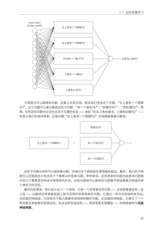


![2.2. 关于代价函数的两个假设
我们的作⽤函数是 f(x) = x2,那么向量化的 f 的函数作⽤就起到下⾯的效果:
f
([
2
3
])
=
[
f(2)
f(3)
]
=
[
4
9
]
(24)
也就是说,向量化的 f 仅仅是对向量的每个元素进⾏了平⽅运算。
了解了这些表⽰,⽅程 (23) 就可以写成下⾯这种美妙⽽简洁的向量形式了:
al
= σ(wl
al−1
+ bl
) (25)
这个表达式给出了⼀种更加全局的思考每层的激活值和前⼀层激活值的关联⽅式:我们仅仅
⽤权重矩阵作⽤在激活值上,然后加上⼀个偏置向量,最后作⽤ σ 函数 1。这种全局的观点相⽐
神经元层⾯的观点常常更加简明(没有更多的索引下标了!)。把它看做是在保留清晰认识的前
提下逃离下标困境的⽅法。在实践中,表达式同样很有⽤,因为⼤多数矩阵库提供了实现矩阵
乘法、向量加法和向量化的快速⽅法。实际上,上⼀章的代码其实已经隐式使⽤了这种表达式
来计算⽹络⾏为。
在使⽤⽅程 (25) 计算 al 的过程中,我们计算了中间量 zl ≡ wlal−1 + bl。这个量其实是
⾮常有⽤的:我们称 zl 为 l 层神经元的带权输⼊。在本章后⾯,我们会充分利⽤带权输⼊
zl。⽅程 (25) 有时候会以带权输⼊的形式写作 al = σ(zl)。同样要指出的是 zl 的每个元素是
zl
j =
∑
k wl
jkal−1
k + bl
j,其实 zl
j 就是第 l 层第 j 个神经元的激活函数的带权输⼊。
2.2 关于代价函数的两个假设
反向传播的⽬标是计算代价函数 C 分别关于 w 和 b 的偏导数 ∂C/∂w 和 ∂C/∂b。为了让反向
传播可⾏,我们需要做出关于代价函数的两个主要假设。在给出这两个假设之前,我们先看看
具体的⼀个代价函数。我们会使⽤上⼀章使⽤的⼆次代价函数(参⻅⽅程 (6))。按照上⼀节给
出的表⽰,⼆次代价函数有下列形式:
C =
1
2n
∑
x
∥y(x) − aL
(x)∥2
(26)
其中 n 是训练样本的总数;求和运算遍历了每个训练样本 x;y = y(x) 是对应的⽬标输出;L 表
⽰⽹络的层数;aL = aL(x) 是当输⼊是 x 时的⽹络输出的激活值向量。
好了,为了应⽤反向传播,我们需要对代价函数 C 做出什么样的前提假设呢?第⼀个假设就
是代价函数可以被写成⼀个在每个训练样本 x 上的代价函数 Cx 的均值 C = 1
n
∑
x Cx。这是关
于⼆次代价函数的例⼦,其中对每个独⽴的训练样本其代价是 Cx = 1
2 ||y − aL||2。这个假设对书
中提到的其他任何⼀个代价函数也都是必须满⾜的。
需要这个假设的原因是反向传播实际上是对⼀个独⽴的训练样本计算了 ∂Cx/∂w 和 ∂Cx/∂b。
然后我们通过在所有训练样本上进⾏平均化获得 ∂C/∂w 和 ∂C/∂b。实际上,有了这个假设,我
们会认为训练样本 x 已经被固定住了,丢掉了其下标,将代价函数 Cx 看做 C。最终我们会把下
标加上,现在为了简化表⽰其实没有这个必要。
第⼆个假设就是代价可以写成神经⽹络输出的函数:
1
其实,这就是让我们使⽤之前的矩阵下标 wl
jk 表⽰的初因。如果我们使⽤ j 来索引输⼊神经元,k 索引输出神经
元,那么在⽅程 (25) 中我们需要将这⾥的矩阵换做其转置。这是⼀个⼩的改变,但是令⼈困惑,这会使得我们⽆法
⾃然地讲出(思考)“应⽤权重矩阵到激活值上”这样的简单的表达。
36](https://image.slidesharecdn.com/nndl-ebook5-160513104940/85/slide-46-320.jpg)
![2.3. Hadamard 乘积,s ⊙ t
cost C = C(aL
)
aL
2
aL
1
例如,⼆次代价函数满⾜这个要求,因为对于⼀个单独的训练样本 x 其⼆次代价函数可以写
作:
C =
1
2
∥y − aL
∥2
=
1
2
∑
j
(yj − aL
j )2
(27)
这是输出的激活值的函数。当然,这个代价函数同样还依赖于⽬标输出 y,你可能奇怪为什么我
们不把代价也看作⼀个 y 的函数。记住,输⼊的训练样本 x 是固定的,所以输出 y 同样是⼀个
固定的参数。尤其是它并不是可以随意通过改变权重和偏置来改变的,也就是说,这不是神经
⽹络学习的对象。所以,将 C 看成仅有输出激活值 aL 的函数才是合理的,⽽ y 仅仅是帮助定义
函数的参数⽽已。
2.3 Hadamard 乘积,s ⊙ t
反向传播算法基于常规的线性代数运算 —— 诸如向量加法,向量矩阵乘法等。但是有⼀个运
算不⼤常⻅。特别地,假设 s 和 t 是两个同样维度的向量。那么我们使⽤ s ⊙ t 来表⽰按元素的
乘积。所以 s ⊙ t 的元素就是 (s ⊙ t)j = sjtj。给个例⼦,
[
1
2
]
⊙
[
3
4
]
=
[
1 ∗ 3
2 ∗ 4
]
=
[
3
8
]
(28)
这种类型的按元素乘法有时候被称为 Hadamard 乘积,或者 Schur 乘积。我们这⾥取前者。
好的矩阵库通常会提供 Hadamard 乘积的快速实现,在实现反向传播的时候⽤起来很⽅便。
2.4 反向传播的四个基本⽅程
反向传播其实是对权重和偏置变化影响代价函数过程的理解。最终极的含义其实就是计算偏
导数 ∂C/∂wl
jk 和 ∂C/∂bl
j。但是为了计算这些值,我们⾸先引⼊⼀个中间量,δl
j,这个我们称为
在 lth 层第 jth 个神经元上的误差。
反向传播将给出计算误差 δl
j 的流程,然后将其关联到计算 ∂C/∂wl
jk 和 ∂C/∂bl
j 上。
为了理解误差是如何定义的,假设在神经⽹络上有⼀个调⽪⻤:
37](https://image.slidesharecdn.com/nndl-ebook5-160513104940/85/slide-47-320.jpg)


![2.7. 代码
class Network(object):
...
def update_mini_batch(self, mini_batch, eta):
"""Update the network's weights and biases by applying
gradient descent using backpropagation to a single mini batch.
The "mini_batch" is a list of tuples "(x, y)", and "eta"
is the learning rate."""
nabla_b = [np.zeros(b.shape) for b in self.biases]
nabla_w = [np.zeros(w.shape) for w in self.weights]
for x, y in mini_batch:
delta_nabla_b, delta_nabla_w = self.backprop(x, y)
nabla_b = [nb+dnb for nb, dnb in zip(nabla_b, delta_nabla_b)]
nabla_w = [nw+dnw for nw, dnw in zip(nabla_w, delta_nabla_w)]
self.weights = [w-(eta/len(mini_batch))*nw
for w, nw in zip(self.weights, nabla_w)]
self.biases = [b-(eta/len(mini_batch))*nb
for b, nb in zip(self.biases, nabla_b)]
主要⼯作其实是在 delta_nabla_b,delta_nabla_w = self.backprop(x, y) 这⾥完成的,调⽤了
backprop ⽅法计算出了偏导数,∂Cx/∂bl
j 和 ∂Cx/∂wl
jk。backprop ⽅法跟上⼀节的算法基本⼀致。
这⾥只有个⼩⼩的差异 —— 我们使⽤⼀个略微不同的⽅式来索引神经⽹络的层。这个改变其实
是为了 Python 的特性 —— 负值索引的使⽤能够让我们从列表的最后往前遍历,如 l[-3] 其实是
列表中的倒数第三个元素。下⾯ backprop 的代码,和⼀些帮助函数⼀起,被⽤于计算 σ、导数 σ′
及代价函数的导数。所以理解了这些,我们就完全可以掌握所有的代码了。如果某些东西让你
困惑,你可能需要参考代码的原始描述(以及完整清单)。
class Network(object):
...
def backprop(self, x, y):
"""Return a tuple "(nabla_b, nabla_w)" representing the
gradient for the cost function C_x. "nabla_b" and
"nabla_w" are layer-by-layer lists of numpy arrays, similar
to "self.biases" and "self.weights"."""
nabla_b = [np.zeros(b.shape) for b in self.biases]
nabla_w = [np.zeros(w.shape) for w in self.weights]
# feedforward
activation = x
activations = [x] # list to store all the activations, layer by layer
zs = [] # list to store all the z vectors, layer by layer
for b, w in zip(self.biases, self.weights):
z = np.dot(w, activation)+b
zs.append(z)
activation = sigmoid(z)
activations.append(activation)
# backward pass
delta = self.cost_derivative(activations[-1], y) *
sigmoid_prime(zs[-1])
nabla_b[-1] = delta
nabla_w[-1] = np.dot(delta, activations[-2].transpose())
# Note that the variable l in the loop below is used a little
# differently to the notation in Chapter 2 of the book. Here,
# l = 1 means the last layer of neurons, l = 2 is the
# second-last layer, and so on. It's a renumbering of the
# scheme in the book, used here to take advantage of the fact
# that Python can use negative indices in lists.
for l in xrange(2, self.num_layers):
z = zs[-l]
sp = sigmoid_prime(z)
delta = np.dot(self.weights[-l+1].transpose(), delta) * sp
44](https://image.slidesharecdn.com/nndl-ebook5-160513104940/85/slide-54-320.jpg)
![2.8. 在哪种层⾯上,反向传播是快速的算法?
nabla_b[-l] = delta
nabla_w[-l] = np.dot(delta, activations[-l-1].transpose())
return (nabla_b, nabla_w)
...
def cost_derivative(self, output_activations, y):
"""Return the vector of partial derivatives partial C_x /
partial a for the output activations."""
return (output_activations-y)
def sigmoid(z):
"""The sigmoid function."""
return 1.0/(1.0+np.exp(-z))
def sigmoid_prime(z):
"""Derivative of the sigmoid function."""
return sigmoid(z)*(1-sigmoid(z))
问题
• 在⼀个⼩批量数据上的反向传播的全矩阵⽅法 我们对于随机梯度下降的实现是对⼀
个⼩批量数据中的训练样本进⾏遍历。所以也可以更改反向传播算法使得它同时对
⼀个⼩批量数据中的所有样本进⾏梯度计算。这个想法其实就是我们可以⽤⼀个矩阵
X = [x1, x2, ..., xm],其中每列就是在⼩批量数据中的向量,⽽不是单个的输⼊向量,x。
我们通过乘权重矩阵,加上对应的偏置进⾏前向传播,在所有地⽅应⽤ S 型函数。然后按
照类似的过程进⾏反向传播。请显式写出这种⽅法下的伪代码。更改 network.py 来实现这
个⽅案。这样做的好处其实利⽤到了现代的线性代数库。所以,这会⽐在⼩批量数据上进
⾏遍历要运⾏得更快(在我的笔记本电脑上,在 MNIST 分类问题上,我相较于上⼀章的
实现获得了 2 倍的速度提升)。在实际应⽤中,所有靠谱的反向传播的库都是⽤了类似的
基于矩阵或者其变化形式来实现的。
2.8 在哪种层⾯上,反向传播是快速的算法?
在哪种层⾯上,反向传播是快速的算法?为了回答这个问题,⾸先考虑另⼀个计算梯度的⽅
法。就当我们回到上世界 50、60 年代的神经⽹络研究。假设你是世界上⾸个考虑使⽤梯度下降
⽅法学习的那位!为了让⾃⼰的想法可⾏,就必须找出计算代价函数梯度的⽅法。想想⾃⼰学到
的微积分,决定试试看链式法则来计算梯度。但玩了⼀会后,就发现代数式看起来⾮常复杂,然
后就退缩了。所以就试着找另外的⽅式。你决定仅仅把代价看做权重的函数 C = C(w)(我们⻢
上会回到偏置)。你给这些权重 w1, w2, . . . 进⾏编号,期望计算某些权重 wj 的偏导数 ∂C/∂wj。
⽽⼀种近似的⽅法就是下⾯这种:
∂C
∂wj
≈
C(w + ϵej) − C(w)
ϵ
(46)
其中 ϵ > 0 是⼀个很⼩的正数,⽽ ej 是在第 j 个⽅向上的单位向量。换句话说,我们可以通
过计算两个接近相同的 wj 值的代价 C 来估计 ∂C/∂wj,然后应⽤公式 (46)。同样⽅法也可以⽤
来计算 ∂C/∂b。
45](https://image.slidesharecdn.com/nndl-ebook5-160513104940/85/slide-55-320.jpg)


![3.1. 交叉熵代价函数
其中我已经将 x = 1 和 y = 0 代⼊了。为了理解这些表达式的⾏为,让我们仔细看 σ′(z) 这
⼀项。⾸先回忆⼀下 σ 函数图像:
−4 −3 −2 −1 0 1 2 3 4
0.0
0.2
0.4
0.6
0.8
1.0
Z
sigmoid function
我们可以从这幅图看出,当神经元的输出接近 1 的时候,曲线变得相当平,所以 σ′(z) 就很
⼩了。⽅程 (55) 和 (56) 也告诉我们 ∂C/∂w 和 ∂C/∂b 会⾮常⼩。这其实就是学习缓慢的原因所
在。⽽且,我们后⾯也会提到,这种学习速度下降的原因实际上也是更加⼀般的神经⽹络学习
缓慢的原因,并不仅仅是在这个特例中特有的。
3.1.1 引⼊交叉熵代价函数
那么我们如何解决这个问题呢?研究表明,我们可以通过使⽤交叉熵代价函数来替换⼆次代
价函数。为了理解什么是交叉熵,我们稍微改变⼀下之前的简单例⼦。假设,我们现在要训练
⼀个包含若⼲输⼊变量的的神经元,x1, x2, . . . 对应的权重为 w1, w2, . . . 和偏置 b:
bx2
x1
x3
a = σ(z)
w1
w2
w3
神经元的输出就是 a = σ(z),其中 z =
∑
j wjxj + b 是输⼊的带权和。我们如下定义这个神
经元的交叉熵代价函数:
C = −
1
n
∑
x
[y ln a + (1 − y) ln(1 − a)] (57)
其中 n 是训练数据的总数,求和是在所有的训练输⼊ x 上进⾏的,y 是对应的⽬标输出。
表达式 (57) 是否解决学习缓慢的问题并不明显。实际上,甚⾄将这个定义看做是代价函数也
不是显⽽易⻅的!在解决学习缓慢前,我们来看看交叉熵为何能够解释成⼀个代价函数。
将交叉熵看做是代价函数有两点原因。第⼀,它是⾮负的,C > 0。可以看出:(a)(57) 中的
求和中的所有独⽴的项都是负数的,因为对数函数的定义域是 (0, 1);(b)求和前⾯有⼀个负号。
第⼆,如果对于所有的训练输⼊ x,神经元实际的输出接近⽬标值,那么交叉熵将接近 01。
假设在这个例⼦中,y = 0 ⽽ a ≈ 0。这是我们想到得到的结果。我们看到公式 (57) 中第⼀个项
1
为了证明它我需要假设⽬标输出 y 都是 0 或 1。这通常是解决分类问题的情况,例如,当计算布尔函数时。要了
解当我们不做这个假设时会发⽣什么,看看在本节结束时的练习。
54](https://image.slidesharecdn.com/nndl-ebook5-160513104940/85/slide-64-320.jpg)


![3.1. 交叉熵代价函数
值。那么我们定义交叉熵如下
C = −
1
n
∑
x
∑
j
[
yj ln aL
j + (1 − yj) ln(1 − aL
j )
]
(63)
除了这⾥需要对所有输出神经元进⾏求和
∑
j 外,这个其实和我们早前的公式 (57) 是⼀样
的。这⾥不会给出⼀个推算的过程,但需要说明的时使⽤公式 (63) 确实会在很多的神经⽹络中
避免学习的缓慢。如果你感兴趣,你可以尝试⼀下下⾯问题的推导。
那么我们应该在什么时候⽤交叉熵来替换⼆次代价函数?实际上,如果在输出神经元是 S 型
神经元时,交叉熵⼀般都是更好的选择。为什么?考虑⼀下我们初始化⽹络的权重和偏置时时
候通常使⽤某种随机⽅法。可能会发⽣这样的情况,这些初始选择会对某些训练输⼊误差相当
明显 —— ⽐如说,⽬标输出是 1,⽽实际值是 0,或者完全反过来。如果我们使⽤⼆次代价函数,
那么这就会导致学习速度的下降。它并不会完全终⽌学习的过程,因为这些权重会持续从其他
的样本中进⾏学习,但是显然这不是我们想要的效果。
练习
• ⼀个⼩问题就是刚接触交叉熵时,很难⼀下⼦记住那些诸如 y 和 a 的表达式对应的⻆⾊。
⼜⽐如说,表达式的正确形式是 −[y ln a+(1−y) ln(1−a)] 还是 −[a ln y +(1−a) ln(1−y)]。
在 y = 0 或者 1 的时候第⼆个表达式的结果怎样?这个问题会困扰第⼀个表达式吗?为什
么?
• 在对单个神经元讨论中,我们指出如果对所有的训练数据有 σ(z) ≈ y,交叉熵会很⼩。这
个论断其实是和 y 只是等于 1 或者 0 有关。这在分类问题⼀般是可⾏的,但是对其他的
问题(如回归问题)y 可以取 0 和 1 之间的中间值的。证明,交叉熵对所有训练输⼊在
σ(z) = y 时仍然是最⼩化的。此时交叉熵的表⽰是:
C = −
1
n
∑
x
[y ln y + (1 − y) ln(1 − y)] (64)
⽽其中 −[y ln y + (1 − y) ln(1 − y)] 有时候被称为⼆元熵。
问题
• 多层多神经元⽹络 ⽤上⼀章的定义符号,证明对⼆次代价函数,关于输出层的权重的偏
导数为
∂C
∂wL
jk
=
1
n
∑
x
aL−1
k (aL
j − yj)σ′
(zL
j ) (65)
项 σ′(zL
j ) 会在⼀个输出神经元困在错误值时导致学习速度的下降。证明对于交叉熵代价函
数,针对⼀个训练样本 x 的输出误差 δL 为
δL
= aL
− y (66)
使⽤这个表达式来证明关于输出层的权重的偏导数为
∂C
∂wL
jk
=
1
n
∑
x
aL−1
k (aL
j − yj) (67)
59](https://image.slidesharecdn.com/nndl-ebook5-160513104940/85/slide-69-320.jpg)
![3.1. 交叉熵代价函数
这⾥ σ′(zL
j ) 就消失了,所以交叉熵避免了学习缓慢的问题,不仅仅是在⼀个神经元上,⽽
且在多层多元⽹络上都起作⽤。这个分析过程稍作变化对偏置也是⼀样的。如果你对这个
还不确定,那么请仔细研读⼀下前⾯的分析。
• 在输出层使⽤线性神经元时使⽤⼆次代价函数 假设我们有⼀个多层多神经元⽹络,最终
输出层的神经元都是线性神经元,输出不再是 S 型函数作⽤的结果,⽽是 aL
j = zL
j 。证明
如果我们使⽤⼆次代价函数,那么对单个训练样本 x 的输出误差就是
δL
= aL
− y (68)
类似于前⼀个问题,使⽤这个表达式来证明关于输出层的权重和偏置的偏导数为
∂C
∂wL
jk
=
1
n
∑
x
aL−1
k (aL
j − yj) (69)
∂C
∂bL
j
=
1
n
∑
x
(aL
j − yj) (70)
这表明如果输出神经元是线性的那么⼆次代价函数不再会导致学习速度下降的问题。在此
情形下,⼆次代价函数就是⼀种合适的选择。
3.1.2 使⽤交叉熵来对 MNIST 数字进⾏分类
交叉熵很容易作为使⽤梯度下降和反向传播⽅式进⾏模型学习的⼀部分来实现。我们将会这
⼀章的后⾯进⾏对 前⾯的程序 network.py 的改进。新的程序写在 network2.py 中,不仅使⽤了
交叉熵,还有本章中介绍的其他的技术2。现在我们看看新的程序在进⾏ MNIST 数字分类问题
上的表现。如在第⼀章中那样,我们会使⽤⼀个包含 30 个隐藏元的⽹络,⽽⼩批量数据的⼤
⼩也设置为 10。我们将学习速率设置为 η = 0.5 3 然后训练 30 个迭代期。network2.py 的接⼝和
network.py 稍微不同,但是过程还是很清楚的。你可以使⽤如 help(network2.Network.SGD) 这样的
命令来查看 network2.py 的接⼝⽂档。
>>> import mnist_loader
>>> training_data, validation_data, test_data =
... mnist_loader.load_data_wrapper()
>>> import network2
>>> net = network2.Network([784, 30, 10], cost=network2.CrossEntropyCost)
>>> net.large_weight_initializer()
>>> net.SGD(training_data, 30, 10, 0.5, evaluation_data=test_data,
... monitor_evaluation_accuracy=True)
注意看下,net.large_weight_initializer() 命令使⽤和第⼀章介绍的同样的⽅式来进⾏权重
和偏置的初始化。我们需要运⾏这个命令,是因为我们要在这⼀章的后⾯才改变默认的权重初
始化命令。运⾏上⾯的代码我们得到了⼀个 95.49% 准确率的⽹络。这跟我们在第⼀章中使⽤⼆
次代价函数得到的结果相当接近了,95.42%。
2
代码可从 GitHub 获取。
3
在第⼀章⾥我们⽤了⼆次代价和 η = 3.0 的学习速率。上⾯已经讨论过,准确地说出当代价函数改变时⽤“相同
的”学习速率意味什么,这是不可能的。对于两种代价函数,在给出其它超参数的选择后,我都做了实验来找出⼀个接
近优化性能的学习速率,顺便提⼀下,有⼀个⾮常粗略的将交叉熵和⼆次代价的学习速率联系起来的推导。正如我们
之前看到的,⼆次代价的梯度项中有⼀个额外的 σ′
= σ(1−σ)。假设我们把这按照 σ 的值平均,
∫ 1
0
dσσ(1−σ) = 1/6。
我们(⾮常粗略地)看到⼆次代价对于相同的学习速率,以平均慢 6 倍的速度进⾏学习。这提⽰我们⼀个合理的起点
是把⼆次代价的学习速率除以 6。当然,这个理由⾮常不严谨,不应被认真对待。不过,有时候这是个有⽤的起点。
60](https://image.slidesharecdn.com/nndl-ebook5-160513104940/85/slide-70-320.jpg)

![3.1. 交叉熵代价函数
使⽤ σ′(z) = σ(z)(1 − σ(z)) = a(1 − a),上个等式就变成
∂C
∂b
=
∂C
∂a
a(1 − a) (74)
对⽐等式 (72),我们有
∂C
∂a
=
a − y
a(1 − a)
(75)
对此⽅程关于 a 进⾏积分,得到
C = −[y ln a + (1 − y) ln(1 − a)] + constant (76)
其中 constant 是积分常量。这是⼀个单独的训练样本 x 对代价函数的贡献。为了得到整个的代
价函数,我们需要对所有的训练样本进⾏平均,得到了
C = −
1
n
∑
x
[y ln a + (1 − y) ln(1 − a)] + constant (77)
⽽这⾥的常量就是所有单独的常量的平均。所以我们看到⽅程 (71) 和 (72) 唯⼀确定了交叉熵的
形式,并加上了⼀个常量的项。这个交叉熵并不是凭空产⽣的。⽽是⼀种我们以⾃然和简单的
⽅法获得的结果。
那么交叉熵直觉含义⼜是什么?我们如何看待它?深⼊解释这⼀点会将我们带到⼀个不⼤愿
意讨论的领域。然⽽,还是值得提⼀下,有⼀种源⾃信息论的解释交叉熵的标准⽅式。粗略地
说,交叉熵是“不确定性”的⼀种度量。特别地,我们的神经元想要计算函数 x → y = y(x)。但
是,它⽤函数 x → a = a(x) 进⾏了替换。假设我们将 a 想象成我们神经元估计为 y = 1 的概率,
⽽ 1 − a 则是 y = 0 的概率。那么交叉熵衡量我们学习到 y 的正确值的平均起来的不确定性。如
果输出我们期望的结果,不确定性就会⼩⼀点;反之,不确定性就⼤⼀些。当然,我这⾥没有严
格地给出“不确定性”到底意味着什么,所以看起来像在夸夸奇谈。但是实际上,在信息论中有
⼀种准确的⽅式来定义不确定性究竟是什么。不过,我也不清楚在⽹络上,哪⾥有好的、短⼩
的、包含有对这个主题的讨论。但如果你要深⼊了解的话,维基百科包含⼀个简短的总结,这
会指引你正确地探索这个领域。⽽更加细节的内容,你们可以阅读 Cover and Thomas 的第五章
涉及 Kraft 不等式的有关信息论的内容。
问题
• 我们已经深⼊讨论了使⽤⼆次代价函数的⽹络中在输出神经元饱和时候学习缓慢的问题,
另⼀个可能会影响学习的因素就是在⽅程 (61) 中的 xj 项。由于此项,当输⼊ xj 接近 0 时,
对应的权重 wj 会学习得相当缓慢。解释为何不可以通过改变代价函数来消除 xj 项的影响。
3.1.4 柔性最⼤值
本章,我们⼤多数情况会使⽤交叉熵来解决学习缓慢的问题。但是,我希望简要介绍⼀下另
⼀种解决这个问题的⽅法,基于柔性最⼤值(softmax)神经元层。我们不会实际在剩下的章节
中使⽤柔性最⼤值层,所以你如果赶时间,就可以跳到下⼀个⼩节了。不过,柔性最⼤值仍然
有其重要价值,⼀⽅⾯它本⾝很有趣,另⼀⽅⾯,因为我们会在第六章在对深度神经⽹络的讨
论中使⽤柔性最⼤值层。
62](https://image.slidesharecdn.com/nndl-ebook5-160513104940/85/slide-72-320.jpg)


![3.2. 过度拟合和规范化
3.2 过度拟合和规范化
诺⻉尔奖获得者,物理学家恩⾥科·费⽶有⼀次被问到他对⼀些同僚提出的⼀个数学模型的
意⻅,这个数学模型尝试解决⼀个重要的未解决的物理难题。模型和实验⾮常匹配,但是费⽶却
对其产⽣了怀疑。他问模型中需要设置的⾃由参数有多少个。答案是“4”。费⽶回答道6:“我记
得我的朋友约翰·冯·诺伊曼过去常说,有四个参数,我可以模拟⼀头⼤象,⽽有五个参数,我
还能让他卷⿐⼦。”
这⾥,其实是说拥有⼤量的⾃由参数的模型能够描述特别神奇的现象。即使这样的模型能够
很好的拟合已有的数据,但并不表⽰是⼀个好模型。因为这可能只是因为模型中⾜够的⾃由度
使得它可以描述⼏乎所有给定⼤⼩的数据集,⽽不需要真正洞察现象的本质。所以发⽣这种情
形时,模型对已有的数据会表现的很好,但是对新的数据很难泛化。对⼀个模型真正的测验就
是它对没有⻅过的场景的预测能⼒。
费⽶和冯·诺伊曼对有四个参数的模型就开始怀疑了。我们⽤来对 MNIST 数字分类的 30 个
隐藏神经元神经⽹络拥有将近 24,000 个参数!当然很多。我们有 100 个隐藏元的⽹络拥有将近
80,000 个参数,⽽⽬前最先进的深度神经⽹络包含百万级或者⼗亿级的参数。我们应当信赖这
些结果么?
让我们通过构造⼀个⽹络泛化能⼒很差的例⼦使这个问题更清晰。我们的⽹络有 30 个隐藏
神经元,共 23,860 个参数。但是我们不会使⽤所有 50,000 幅 MNIST 训练图像。相反,我们只
使⽤前 1,000 幅图像。使⽤这个受限的集合,会让泛化的问题突显。我们按照之前同样的⽅式,
使⽤交叉熵代价函数,学习速率设置为 η = 0.5 ⽽⼩批量数据⼤⼩设置为 10。不过这⾥我们要训
练 400 个迭代期,⽐前⾯的要多⼀些,因为我们只⽤了少量的训练样本。我们现在使⽤ network2
来研究代价函数改变的情况:
>>> import mnist_loader
>>> training_data, validation_data, test_data =
... mnist_loader.load_data_wrapper()
>>> import network2
>>> net = network2.Network([784, 30, 10], cost=network2.CrossEntropyCost)
>>> net.large_weight_initializer()
>>> net.SGD(training_data[:1000], 400, 10, 0.5, evaluation_data=test_data,
... monitor_evaluation_accuracy=True, monitor_training_cost=True)
使⽤上⾯的结果,我们可以画出当⽹络学习时代价变化的情况7:
6
这个引⽤的故事来⾃⼀篇 Freeman Dyson 所写的引⼈⼊胜的⽂章。他是提出这个有瑕疵的模型的⼈之⼀。⼀个
关于四个参数模拟⼤象的例⼦可以在这⾥找到。
7
这个图形以及接下来的四个由程序 overfitting.py ⽣成。
67](https://image.slidesharecdn.com/nndl-ebook5-160513104940/85/slide-77-320.jpg)


![3.2. 过度拟合和规范化
如你所⻅,测试集和训练集上的准确率相⽐我们使⽤ 1, 000 个训练数据时相差更⼩。特别地,
在训练数据上的最佳的分类准确率 97.86% 只⽐测试集上的 95.33% 准确率⾼了 1.53%。⽽之前
的例⼦中,这个差距是 17.73%!过度拟合仍然发⽣了,但是已经减轻了不少。我们的⽹络从训
练数据上更好地泛化到了测试数据上。⼀般来说,最好的降低过度拟合的⽅式之⼀就是增加训
练样本的量。有了⾜够的训练数据,就算是⼀个规模⾮常⼤的⽹络也不⼤容易过度拟合。不幸
的是,训练数据其实是很难或者很昂贵的资源,所以这不是⼀种太切实际的选择。
3.2.1 规范化
增加训练样本的数量是⼀种减轻过度拟合的⽅法。还有其他的⼀下⽅法能够减轻过度拟合的
程度吗?⼀种可⾏的⽅式就是降低⽹络的规模。然⽽,⼤的⽹络拥有⼀种⽐⼩⽹络更强的潜⼒,
所以这⾥存在⼀种应⽤冗余性的选项。
幸运的是,还有其他的技术能够缓解过度拟合,即使我们只有⼀个固定的⽹络和固定的训练
集合。这种技术就是规范化。本节,我会给出⼀种最为常⽤的规范化⼿段 —— 有时候被称为权
重衰减(weight decay)或者 L2 规范化。L2 规范化的想法是增加⼀个额外的项到代价函数上,
这个项叫做规范化项。下⾯是规范化的交叉熵:
C = −
1
n
∑
xj
[
yj ln aL
j + (1 − yj) ln(1 − aL
j )
]
+
λ
2n
∑
w
w2
(85)
其中第⼀个项就是常规的交叉熵的表达式。第⼆个现在加⼊的就是所有权重的平⽅的和。然
后使⽤⼀个因⼦ λ/2n 进⾏量化调整,其中 λ > 0 可以称为规范化参数,⽽ n 就是训练集合的⼤
⼩。我们会在后⾯讨论 λ 的选择策略。需要注意的是,规范化项⾥⾯并不包含偏置。这点我们
后⾯也会在讲述。
当然,对其他的代价函数也可以进⾏规范化,例如⼆次代价函数。类似的规范化的形式如下:
C =
1
2n
∑
x
∥y − aL
∥2
+
λ
2n
∑
w
w2
(86)
两者都可以写成这样:
C = C0 +
λ
2n
∑
w
w2
(87)
71](https://image.slidesharecdn.com/nndl-ebook5-160513104940/85/slide-81-320.jpg)

![3.2. 过度拟合和规范化
让我们看看规范化给⽹络带来的性能提升吧。这⾥还会使⽤有 30 个隐藏神经元、⼩批量数
据 ⼤⼩为 10,学习速率为 0.5,使⽤交叉熵的神经⽹络。然⽽,这次我们会使⽤规范化参数为
λ = 0.1。注意在代码中,我们使⽤的变量名字为 lmbda,这是因为在 Python 中 lambda 是关键字,
有着不相关的含义。我也会再次使⽤ test_data,⽽不是 validation_data。不过严格地讲,我们应
当使⽤ validation_data 的,因为前⾯已经讲过了。这⾥我这样做,是因为这会让结果和⾮规范化
的结果对⽐起来效果更加直接。你可以轻松地调整为 validation_data,你会发现有相似的结果。
>>> import mnist_loader
>>> training_data, validation_data, test_data =
... mnist_loader.load_data_wrapper()
>>> import network2
>>> net = network2.Network([784, 30, 10], cost=network2.CrossEntropyCost)
>>> net.large_weight_initializer()
>>> net.SGD(training_data[:1000], 400, 10, 0.5,
... evaluation_data=test_data, lmbda = 0.1,
... monitor_evaluation_cost=True, monitor_evaluation_accuracy=True,
... monitor_training_cost=True, monitor_training_accuracy=True)
训练集上的代价函数持续下降,和前⾯⽆规范化的情况⼀样的规律9:
200 250 300 350 400
Epoch
0.10
0.12
0.14
0.16
0.18
0.20
0.22
0.24
0.26 Cost on the training data
但是这次测试集上的准确率在整个 400 迭代期内持续增加:
200 250 300 350 400
Epoch
85.8
86.0
86.2
86.4
86.6
86.8
87.0
87.2
Accuracy (%) on the test data
9
这个以及下⼀个图像由程序 overfitting.py ⽣成。
73](https://image.slidesharecdn.com/nndl-ebook5-160513104940/85/slide-83-320.jpg)
![3.2. 过度拟合和规范化
显然,规范化的使⽤能够解决过度拟合的问题。⽽且,准确率相当⾼了,最⾼处达到了 87.1%,
相较于之前的 82.27%。因此,我们⼏乎可以确信在 400 迭代期之后持续训练会有更加好的结果。
看起来,经实践检验,规范化让⽹络具有更好的泛化能⼒,显著地减轻了过度拟合的影响。
如果我们摆脱⼈为的仅⽤ 1,000 个训练图像的环境,转⽽⽤所有 50,000 图像的训练集,会发
⽣什么?当然,我们之前已经看到过度拟合在⼤规模的数据上其实不是那么明显了。那规范化
能不能起到相应的作⽤呢?保持超参数和之前⼀样,30 迭代期, 学习速率为 0.5, ⼩批量数据⼤⼩
为 10。不过我们这⾥需要改变规范化参数。原因在于训练数据的⼤⼩已经从 n = 1, 000 改成了
n = 50, 000,这个会改变权重衰减因⼦ 1 − ηλ
n 。如果我们持续使⽤ λ = 0.1 就会产⽣很⼩的权重
衰减,因此就将规范化的效果降低很多。我们通过修改为 λ = 5.0 来补偿这种下降。
好了,来训练⽹络,重新初始化权重:
>>> net.large_weight_initializer()
>>> net.SGD(training_data, 30, 10, 0.5,
... evaluation_data=test_data, lmbda = 5.0,
... monitor_evaluation_accuracy=True, monitor_training_accuracy=True)
我们得到:
这个结果很不错。第⼀,我们在测试集上的分类准确率在使⽤规范化后有了提升,从 95.49%
到 96.49%。这是个很⼤的进步。第⼆,我们可以看到在训练数据和测试数据上的结果之间的差
距也更⼩了。这仍然是⼀个⼤的差距,不过我们已经显著得到了本质上的降低过度拟合的进步。
最后,我们看看在使⽤ 100 个隐藏神经元和规范化参数为 λ = 5.0 相应的测试分类准确率。
我不会给出详细分析,纯粹为了好玩,来看看我们使⽤⼀些技巧(交叉熵函数和 L2 规范化)能
够达到多⾼的准确率。
>>> net = network2.Network([784, 100, 10], cost=network2.CrossEntropyCost)
>>> net.large_weight_initializer()
>>> net.SGD(training_data, 30, 10, 0.5, lmbda=5.0,
... evaluation_data=validation_data,
... monitor_evaluation_accuracy=True)
最终在验证集上的准确率达到了 97.92%。这是⽐ 30 个隐藏元的较⼤⻜跃。实际上,稍微改
变⼀点,60 迭代期 η = 0.1 和 λ = 5.0。我们就突破了 98%,达到了 98.04% 的分类准确率。对
于 152 ⾏代码这个效果还真不错!
我已经把规范化描述为⼀种减轻过度拟合和提⾼分类准确率的⽅法。实际上,这不是仅有的
好处。实践表明,在使⽤不同的(随机)权重初始化进⾏多次 MNIST ⽹络训练的时候,我发现
74](https://image.slidesharecdn.com/nndl-ebook5-160513104940/85/slide-84-320.jpg)


![3.3. 权重初始化
“`python
>>> import mnist_loader
>>> training_data, validation_data, test_data =
... mnist_loader.load_data_wrapper()
>>> import network2
>>> net = network2.Network([784, 30, 10], cost=network2.CrossEntropyCost)
>>> net.large_weight_initializer()
>>> net.SGD(training_data, 30, 10, 0.1, lmbda = 5.0,
... evaluation_data=validation_data,
... monitor_evaluation_accuracy=True)
我们也使⽤新⽅法来进⾏权重的初始化。这实际上还要更简单,因为 network2 默认⽅式就是
使⽤新的⽅法。这意味着我们可以丢掉上⾯的 net.large_weight_initializer() 调⽤:
>>> net = network2.Network([784, 30, 10], cost=network2.CrossEntropyCost)
>>> net.SGD(training_data, 30, 10, 0.1, lmbda = 5.0,
... evaluation_data=validation_data,
... monitor_evaluation_accuracy=True)
将结果⽤图展⽰出来21 ,我们得到:
0 5 10 15 20 25 30
Epoch
86
88
90
92
94
96
98
100 Classification accuracy
Old approach to weight initialization
New approach to weight initialization
两种情形下,我们在 96% 的准确率上重合了。最终的分类准确率⼏乎完全⼀样。但是新的初
始化技术带来了速度的提升。在第⼀种初始化⽅式的分类准确率在 87% 以下,⽽新的⽅法已经
⼏乎达到了 93%。看起来的情况就是我们新的关于权重初始化的⽅式将训练带到了⼀个新的境
界,让我们能够更加快速地得到好的结果。同样的情况在 100 个神经元的设定中也出现了:
21
⽤来⽣成这幅以及下⼀幅图形的程序是 weight_initialization.py 。
87](https://image.slidesharecdn.com/nndl-ebook5-160513104940/85/slide-97-320.jpg)

![3.4. 再看⼿写识别问题:代码
self.num_layers = len(sizes)
self.sizes = sizes
self.default_weight_initializer()
self.cost=cost
最开始⼏⾏⾥的 __init__ ⽅法的和 network.py 中⼀样,可以轻易弄懂。但是下⾯两⾏是新的,
我们需要知道他们到底做了什么。
我们先看看 default_weight_initializer ⽅法,使⽤了我们新式改进后的初始化权重⽅法。如
我们已经看到的,使⽤了均值为 0 ⽽标准差为 1/
√
n,n 为对应的输⼊连接个数。我们使⽤均值
为 0 ⽽标准差为 1 的⾼斯分布来初始化偏置。下⾯是代码:
def default_weight_initializer(self):
self.biases = [np.random.randn(y, 1) for y in self.sizes[1:]]
self.weights = [np.random.randn(y, x)/np.sqrt(x)
for x, y in zip(self.sizes[:-1], self.sizes[1:])]
为了理解这段代码,需要知道 np 就是进⾏线性代数运算的 Numpy 库。我们在程序的开头会
import Numpy。同样我们没有对第⼀层的神经元的偏置进⾏初始化。因为第⼀层其实是输⼊层,
所以不需要引⼊任何的偏置。我们在 network.py 中做了完全⼀样的事情。
作为 default_weight_initializer 的补充,我们同样包含了⼀个 large_weight_initializer ⽅法。
这个⽅法使⽤了第⼀章中的观点初始化了权重和偏置。代码也就仅仅是和 default_weight_initializer
差了⼀点点了:
def large_weight_initializer(self):
self.biases = [np.random.randn(y, 1) for y in self.sizes[1:]]
self.weights = [np.random.randn(y, x)
for x, y in zip(self.sizes[:-1], self.sizes[1:])]
我将 larger_weight_initializer ⽅法包含进来的原因也就是使得跟第⼀章的结果更容易⽐较。
我并没有考虑太多的推荐使⽤这个⽅法的实际情景。
初始化⽅法 __init__ 中的第⼆个新的东西就是我们初始化了 cost 属性。为了理解这个⼯作的
原理,让我们看⼀下⽤来表⽰交叉熵代价的类23:
class CrossEntropyCost(object):
@staticmethod
def fn(a, y):
return np.sum(np.nan_to_num(-y*np.log(a)-(1-y)*np.log(1-a)))
@staticmethod
def delta(z, a, y):
return (a-y)
让我们分解⼀下。第⼀个看到的是:即使使⽤的是交叉熵,数学上看,就是⼀个函数,这⾥我
们⽤ Python 的类⽽不是 Python 函数实现了它。为什么这样做呢?答案就是代价函数在我们的
⽹络中扮演了两种不同的⻆⾊。明显的⻆⾊就是代价是输出激活值 a 和⽬标输出 y 差距优劣的
度量。这个⻆⾊通过 CrossEntropyCost.fn ⽅法来扮演。(注意,np.nan_to_num 调⽤确保了 Numpy
正确处理接近 0 的对数值)但是代价函数其实还有另⼀个⻆⾊。回想第⼆章中运⾏反向传播算
法时,我们需要计算⽹络输出误差,δL。这种形式的输出误差依赖于代价函数的选择:不同的
23
如果你不熟悉 Python 的静态⽅法,你可以忽略 @staticmethod 装饰符,仅仅把 fn 和 delta 看作普通⽅法。如
果你想知道细节,所有的 @staticmethod 所做的是告诉 Python 解释器其随后的⽅法完全不依赖于对象。这就是为
什么 self 没有作为参数传⼊ fn 和 delta。
89](https://image.slidesharecdn.com/nndl-ebook5-160513104940/85/slide-99-320.jpg)
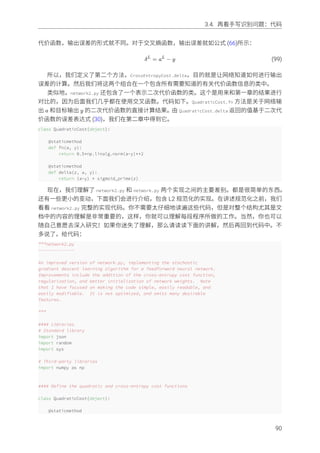
![3.4. 再看⼿写识别问题:代码
def fn(a, y):
"""Return the cost associated with an output ``a`` and desired output
``y``.
"""
return 0.5*np.linalg.norm(a-y)**2
@staticmethod
def delta(z, a, y):
"""Return the error delta from the output layer."""
return (a-y) * sigmoid_prime(z)
class CrossEntropyCost(object):
@staticmethod
def fn(a, y):
"""Return the cost associated with an output ``a`` and desired output
``y``. Note that np.nan_to_num is used to ensure numerical
stability. In particular, if both ``a`` and ``y`` have a 1.0
in the same slot, then the expression (1-y)*np.log(1-a)
returns nan. The np.nan_to_num ensures that that is converted
to the correct value (0.0).
"""
return np.sum(np.nan_to_num(-y*np.log(a)-(1-y)*np.log(1-a)))
@staticmethod
def delta(z, a, y):
"""Return the error delta from the output layer. Note that the
parameter ``z`` is not used by the method. It is included in
the method's parameters in order to make the interface
consistent with the delta method for other cost classes.
"""
return (a-y)
#### Main Network class
class Network(object):
def __init__(self, sizes, cost=CrossEntropyCost):
"""The list ``sizes`` contains the number of neurons in the respective
layers of the network. For example, if the list was [2, 3, 1]
then it would be a three-layer network, with the first layer
containing 2 neurons, the second layer 3 neurons, and the
third layer 1 neuron. The biases and weights for the network
are initialized randomly, using
``self.default_weight_initializer`` (see docstring for that
method).
"""
self.num_layers = len(sizes)
self.sizes = sizes
self.default_weight_initializer()
self.cost=cost
def default_weight_initializer(self):
"""Initialize each weight using a Gaussian distribution with mean 0
and standard deviation 1 over the square root of the number of
weights connecting to the same neuron. Initialize the biases
91](https://image.slidesharecdn.com/nndl-ebook5-160513104940/85/slide-101-320.jpg)
![3.4. 再看⼿写识别问题:代码
using a Gaussian distribution with mean 0 and standard
deviation 1.
Note that the first layer is assumed to be an input layer, and
by convention we won't set any biases for those neurons, since
biases are only ever used in computing the outputs from later
layers.
"""
self.biases = [np.random.randn(y, 1) for y in self.sizes[1:]]
self.weights = [np.random.randn(y, x)/np.sqrt(x)
for x, y in zip(self.sizes[:-1], self.sizes[1:])]
def large_weight_initializer(self):
"""Initialize the weights using a Gaussian distribution with mean 0
and standard deviation 1. Initialize the biases using a
Gaussian distribution with mean 0 and standard deviation 1.
Note that the first layer is assumed to be an input layer, and
by convention we won't set any biases for those neurons, since
biases are only ever used in computing the outputs from later
layers.
This weight and bias initializer uses the same approach as in
Chapter 1, and is included for purposes of comparison. It
will usually be better to use the default weight initializer
instead.
"""
self.biases = [np.random.randn(y, 1) for y in self.sizes[1:]]
self.weights = [np.random.randn(y, x)
for x, y in zip(self.sizes[:-1], self.sizes[1:])]
def feedforward(self, a):
"""Return the output of the network if ``a`` is input."""
for b, w in zip(self.biases, self.weights):
a = sigmoid(np.dot(w, a)+b)
return a
def SGD(self, training_data, epochs, mini_batch_size, eta,
lmbda = 0.0,
evaluation_data=None,
monitor_evaluation_cost=False,
monitor_evaluation_accuracy=False,
monitor_training_cost=False,
monitor_training_accuracy=False):
"""Train the neural network using mini-batch stochastic gradient
descent. The ``training_data`` is a list of tuples ``(x, y)``
representing the training inputs and the desired outputs. The
other non-optional parameters are self-explanatory, as is the
regularization parameter ``lmbda``. The method also accepts
``evaluation_data``, usually either the validation or test
data. We can monitor the cost and accuracy on either the
evaluation data or the training data, by setting the
appropriate flags. The method returns a tuple containing four
lists: the (per-epoch) costs on the evaluation data, the
accuracies on the evaluation data, the costs on the training
data, and the accuracies on the training data. All values are
evaluated at the end of each training epoch. So, for example,
if we train for 30 epochs, then the first element of the tuple
will be a 30-element list containing the cost on the
92](https://image.slidesharecdn.com/nndl-ebook5-160513104940/85/slide-102-320.jpg)
![3.4. 再看⼿写识别问题:代码
evaluation data at the end of each epoch. Note that the lists
are empty if the corresponding flag is not set.
"""
if evaluation_data: n_data = len(evaluation_data)
n = len(training_data)
evaluation_cost, evaluation_accuracy = [], []
training_cost, training_accuracy = [], []
for j in xrange(epochs):
random.shuffle(training_data)
mini_batches = [
training_data[k:k+mini_batch_size]
for k in xrange(0, n, mini_batch_size)]
for mini_batch in mini_batches:
self.update_mini_batch(
mini_batch, eta, lmbda, len(training_data))
print "Epoch %s training complete" % j
if monitor_training_cost:
cost = self.total_cost(training_data, lmbda)
training_cost.append(cost)
print "Cost on training data: {}".format(cost)
if monitor_training_accuracy:
accuracy = self.accuracy(training_data, convert=True)
training_accuracy.append(accuracy)
print "Accuracy on training data: {} / {}".format(
accuracy, n)
if monitor_evaluation_cost:
cost = self.total_cost(evaluation_data, lmbda, convert=True)
evaluation_cost.append(cost)
print "Cost on evaluation data: {}".format(cost)
if monitor_evaluation_accuracy:
accuracy = self.accuracy(evaluation_data)
evaluation_accuracy.append(accuracy)
print "Accuracy on evaluation data: {} / {}".format(
self.accuracy(evaluation_data), n_data)
print
return evaluation_cost, evaluation_accuracy,
training_cost, training_accuracy
def update_mini_batch(self, mini_batch, eta, lmbda, n):
"""Update the network's weights and biases by applying gradient
descent using backpropagation to a single mini batch. The
``mini_batch`` is a list of tuples ``(x, y)``, ``eta`` is the
learning rate, ``lmbda`` is the regularization parameter, and
``n`` is the total size of the training data set.
"""
nabla_b = [np.zeros(b.shape) for b in self.biases]
nabla_w = [np.zeros(w.shape) for w in self.weights]
for x, y in mini_batch:
delta_nabla_b, delta_nabla_w = self.backprop(x, y)
nabla_b = [nb+dnb for nb, dnb in zip(nabla_b, delta_nabla_b)]
nabla_w = [nw+dnw for nw, dnw in zip(nabla_w, delta_nabla_w)]
self.weights = [(1-eta*(lmbda/n))*w-(eta/len(mini_batch))*nw
for w, nw in zip(self.weights, nabla_w)]
self.biases = [b-(eta/len(mini_batch))*nb
for b, nb in zip(self.biases, nabla_b)]
def backprop(self, x, y):
"""Return a tuple ``(nabla_b, nabla_w)`` representing the
gradient for the cost function C_x. ``nabla_b`` and
93](https://image.slidesharecdn.com/nndl-ebook5-160513104940/85/slide-103-320.jpg)
![3.4. 再看⼿写识别问题:代码
``nabla_w`` are layer-by-layer lists of numpy arrays, similar
to ``self.biases`` and ``self.weights``."""
nabla_b = [np.zeros(b.shape) for b in self.biases]
nabla_w = [np.zeros(w.shape) for w in self.weights]
# feedforward
activation = x
activations = [x] # list to store all the activations, layer by layer
zs = [] # list to store all the z vectors, layer by layer
for b, w in zip(self.biases, self.weights):
z = np.dot(w, activation)+b
zs.append(z)
activation = sigmoid(z)
activations.append(activation)
# backward pass
delta = (self.cost).delta(zs[-1], activations[-1], y)
nabla_b[-1] = delta
nabla_w[-1] = np.dot(delta, activations[-2].transpose())
# Note that the variable l in the loop below is used a little
# differently to the notation in Chapter 2 of the book. Here,
# l = 1 means the last layer of neurons, l = 2 is the
# second-last layer, and so on. It's a renumbering of the
# scheme in the book, used here to take advantage of the fact
# that Python can use negative indices in lists.
for l in xrange(2, self.num_layers):
z = zs[-l]
sp = sigmoid_prime(z)
delta = np.dot(self.weights[-l+1].transpose(), delta) * sp
nabla_b[-l] = delta
nabla_w[-l] = np.dot(delta, activations[-l-1].transpose())
return (nabla_b, nabla_w)
def accuracy(self, data, convert=False):
"""Return the number of inputs in ``data`` for which the neural
network outputs the correct result. The neural network's
output is assumed to be the index of whichever neuron in the
final layer has the highest activation.
The flag ``convert`` should be set to False if the data set is
validation or test data (the usual case), and to True if the
data set is the training data. The need for this flag arises
due to differences in the way the results ``y`` are
represented in the different data sets. In particular, it
flags whether we need to convert between the different
representations. It may seem strange to use different
representations for the different data sets. Why not use the
same representation for all three data sets? It's done for
efficiency reasons -- the program usually evaluates the cost
on the training data and the accuracy on other data sets.
These are different types of computations, and using different
representations speeds things up. More details on the
representations can be found in
mnist_loader.load_data_wrapper.
"""
if convert:
results = [(np.argmax(self.feedforward(x)), np.argmax(y))
for (x, y) in data]
else:
results = [(np.argmax(self.feedforward(x)), y)
for (x, y) in data]
return sum(int(x == y) for (x, y) in results)
94](https://image.slidesharecdn.com/nndl-ebook5-160513104940/85/slide-104-320.jpg)
![3.4. 再看⼿写识别问题:代码
def total_cost(self, data, lmbda, convert=False):
"""Return the total cost for the data set ``data``. The flag
``convert`` should be set to False if the data set is the
training data (the usual case), and to True if the data set is
the validation or test data. See comments on the similar (but
reversed) convention for the ``accuracy`` method, above.
"""
cost = 0.0
for x, y in data:
a = self.feedforward(x)
if convert: y = vectorized_result(y)
cost += self.cost.fn(a, y)/len(data)
cost += 0.5*(lmbda/len(data))*sum(
np.linalg.norm(w)**2 for w in self.weights)
return cost
def save(self, filename):
"""Save the neural network to the file ``filename``."""
data = {"sizes": self.sizes,
"weights": [w.tolist() for w in self.weights],
"biases": [b.tolist() for b in self.biases],
"cost": str(self.cost.__name__)}
f = open(filename, "w")
json.dump(data, f)
f.close()
#### Loading a Network
def load(filename):
"""Load a neural network from the file ``filename``. Returns an
instance of Network.
"""
f = open(filename, "r")
data = json.load(f)
f.close()
cost = getattr(sys.modules[__name__], data["cost"])
net = Network(data["sizes"], cost=cost)
net.weights = [np.array(w) for w in data["weights"]]
net.biases = [np.array(b) for b in data["biases"]]
return net
#### Miscellaneous functions
def vectorized_result(j):
"""Return a 10-dimensional unit vector with a 1.0 in the j'th position
and zeroes elsewhere. This is used to convert a digit (0...9)
into a corresponding desired output from the neural network.
"""
e = np.zeros((10, 1))
e[j] = 1.0
return e
def sigmoid(z):
"""The sigmoid function."""
return 1.0/(1.0+np.exp(-z))
def sigmoid_prime(z):
"""Derivative of the sigmoid function."""
return sigmoid(z)*(1-sigmoid(z))
95](https://image.slidesharecdn.com/nndl-ebook5-160513104940/85/slide-105-320.jpg)

![3.5. 如何选择神经⽹络的超参数
是很困难的⼀件事。例如,我们要解决 MNIST 问题,开始时对于选择什么样的超参数⼀⽆所知。
假设,刚开始的实验中选择前⾯章节的参数都是运⽓较好。但在使⽤学习速率 η = 10.0 ⽽规范
化参数 λ = 1000.0。下⾯是我们的⼀个尝试:
>>> import mnist_loader
>>> training_data, validation_data, test_data =
... mnist_loader.load_data_wrapper()
>>> import network2
>>> net = network2.Network([784, 30, 10])
>>> net.SGD(training_data, 30, 10, 10.0, lmbda = 1000.0,
... evaluation_data=validation_data, monitor_evaluation_accuracy=True)
Epoch 0 training complete
Accuracy on evaluation data: 1030 / 10000
Epoch 1 training complete
Accuracy on evaluation data: 990 / 10000
Epoch 2 training complete
Accuracy on evaluation data: 1009 / 10000
...
Epoch 27 training complete
Accuracy on evaluation data: 1009 / 10000
Epoch 28 training complete
Accuracy on evaluation data: 983 / 10000
Epoch 29 training complete
Accuracy on evaluation data: 967 / 10000
我们分类准确率并不⽐随机选择更好。⽹络就像随机噪声产⽣器⼀样。
你可能会说,“这好办,降低学习速率和规范化参数就好了。”不幸的是,你并不先验地知道
这些就是需要调整的超参数。可能真正的问题出在 30 个隐藏元中,本⾝就不能很有效,不管我
们如何调整其他的超参数都没有作⽤的?可能我们真的需要⾄少 100 个隐藏神经元?或者是 300
个隐藏神经元?或者更多层的⽹络?或者不同输出编码⽅式?可能我们的⽹络⼀直在学习,只
是学习的回合还不够?可能 minibatch 的太⼩了?可能我们需要切换成⼆次代价函数?可能我们
需要尝试不同的权重初始化⽅法?等等。很容易就在超参数的选择中迷失了⽅向。如果你的⽹
络规模很⼤,或者使⽤了很多的训练数据,这种情况就很令⼈失望了,因为⼀次训练可能就要
⼏个⼩时甚⾄⼏天乃⾄⼏周,最终什么都没有获得。如果这种情况⼀直发⽣,就会打击你的⾃
信⼼。可能你会怀疑神经⽹络是不是适合你所遇到的问题?可能就应该放弃这种尝试了?
本节,我会给出⼀些⽤于设定超参数的启发式想法。⽬的是帮你发展出⼀套⼯作流来确保很
好地设置超参数。当然,我不会覆盖超参数优化的每个⽅法。那是太繁重的问题,⽽且也不会
是⼀个能够完全解决的问题,也不存在⼀种通⽤的关于正确策略的共同认知。总是会有⼀些新
的技巧可以帮助你提⾼⼀点性能。但是本节的启发式想法能帮你开个好头。
宽泛策略: 在使⽤神经⽹络来解决新的问题时,⼀个挑战就是获得任何⼀种⾮寻常的学习,
也就是说,达到⽐随机的情况更好的结果。这个实际上会很困难,尤其是遇到⼀种新类型的问
题时。让我们看看有哪些策略可以在⾯临这类困难时候尝试。
假设,我们第⼀次遇到 MNIST 分类问题。刚开始,你很有激情,但是当第⼀个神经⽹络完全
失效时,你会就得有些沮丧。此时就可以将问题简化。丢开训练和验证集合中的那些除了 0 和 1
的那些图像。然后试着训练⼀个⽹络来区分 0 和 1。不仅仅问题⽐ 10 个分类的情况简化了,同
97](https://image.slidesharecdn.com/nndl-ebook5-160513104940/85/slide-107-320.jpg)
![3.5. 如何选择神经⽹络的超参数
样也会减少 80% 的训练数据,这样就给出了 5 倍的加速。这样可以保证更快的实验,也能给予
你关于如何构建好的⽹络更快的洞察。
你通过简化⽹络来加速实验进⾏更有意义的学习。如果你相信 [784, 10] 的⽹络更可能⽐随机
更加好的分类效果,那么就从这个⽹络开始实验。这会⽐训练⼀个 [784, 30, 10] 的⽹络更快,你
可以进⼀步尝试后⼀个。
你可以通过提⾼监控的频率来在试验中获得另⼀个加速了。在 network2.py 中,我们在每个
训练的回合的最后进⾏监控。每回合 50, 000,在接受到⽹络学习状况的反馈前需要等上⼀会
⼉ —— 在我的笔记本上训练 [784, 30, 10] ⽹络基本上每回合 10 秒。当然,10 秒并不太⻓,不过
你希望尝试⼏⼗种超参数就很⿇烦了,如果你想再尝试更多地选择,那就相当棘⼿了。我们可
以通过更加频繁地监控验证准确率来获得反馈,⽐如说在每 1, 000 次训练图像后。⽽且,与其
使⽤整个 10, 000 幅图像的验证集来监控性能,我们可以使⽤ 100 幅图像来进⾏验证。真正重
要的是⽹络看到⾜够多的图像来做真正的学习,获得⾜够优秀的估计性能。当然,我们的程序
network2.py 并没有做这样的监控。但是作为⼀个凑合的能够获得类似效果的⽅案,我们将训练
数据减少到前 1, 000 幅 MNIST 训练图像。让我们尝试⼀下,看看结果。(为了让代码更加简单,
我并没有取仅仅是 0 和 1 的图像。当然,那样也是很容易就可以实现)。
>>> net = network2.Network([784, 10])
>>> net.SGD(training_data[:1000], 30, 10, 10.0, lmbda = 1000.0,
... evaluation_data=validation_data[:100],
... monitor_evaluation_accuracy=True)
Epoch 0 training complete
Accuracy on evaluation data: 10 / 100
Epoch 1 training complete
Accuracy on evaluation data: 10 / 100
Epoch 2 training complete
Accuracy on evaluation data: 10 / 100
...
我们仍然获得完全的噪声!但是有⼀个进步:现在我们每⼀秒钟可以得到反馈,⽽不是之前
每 10 秒钟才可以。这意味着你可以更加快速地实验其他的超参数,或者甚⾄近同步地进⾏不同
参数的组合的评⽐。
在上⾯的例⼦中,我设置 λ = 1000.0,跟我们之前⼀样。但是因为这⾥改变了训练样本的个
数,我们必须对 λ 进⾏调整以保证权重下降的同步性。这意味着改变 λ = 20.0。如果我们这样
设置,则有:
>>> net = network2.Network([784, 10])
>>> net.SGD(training_data[:1000], 30, 10, 10.0, lmbda = 20.0,
... evaluation_data=validation_data[:100],
... monitor_evaluation_accuracy=True)
Epoch 0 training complete
Accuracy on evaluation data: 12 / 100
Epoch 1 training complete
Accuracy on evaluation data: 14 / 100
Epoch 2 training complete
Accuracy on evaluation data: 25 / 100
Epoch 3 training complete
Accuracy on evaluation data: 18 / 100
...
98](https://image.slidesharecdn.com/nndl-ebook5-160513104940/85/slide-108-320.jpg)
![3.5. 如何选择神经⽹络的超参数
哦也!现在有了信号了。不是⾮常糟糕的信号,却真是⼀个信号。我们可以基于这点,来改
变超参数从⽽获得更多的提升。可能我们猜测学习速率需要增加(你可以能会发现,这只是⼀
个不⼤好的猜测,原因后⾯会讲,但是相信我)所以为了测试我们的猜测就将 η 调整⾄ 100.0:
>>> net = network2.Network([784, 10])
>>> net.SGD(training_data[:1000], 30, 10, 100.0, lmbda = 20.0,
... evaluation_data=validation_data[:100],
... monitor_evaluation_accuracy=True)
Epoch 0 training complete
Accuracy on evaluation data: 10 / 100
Epoch 1 training complete
Accuracy on evaluation data: 10 / 100
Epoch 2 training complete
Accuracy on evaluation data: 10 / 100
Epoch 3 training complete
Accuracy on evaluation data: 10 / 100
...
这并不好!告诉我们之前的猜测是错误的,问题并不是学习速率太低了。所以,我们试着将
η 将⾄ η = 1.0:
>>> net = network2.Network([784, 10])
>>> net.SGD(training_data[:1000], 30, 10, 1.0, lmbda = 20.0,
... evaluation_data=validation_data[:100],
... monitor_evaluation_accuracy=True)
Epoch 0 training complete
Accuracy on evaluation data: 62 / 100
Epoch 1 training complete
Accuracy on evaluation data: 42 / 100
Epoch 2 training complete
Accuracy on evaluation data: 43 / 100
Epoch 3 training complete
Accuracy on evaluation data: 61 / 100
...
这样好点了!所以我们可以继续,逐个调整每个超参数,慢慢提升性能。⼀旦我们找到⼀种
提升性能的 η 值,我们就可以尝试寻找好的值。然后按照⼀个更加复杂的⽹络架构进⾏实验,假
设是⼀个有 10 个隐藏元的⽹络。然后继续调整 η 和 λ。接着调整成 20 个隐藏元。然后将其他的
超参数调整再调整。如此进⾏,在每⼀步使⽤我们 hold out 验证数据集来评价性能,使⽤这些
度量来找到越来越好的超参数。当我们这么做的时候,⼀般都需要花费更多时间来发现由于超
参数改变带来的影响,这样就可以⼀步步减少监控的频率。
所有这些作为⼀种宽泛的策略看起来很有前途。然⽽,我想要回到寻找超参数的原点。实际
上,即使是上⾯的讨论也传达出过于乐观的观点。实际上,很容易会遇到神经⽹络学习不到任
何知识的情况。你可能要花费若⼲天在调整参数上,仍然没有进展。所以我想要再重申⼀下在
前期你应该从实验中尽可能早的获得快速反馈。直觉上看,这看起来简化问题和架构仅仅会降
低你的效率。实际上,这样能够将进度加快,因为你能够更快地找到传达出有意义的信号的⽹
络。⼀旦你获得这些信号,你可以尝尝通过微调超参数获得快速的性能提升。这和⼈⽣中很多
情况⼀样 —— 万事开头难。
99](https://image.slidesharecdn.com/nndl-ebook5-160513104940/85/slide-109-320.jpg)


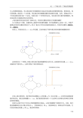

![4.2. ⼀个输⼊和⼀个输出的普遍性
x
−0.6
0.6
0.40
0.60
h = 0.6
1
−1
0
1
2
隐藏层的加权输出
试着将 h 值改⼤或改⼩,看看凸起的⾼度如何改变。试着把⾼度值改为负数,观察发⽣了什
么。并且试着改变阶跃点来看看如何改变凸起的形状。
顺便提⼀下,你会注意到,我们⽤神经元的⽅式,可以认为不只是在图形的⻆度,⽽且是更
传统的编程形式,作为 if-then-else 的⼀种声明,即:
if input >= step point:
add 1 to the weighted output
else:
add 0 to the weighted output
对于⼤部分内容,我将坚持以图形的考虑⻆度。但在接下来的内容中,你有时可能会发现交
换考虑⻆度是有帮助的,并且考虑 if-then-else 的形式。
我们可以⽤凸起制作的技巧来得到两个凸起,通过把两对隐藏神经元⼀起填充进同⼀个⽹
络:
x
h = −1.2
h = 0.3
0.40
0.60
0.70
0.90
1
−1
0
1
2
隐藏层的加权输出
这⾥我抑制了权重,只是简单地在每对隐藏神经元上写了 h 的值。试着增加和减少两个 h 值,
观察它如何改变图形。通过修改节点来移动凸起。
更普遍地,我们可以利⽤这个思想来取得我们想要的任何⾼度的峰值。尤其,我们可以把间
隔 [0, 1] 分成⼤量的⼦区间,⽤ N 表⽰,并利⽤ N 对隐藏神经元来设置任意期望⾼度的峰值。
让我们看看 N = 5 这如何⼯作。那样确实有很多神经元,所以我打算弄得挤⼀些。抱歉这个图
120](https://image.slidesharecdn.com/nndl-ebook5-160513104940/85/slide-130-320.jpg)


![4.2. ⼀个输⼊和⼀个输出的普遍性
x
0.6
0.4
0.4
0.2
0.6
0.8
0.2
0.0
0.8
1.0
0.2
0.8
h = −1.1
h = −1.4
h = −0.3
h = −1.0
h = 1.2
1
−2
−1
0
1
2
3
隐藏层的加权输出
你现在已经解决了所有⽹络的必要元素来近似计算函数 f(x)!这只是⼀个粗略的近似,但我
们可以很容易地做得更好,仅仅通过增加隐藏神经元对的数量,分配更多的凹凸形状。
特别是,将我们已经找到的所有数据转换回神经⽹络使⽤的标准参数设定是很容易的。让我
快速总结⼀下那是如何⼯作的。
第⼀层的权重都有⼀些⼤的,恒定的值,⽐如:w = 1000。
隐藏神经元上的偏置只是 b = −ws。例如,对于第⼆个隐藏神经元 s = 0.2 变成了 b =
−1000 × 0.2 = −200。
最后⼀层的权重由 h 值决定。例如,我们上⾯已经选择的第⼀个 h,h = −0.5,意味着顶部
两个隐藏神经元的相应的输出权重是 −0.5 和 0.5。如此等等,确定整个层的输出权重。
最后,输出神经元的偏置为 0。
这是所有要做的事情:现在我们有了⼀个可以很好计算我们原始⽬标函数的神经⽹络的完整
的描述。⽽且我们理解如何通过提⾼隐层神经元的数⽬来提⾼近似的质量。
更重要的是,关于我们的原始⽬标函数 f(x) = 0.2 + 0.4x2 + 0.3 sin(15x) + 0.05 cos(50x),没
有什么特别的。我们可以⽤这个程序计算任何定义域为 [0, 1],值域为 [0, 1] 的连续函数。在本质
上,我们使⽤我们的单层神经⽹络来建⽴⼀个函数的查找表。我们将能够建⽴这个思想,以提
供普遍性的⼀般性证明。
124](https://image.slidesharecdn.com/nndl-ebook5-160513104940/85/slide-134-320.jpg)


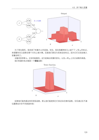


![5.1. 消失的梯度问题
5.1 消失的梯度问题
那么,在我们训练深度⽹络时究竟哪⾥出了问题?
为了回答这个问题,让我们重新看看使⽤单⼀隐藏层的神经⽹络⽰例。这⾥我们也是⽤
MNIST 数字分类问题作为研究和实验的对象3。
这⾥你也可以在⾃⼰的电脑上训练神经⽹络。或者就直接读下去。如果希望实际跟随这些步
骤,那就需要在电脑上安装 Python 2.7,Numpy 和代码,可以通过下⾯的命令复制所需要的代
码:
git clone https://github.com/mnielsen/neural-networks-and-deep-learning.git
如果你不使⽤ git,那么就直接从这⾥下载数据和代码。然后需要转⼊ src ⼦⽬录。
然后,在 Python 命令提⽰符中我们加载 MNIST 数据:
>>> import mnist_loader
>>> training_data, validation_data, test_data =
... mnist_loader.load_data_wrapper()
设置我们的⽹络:
>>> import network2
>>> net = network2.Network([784, 30, 10])
这个⽹络拥有 784 个输⼊层神经元,对应于输⼊图⽚的 28 × 28 = 784 个像素点。我们设置
隐藏层神经元为 30 个,输出层为 10 个神经元,对应于 10 个 MNIST 数字 (’0’, ’1’, ’2’, ..., 9)。
让我们训练 30 个完整的迭代期,使⽤⼩批量数据⼤⼩为 10,学习率 η = 0.1,规范化参数
λ = 5.0。在训练时,我们也会在 validation_data 上监控分类的准确度4:
>>> net.SGD(training_data, 30, 10, 0.1, lmbda=5.0,
... evaluation_data=validation_data, monitor_evaluation_accuracy=True)
最终我们得到了分类的准确率为 96.48%(也可能不同,每次运⾏实际上会有⼀点点的偏差)
这和我们前⾯的结果相似。
现在,我们增加另外⼀层隐藏层,同样地是 30 个神经元,试着使⽤相同的超参数进⾏训练:
>>> net = network2.Network([784, 30, 30, 10])
>>> net.SGD(training_data, 30, 10, 0.1, lmbda=5.0,
... evaluation_data=validation_data, monitor_evaluation_accuracy=True)
最终的结果分类准确度提升了⼀点,96.90%。这点令⼈兴奋:⼀点点的深度带来了效果。那
么就再增加⼀层同样的隐藏层:
>>> net = network2.Network([784, 30, 30, 30, 10])
>>> net.SGD(training_data, 30, 10, 0.1, lmbda=5.0,
... evaluation_data=validation_data, monitor_evaluation_accuracy=True)
哦,这⾥并没有什么提升,反⽽下降到了 96.57%,这与最初的浅层⽹络相差⽆⼏。再增加⼀
层:
>>> net = network2.Network([784, 30, 30, 30, 30, 10])
>>> net.SGD(training_data, 30, 10, 0.1, lmbda=5.0,
... evaluation_data=validation_data, monitor_evaluation_accuracy=True)
3
MNIST 问题和数据在这⾥和这⾥。
4
注意⽹络可能需要花费⼏分钟来训练,要看你机器的速度。所以如果你正在运⾏代码,你可能愿意继续阅读并稍
后回来,⽽不是等待代码完成执⾏。
142](https://image.slidesharecdn.com/nndl-ebook5-160513104940/85/slide-152-320.jpg)
![5.1. 消失的梯度问题
分类准确度⼜下降了,96.53%。这可能不是⼀个统计显著地下降,但是会让⼈们觉得沮丧。
这⾥表现出来的现象看起⾮常奇怪。直觉地,额外的隐藏层应当让⽹络能够学到更加复杂的
分类函数,然后可以在分类时表现得更好吧。可以肯定的是,事情并没有变差,⾄少新的层次
增加上,在最坏的情形下也就是没有影响5。事情并不是这样⼦的。
那么,应该是怎样的呢?假设额外的隐藏层的确能够在原理上起到作⽤,问题是我们的学习
算法没有发现正确地权值和偏置。那么现在就要好好看看学习算法本⾝有哪⾥出了问题,并搞
清楚如何改进了。
为了获得⼀些关于这个问题直觉上的洞察,我们可以将⽹络学到的东西进⾏可视化。下⾯,
我画出了⼀部分 [784, 30, 30, 10] 的⽹络,也就是包含两层各有 30 个隐藏神经元的隐藏层。图中
的每个神经元有⼀个条形统计图,表⽰这个神经元在⽹络进⾏学习时改变的速度。更⼤的条意
味着更快的速度,⽽⼩的条则表⽰变化缓慢。更加准确地说,这些条表⽰了每个神经元上的 ∂C
∂b ,
也就是代价函数关于神经元的偏置更变的速率。回顾第⼆章,我们看到了这个梯度的数值不仅
仅是在学习过程中偏置改变的速度,⽽且也控制了输⼊到神经元权重的变量速度。如果没有回
想起这些细节也不要担⼼:⽬前要记住的就是这些条表⽰了每个神经元权重和偏置在神经⽹络
学习时的变化速率。
为了让图⾥简单,我只展⽰出来最上⽅隐藏层上的 6 个神经元。这⾥忽略了输⼊层神经元,
因为他们并不包含需要学习的权重或者偏置。同样输出层神经元也忽略了,因为这⾥我们做的
是层层之间的⽐较,所以⽐较相同数量的两层更加合理啦。在⽹络初始化后⽴即得到训练前期
的结果如下6:
5
参⻅这个后⾯的问题来了解如何构建⼀个什么也不⼲的隐藏层。
6
绘制的数据图形由程序 generate_gradient.py ⽣成。同样的程序也⽤来⽣成本节后⾯引⽤的结果。
143](https://image.slidesharecdn.com/nndl-ebook5-160513104940/85/slide-153-320.jpg)
![5.1. 消失的梯度问题
hidden layer 1 hidden layer 2
该⽹络是随机初始化的,因此看到了神经元学习的速度差异其实很⼤。⽽且,我们可以发现,
第⼆个隐藏层上的条基本上都要⽐第⼀个隐藏层上的条要⼤。所以,在第⼆个隐藏层的神经元
将学习得更加快速。这仅仅是⼀个巧合么,或者第⼆个隐藏层的神经元⼀般情况下都要⽐第⼀
个隐藏层的神经元学习得更快?为了确定我们的猜测,拥有⼀种全局的⽅式来⽐较学习速度会
⽐较有效。我们这⾥将梯度表⽰为 δl
j = ∂C/∂bl
j 在第 l 层的第 j 个神经元的梯度。我们可以将 δ1
看做是⼀个向量其中元素表⽰第⼀层隐藏层的学习速度,δ2 则是第⼆层隐藏层的学习速度。接
着使⽤这些向量的⻓度作为全局衡量这些隐藏层的学习速度的度量。因此,||δ1|| 就代表第⼀层
隐藏层学习速度,⽽ ||δ2|| 就代表第⼆层隐藏层学习速度。借助这些定义,在和上图同样的配置
下,||δ1|| = 0.07 ⽽ ||δ2|| = 0.31,所以这就确认了之前的疑惑:在第⼆层隐藏层的神经元学习速
度确实⽐第⼀层要快。
如果我们添加更多的隐藏层呢?如果我们有三个隐藏层,⽐如说在⼀个 [784, 30, 30, 10] 的⽹
络中,那么对应的学习速度就是 0.012, 0.060, 0.283。这⾥前⾯的隐藏层学习速度还是要低于最
后的隐藏层。假设我们增加另⼀个包含 30 个隐藏神经元的隐藏层。那么,对应的学习速度就是:
0.003, 0.017, 0.070, 0.285。还是⼀样的模式:前⾯的层学习速度低于后⾯的层。
现在我们已经看到了训练开始时的学习速度,这是刚刚初始化之后的情况。那么这个速度会
随着训练的推移发⽣什么样的变化呢?让我们看看只有两个隐藏层。学习速度变化如下:
144](https://image.slidesharecdn.com/nndl-ebook5-160513104940/85/slide-154-320.jpg)
![5.1. 消失的梯度问题
0 100 200 300 400 500
Number of epochs of training
10-4
10-3
10-2
10-1
100 Speed of learning: 2 hidden layers
Hidden layer 1
Hidden layer 2
为了产⽣这些结果,我在 1000 个训练图像上进⾏了 500 轮 batch 梯度下降。这和我们通常
训练⽅式还是不同的 —— 我没有使⽤ minibatch,仅仅使⽤了 1000 个训练图像,⽽不是全部的
50, 000 幅图。我并不是想做点新鲜的尝试,或者蒙蔽你们的双眼,但因为使⽤ minibatch 随机
梯度下降会在结果中带来更多的噪声(尽管在平均噪声的时候结果很相似)。使⽤我已经确定的
参数可以对结果进⾏平滑,这样我们可以看清楚真正的情况是怎样的。如图所⽰,两层在开始
时就有着不同的速度。然后两层的学习速度在触底前迅速下落。在最后,我们发现第⼀层的学
习速度变得⽐第⼆层更慢了。
那么更加复杂的⽹络是什么情况呢?这⾥是⼀个类似的实验,但是这次有三个隐藏层
([784, 30, 30, 30, 10]):
0 100 200 300 400 500
Number of epochs of training
10-5
10-4
10-3
10-2
10-1
100 Speed of learning: 3 hidden layers
Hidden layer 1
Hidden layer 2
Hidden layer 3
同样,前⾯的隐藏层要⽐后⾯的隐藏层学习的更慢。最后⼀个实验,就是增加第四个隐藏层
([784, 30, 30, 30, 30, 10]),看看这⾥会发⽣什么:
145](https://image.slidesharecdn.com/nndl-ebook5-160513104940/85/slide-155-320.jpg)


![5.3. 在更加复杂⽹络中的不稳定梯度
到 σ′ 的两翼,这⾥会去到很⼩的值。唯⼀避免发⽣这个情况的⽅式是,如果输⼊激活函数掉⼊
相当狭窄的范围内(这个量化的解释在下⾯第⼀个问题中进⾏)。有时候,有可能会出现。但是
⼀般不⼤会发⽣。所以⼀般情况下,会遇到消失的梯度。
问题
• 考虑乘积 |wσ′(wa + b)|。假设有 |wσ′(wa + b)| >= 1。(1)这种情况只有在 |w| >= 4 的时
候才会出现。(2)假设 |w| >= 4,考虑那些满⾜ |wσ′(wa + b)| >= 1 的输⼊激活 a 集合。
证明:满⾜上述条件的该集合能够充满⼀个不超过 2
|w| ln(
|w|(1+
√
1−4/|w|)
2 − 1) 宽度的区间。
(3)数值上说明上述表达式在 |w| = 6.9 时候去的最⾼值约 0.45。所以即使每个条件都满
⾜,我们仍然有⼀个狭窄的输⼊激活区间,这样来避免消失的梯度问题。
• ⺓神经元:考虑⼀个单⼀输⼊的神经元,x,对应的权重 w1,偏差 b,输出上的权重 w2。
证明,通过合理选择权重和偏差,我们可以确保 w2σ(w1 ∗ x + b) = x 其中 x ∈ [0, 1]。这样
的神经元可⽤来作为⺓元使⽤,输出和输⼊相同(成⽐例)。提⽰:可以重写 x = 1/2 + ∆,
可以假设 w1 很⼩,和在 w1 ∗ ∆ 使⽤泰勒级数展开。
5.3 在更加复杂⽹络中的不稳定梯度
现在已经研究了简单的⽹络,每⼀层只包含⼀个神经元。那么那些每层包含很多神经元的更
加复杂的深度⽹络呢?
input layer
hidden layer 1 hidden layer 2 hidden layer 3
output layer
实际上,在这样的神经⽹络中,同样的情况也会发⽣。在前⾯关于反向传播的章节中,我们
看到了在⼀个共 L 层的第 l 层的梯度:
δl
= Σ′
(zl
)(wl+1
)T
Σ′
(zl+1
)(wl+2
)T
. . . Σ′
(zL
)∇aC (124)
这⾥ Σ′(zl) 是⼀个对⻆矩阵,每个元素是对第 l 层的带权输⼊ σ′(z)。⽽ wl 是对不同层的权
值矩阵。∇aC 是对每个输出激活的偏导数向量。
150](https://image.slidesharecdn.com/nndl-ebook5-160513104940/85/slide-160-320.jpg)


![6.1. 介绍卷积⽹络
input layer
hidden layer 1 hidden layer 2 hidden layer 3
output layer
特别地,对输⼊图像中的每个像素点,我们将其光强度作为对应输⼊层神经元的值。对于
28 × 28 像素的图像,这意味着我们的⽹络有 784(= 28 × 28)个输⼊神经元。我们然后训练⽹
络的权重和偏置,使得⽹络输出能够 —— 如我们希望地 —— 正确地辨认输⼊图像:’0’, ’1’, ’2’, ...,
’8’, or ’9’。
我们之前的⽹络⼯作得相当好:我们已经得到了超过 98% 的分类准确率,使⽤来⾃ MNIST
⼿写数字数据集的训练和测试数据。但是仔细推敲,使⽤全连接层的⽹络来分类图像是很奇怪
的。原因是这样的⼀个⽹络架构不考虑图像的空间结构。例如,它在完全相同的基础上去对待相
距很远和彼此接近的输⼊像素。这样的空间结构的概念必须从训练数据中推断。但是如果我们
使⽤⼀个设法利⽤空间结构的架构,⽽不是从⼀个⽩板状态的⽹络架构开始,会怎样?在这⼀
节中,我会描述卷积神经⽹络1。这些⽹络使⽤⼀个特别适⽤于分类图像的特殊架构。使⽤这个
架构使得卷积⽹络能跟快训练。相应的,这帮助我们训练深度的、多层的⽹络,它⾮常擅⻓于分
类图像。今天,深度卷积⽹络或者⼀些近似的变化形式,被⽤在⼤多数图像识别的神经⽹络中。
卷积神经⽹络采⽤了三种基本概念:局部感受野(local receptive fields),共享权重(shared
weights),和混合(pooling)。让我们逐个看下:
局部感受野: 在之前看到的全连接层的⽹络中,输⼊被描绘成纵向排列的神经元。但在⼀个
卷积⽹络中,把输⼊看作是⼀个 28 × 28 的⽅形排列的神经元更有帮助,其值对应于我们⽤作输
⼊的 28 × 28 的像素光强度:
1
最初的卷积神经⽹络要追溯到 1970 年代。但是建⽴起现代卷积⽹络学科的开创性论⽂是⼀篇 1998 年的
“Gradient-based learning applied to document recognition”,作者为 Yann LeCun,Léon Bottou,Yoshua Bengio,和
Patrick Haffner。LeCun ⾃那以后做了⼀个关于卷积⽹络术语的有趣评论:“以类似卷积⽹络模型的[⽣物学上的]神
经系统原型是⾮常牵强的。这正是为什么我把它们称为‘卷积⽹络’⽽不是‘卷积神经⽹络’,以及为什么我们称这
些节点为‘单元’⽽不是‘神经元’”。尽管有这样的评论,卷积⽹络使⽤许多我们⽬前为⽌学习到的神经⽹络相同的
思想:诸如反向传播,梯度下降,规范化,⾮线性激活函数等等。所以我们会遵循常规惯例,认为它们是神经⽹络的
⼀种类型。我会交换地使⽤术语“卷积神经⽹络”和“卷积⽹络(⾏为)”。我也会交换地使⽤术语“[⼈⼯]神经元”
和“单元”。
154](https://image.slidesharecdn.com/nndl-ebook5-160513104940/85/slide-164-320.jpg)


![6.2. 卷积神经⽹络在实际中的应⽤
network3.py,它是前⾯章节开发的 network.py 和 network2.py 的强化版本7。如果你想跟着学,代
码可以从 GitHub 上下载。注意我们将在下⼀节中解决 network3.py 需要的代码。在这⼀节中,我
们将把 network3.py 作为库来构建卷积⽹络。
程序 network.py 和 network2.py 是⽤ Python 和矩阵库 Numpy 实现的。这些程序从最初的原
理⼯作,并致⼒于反向传播、随即梯度下降等细节。但是现在我们已经理解了这些细节,对于
network3.py 我们打算使⽤⼀个称为 Theano 的机器学习库8。使⽤ Theano 使得实现针对卷积神
经⽹络的反向传播很容易,因为它⾃动计算涉及到的映射。Theano 也⽐我们前⾯代码更快(那
些代码是为了容易理解,不是为了运⾏速度),这使它可实际⽤于训练更复杂的⽹络。特别地,
Theano 的⼀个⾮常好的特性是它能够运⾏于 CPU 或者,如果可以,GPU 上。运⾏于 GPU 上可
以提供显著的增速,⽽且,有助于实际⽤于更复杂的⽹络。
如果你想要跟着学,你需要可运⾏在你的系统上的 Theano。按照项⽬主⻚上的说明来安装
Theano。接下来的例⼦使⽤ Theano 0.69 运⾏过。有些在没有 GPU ⽀持的 Mac OS X Yosemite
运⾏过。有些在有 NVIDIA GPU ⽀持的 Ubuntu 14.04 中运⾏过。有些实验在两个系统中都运⾏
过。为了让 networks3.py 运⾏,你需要(适当地)把 networks3.py 源码中的 GPU 标志设置为 True 或
者 False。此外,为了让 Theano 运⾏于 GPU 上,你可能会发现这份指导说明有帮助。互联⽹上
也有教程,很容易⽤ Google 搜索到,同样能帮助你让 Theano ⼯作。如果你⼿上的系统没有可
⽤的 GPU,那么你可能想要看下 Amazon Web Services EC2 G2 实例类型。注意即使有 GPU ⽀
持,代码仍然需要⼀些时间执⾏。许多实验要花费从⼏分钟到⼏个⼩时的时间来运⾏。在 CPU
上可能需要花费数天时间来运⾏最复杂的实验。正如前⾯章节⾥说的,我建议让程序运⾏着,同
时继续阅读,偶尔回来检查下代码的输出。如果你⽤的是 CPU,你可能需要对更复杂的实验减
少训练迭代期的数量,或者整个忽略它们。
为了取得⼀个基线,我们将从⼀个浅层架构开始,它仅仅使⽤⼀个隐藏层,包含 100 个隐藏
神经元。我们会训练 60 迭代期,使⽤学习速率为:η = 0.1,⼩批量数据 ⼤⼩为 10,没有规范
化。这样运⾏10:
>>> import network3
>>> from network3 import Network
>>> from network3 import ConvPoolLayer, FullyConnectedLayer, SoftmaxLayer
>>> training_data, validation_data, test_data = network3.load_data_shared()
>>> mini_batch_size = 10
>>> net = Network([
FullyConnectedLayer(n_in=784, n_out=100),
SoftmaxLayer(n_in=100, n_out=10)], mini_batch_size)
>>> net.SGD(training_data, 60, mini_batch_size, 0.1,
validation_data, test_data)
我获得的⼀个最好的分类准确率是 97.80%。这是 test_data 上的分类准确率,在这个取值的
训练迭代期的地⽅,我们在validation_data上得到了最好的分类准确率。使⽤验证数据来决定在
何时对测试准确率估值有助于避免测试数据上的过度拟合(⻅前⾯关于验证数据使⽤的讨论)。
我们将在下⾯遵循这个习惯。你的结构可能稍有不同,因为⽹络的权重和偏置是随机初始化
7
注意 network3.py 包含了源⾃ Theano 库⽂档中关于卷积神经⽹络(尤其是 LeNet-5 的实现),Misha Denil 的弃
权的实现,以及 Chris Olah 的概念。
8
参⻅ Theano: A CPU and GPU Math Expression Compiler in Python,作者为 James Bergstra,Olivier Breuleux,
Frederic Bastien,Pascal Lamblin,Ravzan Pascanu,Guillaume Desjardins,Joseph Turian,David Warde-Farley,和
Yoshua Bengio (2010)。Theano 也是流⾏的 Pylearn2 和 Keras 神经⽹络库的基础。其它在本⽂写作时流⾏的神经
⽹路库包括 Caffe 和 Torch。
9
当我发布这⼀章时,Theano 的当前版本变成了 0.7。我实际上已经在 Theano 0.7 版本中重新运⾏过这些例⼦并
取得了和⽂中⾮常相似的结果。
10
本节中的实验代码可以在 这个脚本中找到。注意,脚本中的代码只是简单地重复并相对于本节中的讨论。
161](https://image.slidesharecdn.com/nndl-ebook5-160513104940/85/slide-171-320.jpg)
![6.2. 卷积神经⽹络在实际中的应⽤
的11。
这个 97.80% 的准确率接近于第三章中获得的 98.04% 的准确率,使⽤⼀个相似的⽹络架构和
学习超参数。特别地,两个例⼦都使⽤⼀个浅层⽹络,具有单个包含有 100 个隐藏神经元的隐
藏层。两者都训练 60 个 迭代期,⼩批量数据⼤⼩为 10,学习速率 为 η = 0.1。
然⽽,在之前的⽹络中有两个不同的地⽅。⾸先,我们规范化了之前的⽹络,来帮助降低过
度拟合带来的影响。规范化当前的⽹络确实可以提⾼准确率,但是得到的只是很⼩,所以我们
将推迟到后⾯再来惦记规范化。第⼆,虽然之前的⽹络中的最终层使⽤了 S 型激活值和交叉熵
代价函数,当前⽹络使⽤⼀个柔性最⼤值的最终层,以及对数似然代价函数。正如第三章中解
释的,这不是⼀个⼤的改变。我没有为了任何特别深刻的原因来做出这样的改变 —— 主要是因
为柔性最⼤值和对数似然代价在现代的图像分类⽹络中很常⻅。
我们能⽤⼀个更深的⽹络架构来做得⽐这些结果更好吗?
让我们从在⽹络开始位置的右边插⼊⼀个卷积层开始。我们将使⽤ 5 × 5 局部感受野,跨距
为 1,20 个特征映射。我们也会插⼊⼀个最⼤值混合层,它⽤⼀个 2 × 2 的混合窗⼝来合并特征。
所以总体的⽹络架构看起来很像上⼀节讨论的架构,但是有⼀个额外的全连接层:
28 × 28
convolution layer
20 × 24 × 24 pooling layer
20 × 12 × 12
100 sigmoid
neurons
10 neurons
output layer
(softmax)
...
...
在这个架构中,我们可以把卷积和混合层看作是在学习输⼊训练图像中的局部感受野,⽽后
⾯的全连接层则在⼀个更抽象的层次学习,从整个图像整合全局信息。这是⼀种常⻅的卷积神
经⽹络模式。
让我们训练这样的⼀个⽹络,看看它表现怎样12:
>>> net = Network([
ConvPoolLayer(image_shape=(mini_batch_size, 1, 28, 28),
filter_shape=(20, 1, 5, 5),
poolsize=(2, 2)),
FullyConnectedLayer(n_in=20*12*12, n_out=100),
SoftmaxLayer(n_in=100, n_out=10)], mini_batch_size)
>>> net.SGD(training_data, 60, mini_batch_size, 0.1,
validation_data, test_data)
11
实际上,在这个实验中我其实对这个架构的⽹络运⾏了三次独⽴的训练。然后我从这三次运⾏中报告了对应于最
佳验证准确率的测试准确率。利⽤多次运⾏有助于减少结果中的变动,它在⽐较许多个架构时是很有⽤的,正如我
们正在做的。除⾮明确指出,我在下⾯已经遵循了这个程序。在实践中,它对于所获得的结果不会带来什么区别。
12
这⾥我继续使⽤⼀个⼤⼩为 10 的⼩批量数据。正如我们前⾯讨论过的,使⽤更⼤的⼩批量数据可能提⾼训练速
度。我继续使⽤相同的⼩批量数据,主要是为了和前⾯章节中的实验保持⼀致。
162](https://image.slidesharecdn.com/nndl-ebook5-160513104940/85/slide-172-320.jpg)
![6.2. 卷积神经⽹络在实际中的应⽤
我们得到了 98.78% 的准确率,这是相当⼤的改善,超过了我们以前结构的任何⼀个。事实
上,我们已经减少了超过三分之⼀的错误率,这是⼀个很⼤的进步。
在指定⽹络结构时,我把卷积和混合层作为⼀个单⼀层对待。不管他们是被视为分开的层还
是作为⼀个单⼀的层在⼀定程度上是⼀个个⼈喜好的问题。network3.py 视他们为单个层,因为
它使得 network3.py 的代码更紧凑。然⽽,如果需要的话,很容易修改 network3.py 使得这些层可
以单独指定。
练习
• 如果你删除了全连接层,只使⽤卷积–混合层和柔性最⼤值层,你得到了什么样的分类准
确率?全连接层的加⼊有帮助吗?
我们能改进 98.78% 的分类准确率吗?
让我们试着插⼊第⼆个卷积–混合层。把它插在已有的卷积–混合层和全连接隐藏层之间。我
们再次使⽤⼀个 5 × 5 局部感受野,混合 2 × 2 的区域。让我们看看⽤前⾯相似的超参数训练会
发⽣什么:
>>> net = Network([
ConvPoolLayer(image_shape=(mini_batch_size, 1, 28, 28),
filter_shape=(20, 1, 5, 5),
poolsize=(2, 2)),
ConvPoolLayer(image_shape=(mini_batch_size, 20, 12, 12),
filter_shape=(40, 20, 5, 5),
poolsize=(2, 2)),
FullyConnectedLayer(n_in=40*4*4, n_out=100),
SoftmaxLayer(n_in=100, n_out=10)], mini_batch_size)
>>> net.SGD(training_data, 60, mini_batch_size, 0.1,
validation_data, test_data)
再⼀次,我们得到了改善:现在我们达到了 99.06% 的分类准确率。
在这⾥有两个很⾃然想到的问题。第⼀个问题是:应⽤第⼆个卷积–混合层意味着什么?实
际上,你可以认为第⼆个卷积–混合层输⼊ 12 × 12 幅“图像”,其“像素”代表原始输⼊图像中
特定的局部特征的存在(或不存在)。所以你可以认为这⼀层输⼊原始输⼊图像的⼀个版本。这
个版本是经过抽象和凝缩过的,但是仍然有⼤量的空间结构,所以使⽤第⼆个卷积–混合层是有
意义的。
这是⼀个令然满意的观点,但是引出了第⼆个问题。从前⾯层的输出涉及 20 个独⽴的特征
映射,所以对第⼆个卷积–混合层有 20 × 20 × 12 个输⼊。就好像我们有 20 幅单独的图像输⼊
给卷积–混合层,⽽不是第⼀个卷积–混合层情况下的单幅图像。第⼆个卷积–混合层⾥的神经
元应该如何响应这些多重的输⼊图像呢?实际上,我们将允许这⼀层中的每个神经元从它的局
部感受野中的所有 20 × 5 × 5 输⼊神经元学习。更⾮正式的:第⼆个卷积–混合层中的特征检测
器可访问所有前⾯层的特征,但仅在其特定的局部感受野中13。
问题
• 使⽤ tanh 激活函数 在本书前⾯我已经⼏次提起过tanh 函数可以是⼀个⽐ S 型函数更好
的激活函数。我们还没有实际采⽤过这些建议,因为我们已经⽤ S 型取得了⼤量进展。但
13
如果输⼊图像是有颜⾊的,这个问题会在第⼀层中出现。在这种情况下,对于每⼀个像素我们会有 3 个输⼊特
征,对应于输⼊图像中的红⾊、绿⾊和蓝⾊通道。因此我们将允许特征检测器可访问所有颜⾊信息,但仅仅在⼀个
给定的局部感受野中。
163](https://image.slidesharecdn.com/nndl-ebook5-160513104940/85/slide-173-320.jpg)
![6.2. 卷积神经⽹络在实际中的应⽤
现在让我们试试⼀些⽤ tanh 作为我们激活函数的实验。试着训练卷积和全连接层中具有
tanh 激活值的⽹络14。开始时使⽤ S 型⽹络中使⽤的相同的超参数,但是训练 20 个迭代
期,⽽不是 60 个。你的⽹络表现得怎么样?如果你继续训练到 60 个迭代期会怎样?试着
将 tanh 和 S 型⽹络的每个迭代期的验证准确率都绘制出来,都绘制到 60 个迭代期。如果
你的结果和我的相似,你会发现 tanh ⽹络训练得稍微快些,但是最终的准确率⾮常相似。
你能否解释为什么 tanh ⽹络可以训练得更快?你能否⽤ S 型取得⼀个相似的训练速度,也
许通过改变学习速率,或者做些调整15?试着⽤五六个迭代学习超参数和⽹络架构,寻找
tanh 优于 S 型的⽅⾯。注意:这是⼀个开放式问题。就我个⼈⽽⾔,我并没有找到太多切
换为 tanh 的优势,虽然我没全⾯地做过实验,也许你会找到⼀个⽅法。⽆论如何,我们
⻢上会发现切换到修正线性激活函数的⼀个优势,所以我们不会去深⼊使⽤ tanh 函数。。
使⽤修正线性单元: 到现在为⽌,我们开发的⽹络实际上是⼀篇开创性的 1998 论⽂16 中使
⽤的众多⽹络中⼀种的变化形式,这个⽹络被称为 LeNet-5,并引⼊了 MNIST 问题。这为进⼀
步实验并构筑理解和直观感受打下很好的基础。特别是,有很多种我们可以改变⽹络来改善结
果的⽅式。
作为开始,让我们改变我们的神经元,我们使⽤修正线性单元⽽不是 S 型激活函数。确切地
说,我们将使⽤激活函数 f(z) ≡ max(0, z)。我们将训练 60 个 迭代期,学习速率为 η = 0.03。我
也发现⽤⼀些 L2 规范化也有点帮助,使⽤规范化参数 λ = 0.1:
>>> from network3 import ReLU
>>> net = Network([
ConvPoolLayer(image_shape=(mini_batch_size, 1, 28, 28),
filter_shape=(20, 1, 5, 5),
poolsize=(2, 2),
activation_fn=ReLU),
ConvPoolLayer(image_shape=(mini_batch_size, 20, 12, 12),
filter_shape=(40, 20, 5, 5),
poolsize=(2, 2),
activation_fn=ReLU),
FullyConnectedLayer(n_in=40*4*4, n_out=100, activation_fn=ReLU),
SoftmaxLayer(n_in=100, n_out=10)], mini_batch_size)
>>> net.SGD(training_data, 60, mini_batch_size, 0.03,
validation_data, test_data, lmbda=0.1)
我得到⼀个 99.23% 的分类准确率。它稍微超过了 S 型的结果(99.06)。然⽽,在我所有实
验中我发现基于修正线性单元的⽹络,其性能始终优于基于 S 型激活函数的⽹络。似乎对于这
个问题切换到修正线性单元确实有收益。
是什么使得修正线性激活函数好于 S 型或者 tanh 函数?⽬前,我们对这个问题的答案有⼀
个很差的理解。实际上,修正线性单元只在过去⼏年才开始被⼴泛使⽤。最近才采⽤的原因是
以经验为依据的:⼀些⼈经常基于直觉或者启发式的理由试着⽤修正线性单元17。他们在分类
基准数据集时取得了很好的结果,并且其实践传播开了。在⼀个理想的世界中,我们有⼀个理
论告诉我们为什么样的应⽤选择什么样的激活函数。但⽬前我们我们离这样的理想世界还有⼀
条很⻓的路。如果通过选择⼀个更好的激活函数来取得了进⼀步的重⼤改进,我⼀点也不会感
14
注意你可以将 activation_fn=tanh 作为⼀个参数传递给 ConvPoolLayer 和 FullyConnectedLayer 类。
15
你也许可以回想 σ(z) = (1 + tanh(z/2))/2 来找灵感。
16
”Gradient-based learning applied to document recognition”,作者为 Yann LeCun,Léon Bottou,Yoshua Bengio,
和 Patrick Haffner (1998)。细节上有很多不同,但⼤体上讲,我们的⽹络和论⽂中描述的⽹络⾮常相似。
17
⼀个通常的理由是 max(0, z) 在 z 取最⼤极限时不会饱和,不像 S 型神经元,⽽这有助于修正线性单元持续学习。
到⽬前为⽌,这⼀辩解很好,但不是⼀个详细的理由,更多的是⼀个“就这样”的故事。注意我们在第⼆章⾥讨论过
饱和的问题。
164](https://image.slidesharecdn.com/nndl-ebook5-160513104940/85/slide-174-320.jpg)
![6.2. 卷积神经⽹络在实际中的应⽤
到惊讶,我还期待在未来的⼏⼗年⾥,⼀个强⼤的激活函数理论将被开发。今天,我们仍然不
得不依靠单凭经验的不⾜的理解。
扩展训练数据: 另⼀种我们可能希望改进结果的⽅法是以算法形式扩展训练数据。扩展训
练数据的⼀个简单的⽅法是将每个训练图像由⼀个像素来代替,⽆论是上⼀个像素,⼀个像素,
左边⼀个像素,或右边⼀个像素。我们可以通过在 shell 提⽰符中运⾏程序 expand_mnist.py 来这
样做18:
$ python expand_mnist.py
运⾏这个程序取得 50, 000 幅 MNIST 训练图像并扩展为具有 250, 000 幅训练图像的训练集。
然后我们可以使⽤这些训练图像来训练我们的⽹络。我们将使⽤和上⾯⼀样的具有修正线性单
元的⽹络。在我初始的实验中我减少了训练迭代期的数量 —— 这讲得通,因为我们在训练 5 倍
的数据。但是实际上,扩展数据结果是相当多地减少了过度拟合的影响。所有,在做了⼀些实
验后,我最终回到训练 60 个迭代期。不管怎样,让我们训练:
>>> expanded_training_data, _, _ = network3.load_data_shared(
"../data/mnist_expanded.pkl.gz")
>>> net = Network([
ConvPoolLayer(image_shape=(mini_batch_size, 1, 28, 28),
filter_shape=(20, 1, 5, 5),
poolsize=(2, 2),
activation_fn=ReLU),
ConvPoolLayer(image_shape=(mini_batch_size, 20, 12, 12),
filter_shape=(40, 20, 5, 5),
poolsize=(2, 2),
activation_fn=ReLU),
FullyConnectedLayer(n_in=40*4*4, n_out=100, activation_fn=ReLU),
SoftmaxLayer(n_in=100, n_out=10)], mini_batch_size)
>>> net.SGD(expanded_training_data, 60, mini_batch_size, 0.03,
validation_data, test_data, lmbda=0.1)
使⽤扩展后的训练数据我取得了⼀个 99.37% 的训练准确率。所以这个⼏乎是微不⾜道的改
变在分类准确率上给出了⼀个显著的改进。事实上,正如我们前⾯所讨论的,这种以算法形式
扩展数据的想法可以更进⼀步。提醒你⼀些早期讨论的结果:在 2003 年,Simard,Steinkraus
和 Platt19 使⽤⼀个神经⽹络改进了他们的 MNIST 性能,达到了 99.6%,这个⽹络以其它⽅式和
我们的⾮常相似,使⽤两个卷积–混合层,跟着⼀个具有 100 个神经元的隐藏的全连接层。在他
们的架构中有⼀些细节上的不同 —— 例如他们没有利⽤修正线性单元 —— 但是他们改进性能的
关键是扩展训练数据。他们通过旋转,位移和扭曲 MNIST 训练图像来扩展。他们还开发了⼀个
“弹性扭曲”的流程,⼀种模拟当⼀个⼈写字时⼿部肌⾁随机振动的⽅式。通过组合所有这些流
程,他们相当⼤地增加了训练数据的有效规模,⽽这就是他们如何达到 99.6% 准确率的。
问题
• 卷积层的想法是以⼀种横跨图像不变的⽅式作出反应。它看上去令⼈惊奇,然⽽,当我们
做完所有输⼊数据的转换,⽹络能学习得更多。你能否解释为什么这实际上很合理?
插⼊⼀个额外的全连接层: 我们还能做得更好吗?⼀种可能性是使⽤和上⾯完全相同的程
18
expand_mnist.py 的代码可以从这⾥获取。
19
Best Practices for Convolutional Neural Networks Applied to Visual Document Analysis,作者为 Patrice Simard,
Dave Steinkraus,和 John Platt (2003)。
165](https://image.slidesharecdn.com/nndl-ebook5-160513104940/85/slide-175-320.jpg)
![6.2. 卷积神经⽹络在实际中的应⽤
序,但是扩展全连接层的规模。我试过 300 和 1, 000 个神经元,分别取得了 99.46% 和 99.43%。
这很有趣,但对于前⾯的结果(99.37%)并不是⼀个令⼈信服的超越。
增加⼀个额外的全连接层怎样?让我们试着插⼊⼀个全连接层,这样我们就有两个 100 个隐
藏神经元的全连接层:
>>> net = Network([
ConvPoolLayer(image_shape=(mini_batch_size, 1, 28, 28),
filter_shape=(20, 1, 5, 5),
poolsize=(2, 2),
activation_fn=ReLU),
ConvPoolLayer(image_shape=(mini_batch_size, 20, 12, 12),
filter_shape=(40, 20, 5, 5),
poolsize=(2, 2),
activation_fn=ReLU),
FullyConnectedLayer(n_in=40*4*4, n_out=100, activation_fn=ReLU),
FullyConnectedLayer(n_in=100, n_out=100, activation_fn=ReLU),
SoftmaxLayer(n_in=100, n_out=10)], mini_batch_size)
>>> net.SGD(expanded_training_data, 60, mini_batch_size, 0.03,
validation_data, test_data, lmbda=0.1)
这样做我取得⼀个 99.43% 的测试准确率。再⼀次,扩展后的⽹络并没有帮助太多。运⾏类
似的试验,⽤包含 300 和 1, 000 个隐藏神经元的全连接层产⽣ 99.48% 和 99.47% 的结果。这是令
⼈⿎舞的,但仍然缺乏⼀个真正决定性的胜利。
这⾥发⽣了什么事?扩展的,或者额外的全连接层真的对 MNIST 没帮助吗?或者说,我们
的⽹络有能⼒做得更好,但我们在⽤错误的⽅式学习?例如,也许我们可以⽤更强有⼒的规范
化技术来减⼩过度拟合的趋势。⼀种可能性是第三章介绍的弃权技术。回想弃权的基本思想是
在训练⽹络时随机地移除单独的激活值。这使得模型对单独依据的丢失更为强劲,因此不太可
能依赖于训练数据的特质。让我们试着应⽤弃权到最终的全连接层:
>>> net = Network([
ConvPoolLayer(image_shape=(mini_batch_size, 1, 28, 28),
filter_shape=(20, 1, 5, 5),
poolsize=(2, 2),
activation_fn=ReLU),
ConvPoolLayer(image_shape=(mini_batch_size, 20, 12, 12),
filter_shape=(40, 20, 5, 5),
poolsize=(2, 2),
activation_fn=ReLU),
FullyConnectedLayer(
n_in=40*4*4, n_out=1000, activation_fn=ReLU, p_dropout=0.5),
FullyConnectedLayer(
n_in=1000, n_out=1000, activation_fn=ReLU, p_dropout=0.5),
SoftmaxLayer(n_in=1000, n_out=10, p_dropout=0.5)],
mini_batch_size)
>>> net.SGD(expanded_training_data, 40, mini_batch_size, 0.03,
validation_data, test_data)
使⽤它,我们取得了 99.60% 的准确率,这是⼀个显著的超越我们前⾯结果的进步,尤其是
我们主要的基准,具有 100 个隐藏神经元的⽹络,其中我们达到了 99.37%。
有两个值得注意的变化。
⾸先,我减少了训练迭代期的数量到 40:弃权减少了过度拟合,所以我们学习得更快。
其次,全连接隐藏层有 1, 000 个神经元,不是之前使⽤的 100 个。当然,在训练时弃权有效
地忽略了很多神经元。所以⼀些扩充是可以预期的。实际上,我试过⽤ 300 和 1, 000 个隐藏神经
元的实验,⽤ 1, 000 个隐藏神经元(⾮常略微地)取得了更好的验证性能。
166](https://image.slidesharecdn.com/nndl-ebook5-160513104940/85/slide-176-320.jpg)


![6.3. 卷积⽹络的代码
得深度学习的定义像是时刻就有结果的事。深度学习中实际的突破是认识到它超过浅的 1、2 层
的⽹络是切实可⾏的,这样的浅层⽹络直到 2000 年中都占据优势。这确实是⼀个重⼤的突破,
开启了更多有特殊意义的模型的探索。但除这之外,层的数⽬并不是主要的基本利益关系。更
确切地说,使⽤更深层的⽹络是⼀种⽤来帮助实现其他⽬标⼯具 —— 例如更好的分类精确率。
⼀些按部就班的话: 在这⼀节中,我们从单个隐藏层的浅层⽹络顺利转换到多层卷积⽹络。
这⼀切似乎很容易!我们做了⼀个改变,其中⼤部分,我们得到了改进。如果你开始尝试,我可
以保证事情不会总是那么顺利。原因是,我呈现的是⼀个清理过的叙述,省略了许多实验 ——
包括许多失败的实验。这个清理过的叙述,希望能帮助你清楚认识基本思想。但它也有⻛险,传
达着不完整的感觉。取得⼀个好的,可⼯作的⽹络会涉及到⼤量的试验和错误,偶尔有挫折。在
实践中,你应该预计会处理相当多的实验。为了加快这⼀进程,你可能会发现回顾第三章关于如
何选择⼀个神经⽹络的超参数的讨论会有帮助,或许也看⼀些那⼀⼩节中的进⼀步阅读的建议。
6.3 卷积⽹络的代码
好了,现在来看看我们的卷积⽹络代码,network3.py。整体看来,程序结构类似于 network2.py,
尽管细节有差异,因为我们使⽤了 Theano。⾸先我们来看 FullyConnectedLayer 类,这类似于我
们之前讨论的那些神经⽹络层。下⾯是代码
class FullyConnectedLayer(object):
def __init__(self, n_in, n_out, activation_fn=sigmoid, p_dropout=0.0):
self.n_in = n_in
self.n_out = n_out
self.activation_fn = activation_fn
self.p_dropout = p_dropout
# Initialize weights and biases
self.w = theano.shared(
np.asarray(
np.random.normal(
loc=0.0, scale=np.sqrt(1.0/n_out), size=(n_in, n_out)),
dtype=theano.config.floatX),
name='w', borrow=True)
self.b = theano.shared(
np.asarray(np.random.normal(loc=0.0, scale=1.0, size=(n_out,)),
dtype=theano.config.floatX),
name='b', borrow=True)
self.params = [self.w, self.b]
def set_inpt(self, inpt, inpt_dropout, mini_batch_size):
self.inpt = inpt.reshape((mini_batch_size, self.n_in))
self.output = self.activation_fn(
(1-self.p_dropout)*T.dot(self.inpt, self.w) + self.b)
self.y_out = T.argmax(self.output, axis=1)
self.inpt_dropout = dropout_layer(
inpt_dropout.reshape((mini_batch_size, self.n_in)), self.p_dropout)
self.output_dropout = self.activation_fn(
T.dot(self.inpt_dropout, self.w) + self.b)
def accuracy(self, y):
"Return the accuracy for the mini-batch."
return T.mean(T.eq(y, self.y_out))
__init__ ⽅法中的⼤部分都是可以⾃解释的,这⾥再给出⼀些解释。我们根据正态分布随
169](https://image.slidesharecdn.com/nndl-ebook5-160513104940/85/slide-179-320.jpg)
![6.3. 卷积⽹络的代码
机初始化了权重和偏差。代码中对应这个操作的⼀⾏看起来可能很吓⼈,但其实只在进⾏载⼊
权重和偏差到 Theano 中所谓的共享变量中。这样可以确保这些变量可在 GPU 中进⾏处理。对
此不做过深的解释。如果感兴趣,可以查看 Theano 的⽂档。⽽这种初始化的⽅式也是专⻔为
sigmoid 激活函数设计的(参⻅这⾥)。理想的情况是,我们初始化权重和偏差时会根据不同的
激活函数(如 tanh 和 Rectified Linear Function)进⾏调整。这个在下⾯的问题中会进⾏讨论。
初始⽅法 __init__ 以 self.params = [self.W, self.b] 结束。这样将该层所有需要学习的参数都归
在⼀起。后⾯,Network.SGD ⽅法会使⽤ params 属性来确定⽹络实例中什么变量可以学习。
set_inpt ⽅法⽤来设置该层的输⼊,并计算相应的输出。我使⽤ inpt ⽽⾮ input 因为在 python
中 input 是⼀个内置函数。如果将两者混淆,必然会导致不可预测的⾏为,对出现的问题也难以
定位。注意我们实际上⽤两种⽅式设置输⼊的:self.input 和 self.inpt_dropout。因为训练时我们
可能要使⽤ dropout。如果使⽤ dropout,就需要设置对应丢弃的概率 self.p_dropout。这就是在
set_inpt ⽅法的倒数第⼆⾏ dropout_layer 做的事。所以 self.inpt_dropout 和 self.output_dropout
在训练过程中使⽤,⽽ self.inpt 和 self.output ⽤作其他任务,⽐如衡量验证集和测试集模型的
准确度。
ConvPoolLayer 和 SoftmaxLayer 类定义和 FullyConnectedLayer 定义差不多。所以我这⼉不会给
出代码。如果你感兴趣,可以参考本节后⾯的 network3.py 的代码。
尽管这样,我们还是指出⼀些重要的微弱的细节差别。明显⼀点的是,在 ConvPoolLayer 和
SoftmaxLayer 中,我们采⽤了相应的合适的计算输出激活值⽅式。幸运的是,Theano 提供了内
置的操作让我们计算卷积、max-pooling 和 softmax 函数。
不⼤明显的,在我们引⼊ softmax layer 时,我们没有讨论如何初始化权重和偏差。其他地
⽅我们已经讨论过对 sigmoid 层,我们应当使⽤合适参数的正态分布来初始化权重。但是这个
启发式的论断是针对 sigmoid 神经元的(做⼀些调整可以⽤于 tanh 神经元上)。但是,并没有特
殊的原因说这个论断可以⽤在 softmax 层上。所以没有⼀个先验的理由应⽤这样的初始化。与
其使⽤之前的⽅法初始化,我这⾥会将所有权值和偏差设置为 0。这是⼀个 ad hoc 的过程,但
在实践使⽤过程中效果倒是很不错。
好了,我们已经看过了所有关于层的类。那么 Network 类是怎样的呢?让我们看看 __init__
⽅法:
class Network(object):
def __init__(self, layers, mini_batch_size):
"""Takes a list of `layers`, describing the network architecture, and
a value for the `mini_batch_size` to be used during training
by stochastic gradient descent.
"""
self.layers = layers
self.mini_batch_size = mini_batch_size
self.params = [param for layer in self.layers for param in layer.params]
self.x = T.matrix("x")
self.y = T.ivector("y")
init_layer = self.layers[0]
init_layer.set_inpt(self.x, self.x, self.mini_batch_size)
for j in xrange(1, len(self.layers)):
prev_layer, layer = self.layers[j-1], self.layers[j]
layer.set_inpt(
prev_layer.output, prev_layer.output_dropout, self.mini_batch_size)
self.output = self.layers[-1].output
self.output_dropout = self.layers[-1].output_dropout
170](https://image.slidesharecdn.com/nndl-ebook5-160513104940/85/slide-180-320.jpg)
![6.3. 卷积⽹络的代码
这段代码⼤部分是可以⾃解释的。self.params = [param for layer in ...] 此⾏代码对每层的
参数捆绑到⼀个列表中。Network.SGD ⽅法会使⽤ self.params 来确定 Network 中哪些变量需要学
习。⽽ self.x = T.matrix("x") 和 self.y = T.ivector("y") 则定义了 Theano 符号变量 x 和 y。这
些会⽤来表⽰输⼊和⽹络得到的输出。
这⾥不是 Theano 的教程,所以不会深度讨论这些变量指代什么东西。但是粗略的想法就是
这些代表了数学变量,⽽⾮显式的值。我们可以对这些变量做通常需要的操作:加减乘除,作
⽤函数等等。实际上,Theano 提供了很多对符号变量进⾏操作⽅法,如卷积、最⼤值混合等等。
但是最重要的是能够进⾏快速符号微分运算,使⽤反向传播算法⼀种通⽤的形式。这对于应⽤
随机梯度下降在若⼲种⽹络结构的变体上特别有效。特别低,接下来⼏⾏代码定义了⽹络的符
号输出。我们通过下⾯这⾏
init_layer.set_inpt(self.x, self.x, self.mini_batch_size)
设置初始层的输⼊。
请注意输⼊是以每次⼀个 mini-batch 的⽅式进⾏的,这就是⼩批量数据⼤⼩为何要指定的原
因。还需要注意的是,我们将输⼊ self.x 传了两次:这是因为我们我们可能会以两种⽅式(有
dropout 和⽆ dropout)使⽤⽹络。for 循环将符号变量 self.x 通过 Network 的层进⾏前向传播。
这样我们可以定义最终的输出 output 和 output_dropout 属性,这些都是 Network 符号式输出。
现在我们理解了 Network 是如何初始化了,让我们看看它如何使⽤ SGD ⽅法进⾏训练的。代
码看起来很⻓,但是它的结构实际上相当简单。代码后⾯也有⼀些注解。
def SGD(self, training_data, epochs, mini_batch_size, eta,
validation_data, test_data, lmbda=0.0):
"""Train the network using mini-batch stochastic gradient descent."""
training_x, training_y = training_data
validation_x, validation_y = validation_data
test_x, test_y = test_data
# compute number of minibatches for training, validation and testing
num_training_batches = size(training_data)/mini_batch_size
num_validation_batches = size(validation_data)/mini_batch_size
num_test_batches = size(test_data)/mini_batch_size
# define the (regularized) cost function, symbolic gradients, and updates
l2_norm_squared = sum([(layer.w**2).sum() for layer in self.layers])
cost = self.layers[-1].cost(self)+
0.5*lmbda*l2_norm_squared/num_training_batches
grads = T.grad(cost, self.params)
updates = [(param, param-eta*grad)
for param, grad in zip(self.params, grads)]
# define functions to train a mini-batch, and to compute the
# accuracy in validation and test mini-batches.
i = T.lscalar() # mini-batch index
train_mb = theano.function(
[i], cost, updates=updates,
givens={
self.x:
training_x[i*self.mini_batch_size: (i+1)*self.mini_batch_size],
self.y:
training_y[i*self.mini_batch_size: (i+1)*self.mini_batch_size]
})
validate_mb_accuracy = theano.function(
[i], self.layers[-1].accuracy(self.y),
givens={
171](https://image.slidesharecdn.com/nndl-ebook5-160513104940/85/slide-181-320.jpg)
![6.3. 卷积⽹络的代码
self.x:
validation_x[i*self.mini_batch_size: (i+1)*self.mini_batch_size],
self.y:
validation_y[i*self.mini_batch_size: (i+1)*self.mini_batch_size]
})
test_mb_accuracy = theano.function(
[i], self.layers[-1].accuracy(self.y),
givens={
self.x:
test_x[i*self.mini_batch_size: (i+1)*self.mini_batch_size],
self.y:
test_y[i*self.mini_batch_size: (i+1)*self.mini_batch_size]
})
self.test_mb_predictions = theano.function(
[i], self.layers[-1].y_out,
givens={
self.x:
test_x[i*self.mini_batch_size: (i+1)*self.mini_batch_size]
})
# Do the actual training
best_validation_accuracy = 0.0
for epoch in xrange(epochs):
for minibatch_index in xrange(num_training_batches):
iteration = num_training_batches*epoch+minibatch_index
if iteration
print("Training mini-batch number {0}".format(iteration))
cost_ij = train_mb(minibatch_index)
if (iteration+1)
validation_accuracy = np.mean(
[validate_mb_accuracy(j) for j in xrange(num_validation_batches)])
print("Epoch {0}: validation accuracy {1:.2
epoch, validation_accuracy))
if validation_accuracy >= best_validation_accuracy:
print("This is the best validation accuracy to date.")
best_validation_accuracy = validation_accuracy
best_iteration = iteration
if test_data:
test_accuracy = np.mean(
[test_mb_accuracy(j) for j in xrange(num_test_batches)])
print('The corresponding test accuracy is {0:.2
test_accuracy))
print("Finished training network.")
print("Best validation accuracy of {0:.2
best_validation_accuracy, best_iteration))
print("Corresponding test accuracy of {0:.2
前⾯⼏⾏很直接,将数据集分解成 x 和 y 两部分,并计算在每个数据集中⼩批量数据的数量。
接下来的⼏⾏更加有意思,这也体现了 Theano 有趣的特性。那么我们就摘录详解⼀下:
# define the (regularized) cost function, symbolic gradients, and updates
l2_norm_squared = sum([(layer.w**2).sum() for layer in self.layers])
cost = self.layers[-1].cost(self)+
0.5*lmbda*l2_norm_squared/num_training_batches
grads = T.grad(cost, self.params)
updates = [(param, param-eta*grad)
for param, grad in zip(self.params, grads)]
这⼏⾏,我们符号化地给出了规范化的对数似然代价函数,在梯度函数中计算了对应的导
数,以及对应参数的更新⽅式。Theano 让我们通过这短短⼏⾏就能够获得这些效果。唯⼀隐
藏的是计算 cost 包含⼀个对输出层 cost ⽅法的调⽤;该代码在 network3.py 中其他地⽅。但是,
172](https://image.slidesharecdn.com/nndl-ebook5-160513104940/85/slide-182-320.jpg)

![6.3. 卷积⽹络的代码
from theano.tensor.signal import downsample
# Activation functions for neurons
def linear(z): return z
def ReLU(z): return T.maximum(0.0, z)
from theano.tensor.nnet import sigmoid
from theano.tensor import tanh
#### Constants
GPU = True
if GPU:
print "Trying to run under a GPU. If this is not desired, then modify "+
"network3.pynto set the GPU flag to False."
try: theano.config.device = 'gpu'
except: pass # it's already set
theano.config.floatX = 'float32'
else:
print "Running with a CPU. If this is not desired, then the modify "+
"network3.py to setnthe GPU flag to True."
#### Load the MNIST data
def load_data_shared(filename="../data/mnist.pkl.gz"):
f = gzip.open(filename, 'rb')
training_data, validation_data, test_data = cPickle.load(f)
f.close()
def shared(data):
"""Place the data into shared variables. This allows Theano to copy
the data to the GPU, if one is available.
"""
shared_x = theano.shared(
np.asarray(data[0], dtype=theano.config.floatX), borrow=True)
shared_y = theano.shared(
np.asarray(data[1], dtype=theano.config.floatX), borrow=True)
return shared_x, T.cast(shared_y, "int32")
return [shared(training_data), shared(validation_data), shared(test_data)]
#### Main class used to construct and train networks
class Network(object):
def __init__(self, layers, mini_batch_size):
"""Takes a list of `layers`, describing the network architecture, and
a value for the `mini_batch_size` to be used during training
by stochastic gradient descent.
"""
self.layers = layers
self.mini_batch_size = mini_batch_size
self.params = [param for layer in self.layers for param in layer.params]
self.x = T.matrix("x")
self.y = T.ivector("y")
init_layer = self.layers[0]
init_layer.set_inpt(self.x, self.x, self.mini_batch_size)
for j in xrange(1, len(self.layers)):
prev_layer, layer = self.layers[j-1], self.layers[j]
layer.set_inpt(
prev_layer.output, prev_layer.output_dropout, self.mini_batch_size)
self.output = self.layers[-1].output
self.output_dropout = self.layers[-1].output_dropout
174](https://image.slidesharecdn.com/nndl-ebook5-160513104940/85/slide-184-320.jpg)
![6.3. 卷积⽹络的代码
def SGD(self, training_data, epochs, mini_batch_size, eta,
validation_data, test_data, lmbda=0.0):
"""Train the network using mini-batch stochastic gradient descent."""
training_x, training_y = training_data
validation_x, validation_y = validation_data
test_x, test_y = test_data
# compute number of minibatches for training, validation and testing
num_training_batches = size(training_data)/mini_batch_size
num_validation_batches = size(validation_data)/mini_batch_size
num_test_batches = size(test_data)/mini_batch_size
# define the (regularized) cost function, symbolic gradients, and updates
l2_norm_squared = sum([(layer.w**2).sum() for layer in self.layers])
cost = self.layers[-1].cost(self)+
0.5*lmbda*l2_norm_squared/num_training_batches
grads = T.grad(cost, self.params)
updates = [(param, param-eta*grad)
for param, grad in zip(self.params, grads)]
# define functions to train a mini-batch, and to compute the
# accuracy in validation and test mini-batches.
i = T.lscalar() # mini-batch index
train_mb = theano.function(
[i], cost, updates=updates,
givens={
self.x:
training_x[i*self.mini_batch_size: (i+1)*self.mini_batch_size],
self.y:
training_y[i*self.mini_batch_size: (i+1)*self.mini_batch_size]
})
validate_mb_accuracy = theano.function(
[i], self.layers[-1].accuracy(self.y),
givens={
self.x:
validation_x[i*self.mini_batch_size: (i+1)*self.mini_batch_size],
self.y:
validation_y[i*self.mini_batch_size: (i+1)*self.mini_batch_size]
})
test_mb_accuracy = theano.function(
[i], self.layers[-1].accuracy(self.y),
givens={
self.x:
test_x[i*self.mini_batch_size: (i+1)*self.mini_batch_size],
self.y:
test_y[i*self.mini_batch_size: (i+1)*self.mini_batch_size]
})
self.test_mb_predictions = theano.function(
[i], self.layers[-1].y_out,
givens={
self.x:
test_x[i*self.mini_batch_size: (i+1)*self.mini_batch_size]
})
# Do the actual training
best_validation_accuracy = 0.0
for epoch in xrange(epochs):
for minibatch_index in xrange(num_training_batches):
iteration = num_training_batches*epoch+minibatch_index
if iteration % 1000 == 0:
print("Training mini-batch number {0}".format(iteration))
cost_ij = train_mb(minibatch_index)
175](https://image.slidesharecdn.com/nndl-ebook5-160513104940/85/slide-185-320.jpg)
![6.3. 卷积⽹络的代码
if (iteration+1) % num_training_batches == 0:
validation_accuracy = np.mean(
[validate_mb_accuracy(j) for j in xrange(num_validation_batches)])
print("Epoch {0}: validation accuracy {1:.2%}".format(
epoch, validation_accuracy))
if validation_accuracy >= best_validation_accuracy:
print("This is the best validation accuracy to date.")
best_validation_accuracy = validation_accuracy
best_iteration = iteration
if test_data:
test_accuracy = np.mean(
[test_mb_accuracy(j) for j in xrange(num_test_batches)])
print('The corresponding test accuracy is {0:.2%}'.format(
test_accuracy))
print("Finished training network.")
print("Best validation accuracy of {0:.2%} obtained at iteration {1}".format(
best_validation_accuracy, best_iteration))
print("Corresponding test accuracy of {0:.2%}".format(test_accuracy))
#### Define layer types
class ConvPoolLayer(object):
"""Used to create a combination of a convolutional and a max-pooling
layer. A more sophisticated implementation would separate the
two, but for our purposes we'll always use them together, and it
simplifies the code, so it makes sense to combine them.
"""
def __init__(self, filter_shape, image_shape, poolsize=(2, 2),
activation_fn=sigmoid):
"""`filter_shape` is a tuple of length 4, whose entries are the number
of filters, the number of input feature maps, the filter height, and the
filter width.
`image_shape` is a tuple of length 4, whose entries are the
mini-batch size, the number of input feature maps, the image
height, and the image width.
`poolsize` is a tuple of length 2, whose entries are the y and
x pooling sizes.
"""
self.filter_shape = filter_shape
self.image_shape = image_shape
self.poolsize = poolsize
self.activation_fn=activation_fn
# initialize weights and biases
n_out = (filter_shape[0]*np.prod(filter_shape[2:])/np.prod(poolsize))
self.w = theano.shared(
np.asarray(
np.random.normal(loc=0, scale=np.sqrt(1.0/n_out), size=filter_shape),
dtype=theano.config.floatX),
borrow=True)
self.b = theano.shared(
np.asarray(
np.random.normal(loc=0, scale=1.0, size=(filter_shape[0],)),
dtype=theano.config.floatX),
borrow=True)
self.params = [self.w, self.b]
176](https://image.slidesharecdn.com/nndl-ebook5-160513104940/85/slide-186-320.jpg)
![6.3. 卷积⽹络的代码
def set_inpt(self, inpt, inpt_dropout, mini_batch_size):
self.inpt = inpt.reshape(self.image_shape)
conv_out = conv.conv2d(
input=self.inpt, filters=self.w, filter_shape=self.filter_shape,
image_shape=self.image_shape)
pooled_out = downsample.max_pool_2d(
input=conv_out, ds=self.poolsize, ignore_border=True)
self.output = self.activation_fn(
pooled_out + self.b.dimshuffle('x', 0, 'x', 'x'))
self.output_dropout = self.output # no dropout in the convolutional layers
class FullyConnectedLayer(object):
def __init__(self, n_in, n_out, activation_fn=sigmoid, p_dropout=0.0):
self.n_in = n_in
self.n_out = n_out
self.activation_fn = activation_fn
self.p_dropout = p_dropout
# Initialize weights and biases
self.w = theano.shared(
np.asarray(
np.random.normal(
loc=0.0, scale=np.sqrt(1.0/n_out), size=(n_in, n_out)),
dtype=theano.config.floatX),
name='w', borrow=True)
self.b = theano.shared(
np.asarray(np.random.normal(loc=0.0, scale=1.0, size=(n_out,)),
dtype=theano.config.floatX),
name='b', borrow=True)
self.params = [self.w, self.b]
def set_inpt(self, inpt, inpt_dropout, mini_batch_size):
self.inpt = inpt.reshape((mini_batch_size, self.n_in))
self.output = self.activation_fn(
(1-self.p_dropout)*T.dot(self.inpt, self.w) + self.b)
self.y_out = T.argmax(self.output, axis=1)
self.inpt_dropout = dropout_layer(
inpt_dropout.reshape((mini_batch_size, self.n_in)), self.p_dropout)
self.output_dropout = self.activation_fn(
T.dot(self.inpt_dropout, self.w) + self.b)
def accuracy(self, y):
"Return the accuracy for the mini-batch."
return T.mean(T.eq(y, self.y_out))
class SoftmaxLayer(object):
def __init__(self, n_in, n_out, p_dropout=0.0):
self.n_in = n_in
self.n_out = n_out
self.p_dropout = p_dropout
# Initialize weights and biases
self.w = theano.shared(
np.zeros((n_in, n_out), dtype=theano.config.floatX),
name='w', borrow=True)
self.b = theano.shared(
np.zeros((n_out,), dtype=theano.config.floatX),
name='b', borrow=True)
self.params = [self.w, self.b]
def set_inpt(self, inpt, inpt_dropout, mini_batch_size):
177](https://image.slidesharecdn.com/nndl-ebook5-160513104940/85/slide-187-320.jpg)
![6.3. 卷积⽹络的代码
self.inpt = inpt.reshape((mini_batch_size, self.n_in))
self.output = softmax((1-self.p_dropout)*T.dot(self.inpt, self.w) + self.b)
self.y_out = T.argmax(self.output, axis=1)
self.inpt_dropout = dropout_layer(
inpt_dropout.reshape((mini_batch_size, self.n_in)), self.p_dropout)
self.output_dropout = softmax(T.dot(self.inpt_dropout, self.w) + self.b)
def cost(self, net):
"Return the log-likelihood cost."
return -T.mean(T.log(self.output_dropout)[T.arange(net.y.shape[0]), net.y])
def accuracy(self, y):
"Return the accuracy for the mini-batch."
return T.mean(T.eq(y, self.y_out))
#### Miscellanea
def size(data):
"Return the size of the dataset `data`."
return data[0].get_value(borrow=True).shape[0]
def dropout_layer(layer, p_dropout):
srng = shared_randomstreams.RandomStreams(
np.random.RandomState(0).randint(999999))
mask = srng.binomial(n=1, p=1-p_dropout, size=layer.shape)
return layer*T.cast(mask, theano.config.floatX)
问题
• ⽬前,SGD ⽅法要求⽤⼾⼿动选择⽤于训练迭代期的数量。前⽂中,我们讨论了⼀种⾃动
选择训练次数的⽅法,也就是提前停⽌。修改 network3.py 以实现提前停⽌。
• 增加⼀个 Network ⽅法来返回在任意数据集上的准确度。
• 修改 SGD ⽅法来允许学习率 η 可以是训练次数的函数。提⽰:在思考这个问题⼀段时间后,
你可能会在这个链接找到有⽤的信息。
• 在本章前⾯我曾经描述过⼀种通过应⽤微⼩的旋转、扭曲和变化来扩展训练数据的⽅法。
改变 network3.py 来加⼊这些技术。注意:除⾮你有充分多的内存,否则显式地产⽣整个扩
展数据集是不⼤现实的。所以要考虑⼀些变通的⽅法。
• 在 network3.py 中增加 load 和 save ⽅法。
• 当前的代码缺点就是只有很少的⽤来诊断的⼯具。你能想出⼀些诊断⽅法告诉我们⽹络过
匹配到什么程度么?加上这些⽅法。
• 我们已经对修正线性单元及 S 型和 tanh 函数神经元使⽤了同样的初始⽅法。正如这⾥所
说,这种初始化⽅法只是适⽤于 sigmoid 函数。假设我们使⽤⼀个全部使⽤ ReLU 的⽹络。
试说明以常数 c 倍调整⽹络的权重最终只会对输出有常数 c 倍的影响。如果最后⼀层是
softmax,则会发⽣什么样的变化?对 ReLU 使⽤ sigmoid 函数的初始化⽅法会怎么样?有
没有更好的初始化⽅法?注意:这是⼀个开放的问题,并不是说有⼀个简单的⾃包含答案。
还有,思考这个问题本⾝能够帮助你更好地理解包含 ReLU 的神经⽹络。
178](https://image.slidesharecdn.com/nndl-ebook5-160513104940/85/slide-188-320.jpg)


![6.4. 图像识别领域中的近期进展
是固定⼤⼩。KSH 通过缩放每幅图像使得⻓和宽中短的⻓度为 256 来处理。然后他们从缩放后
的图像中裁剪出⼀个 256 × 256 的区域。最后,KSH 从 256 × 256 的图像中随机提取出 224 × 224
的⼦图像(和⽔平反射)。他们把这个随机的裁剪⽤作扩展训练数据的⽅式,这样减少过度拟合。
这在⼀个例如 KSH 的⼤的⽹络中尤其有帮助。正是这些 224 × 224 图像被⽤于⽹络的输⼊。在
⼤多数情况下裁剪后的图像仍然包含有未改动图像的主要物体。
这是 KSH 论⽂中许多核⼼思想⼀个总体概况。我已经忽略了⼀些细节,对此你可以看下论
⽂。你也可以看下 Alex Krizhevsky 的cuda-convnet(和接替版本),它包含有实现这许多思想的
代码。⼀个基于 Theano 的实现26,代码可以在这⾥得到。尽管使⽤多 GPU 会让情况变得复杂,
但代码本⾝还是类似于这章我们写出来的那些。Caffe 神经⽹络框架也包含⼀个 KSH ⽹络的版
本,详细参⻅ Model Zoo。
2014 ILSVRC 竞赛: ⾃ 2012 年以来,研究⼀直在快速推进。看看 2014 年的 ILSVRC 竞赛。
和 2012 ⼀样,这次也包括了⼀个 120, 000 张图像,1, 000 种类别,⽽优值系数是前 5 个预测是
否包含正确的分类。获胜团队,主要来⾃⾕歌27,使⽤了包含 22 层神经元的深度卷积⽹络。他
们称此为 GoogLeNet,作为向 LeNet-5 的致敬。GoogLeNet 达到了 93.33% 的前 5 准确率,远超
2013 年的获胜者(Clarifai,88.3%)和 2012 年的获胜者(KSH,84.7%)。
那么 GoogLeNet 93.33% 的准确率⼜是多好呢?在 2014 年,⼀个研究团队写了⼀篇关于
ILSVRC 竞赛的综述⽂章28。其中有个问题是⼈类在这个竞赛中能表现得如何。为了做这件事,
他们构建了⼀个系统让⼈类对 ILSVRC 图像进⾏分类。其作者之⼀ Andrej Karpathy 在⼀篇博
⽂中解释道,让⼈类达到 GoogLeNet 的性能确实很困难:
... 从 1000 个类别中挑选出 5 个来标记图像的任务很快被证明是⾮常具有挑战性的,
甚⾄对⼀些已经在 ILSVRC 和它同级别上⼯作⼀段时间的实验室⾥的朋友也是如此。
开始我们以为能把它放在[Amazon Mechanical Turk]上。然后我们想过付费招募
些还未毕业的⼤学⽣。然后我组织了⼀个只有实验室⾥有强烈标记热情的⼈(专家
级标记⼈员)参与的标记聚会。然后我开发了⼀个修改了接⼝的 GoogLeNet 预测
来把多余的类别数量从 1000 减少到只有 100。它仍然太困难了 —— ⼤家仍然持续
地错过正确的类别并达到了 13–15% 的错误率。最后我意识到为了有竞争⼒地接近
GoogLeNet,最有效率的做法是坐下来亲⾃完成痛苦的⻓期训练过程以及随后仔细
的注记... 标记以每分钟 1 个的速度完成,但随着时间的推移减少了... 有些图像容易
识别,同时有些图像(诸如那些有细密纹理的狗,⻦,或者猴⼦的品种)会需要⼏倍
的集中精⼒。我变得⾮常擅⻓鉴别狗的品种... 基于我致⼒于的图像样本,GoogLeNet
分类的误差结果为 6.8%... 我⾃⼰的误差最终为 5.1%,⼤约以 1.7% 的差距胜过。
换⾔之,⼀个专家级别的⼈类,⾮常细⼼地检查图像,付出很⼤的努⼒才能够微弱胜过深度
神经⽹络。实际上,Karpathy 指出第⼆个⼈类专家,⽤⼩点的图像样本训练后,只能达到 12.0%
的 top-5 错误率,明显弱于 GoogLeNet。⼤概有⼀半的错误都是专家“难以发现和认定正确的
类别究竟是什么”。
26
Theano-based large-scale visual recognition with multiple GPUs,作者为 Weiguang Ding,Ruoyan Wang,Fei Mao,
和 Graham Taylor (2014)。
27
Going deeper with convolutions,作者为 Christian Szegedy,Wei Liu,Yangqing Jia,Pierre Sermanet,Scott Reed,
Dragomir Anguelov,Dumitru Erhan,Vincent Vanhoucke,和 Andrew Rabinovich (2014)。
28
ImageNet large scale visual recognition challenge,作者为 Olga Russakovsky,Jia Deng,Hao Su,Jonathan Krause,
Sanjeev Satheesh,Sean Ma,Zhiheng Huang,Andrej Karpathy,Aditya Khosla,Michael Bernstein,Alexander C.
Berg,和 Li Fei-Fei(2014)。
181](https://image.slidesharecdn.com/nndl-ebook5-160513104940/85/slide-191-320.jpg)


![6.6. 神经⽹络的未来
并且我对今后如果 DBN 或者相关的模型超过⽬前流⾏的模型也毫不诧异。欲了解 DBN,参考这
个DBN 综述。还有这篇⽂章也很有⽤。虽然没有主要地将 DBN,但是已经包含了很多关于 DBN
核⼼组件的受限 Boltzmann 机的有价值的信息。
其他想法: 在神经⽹络和深度学习中还有其他哪些正在进⾏的研究?恩,其实还有很多
⼤量的其他美妙的⼯作。热⻔的领域包含使⽤神经⽹络来做⾃然语⾔处理 natural language
processing(see also this informative review paper)、机器翻译 machine translation,和更加惊喜
的应⽤如⾳乐信息学 music informatics。当然其他还有不少。在读者完成本书的学习后,应该
可以跟上其中若⼲领域的近期⼯作,可能你还需要填补⼀些背景知识的缺漏。在本节的最后,
我再提⼀篇特别有趣的论⽂。这篇⽂章将深度卷积⽹络和⼀种称为强化学习的技术来学习玩电
⼦游戏 play video games well(参考这⾥ this followup)。其想法是使⽤卷积⽹络来简化游戏界
⾯的像素数据,将数据转化成⼀组特征的简化集合,最终这些信息被⽤来确定采⽤什么样的
操作:“上”、“下”、“开⽕”等。特别有趣的是单⼀的⽹络学会 7 款中不同的经典游戏,其中
3 款⽹络的表现已经超过了⼈类专家。现在,这听起来是噱头,当然他们的标题也挺抓眼球的
——“Playing Atari with reinforcement learning”。但是透过表象,想想系统以原始像素数据作为
输⼊,它甚⾄不知道游戏规则!从数据中学会在⼏种⾮常不同且相当敌对的场景中做出⾼质量
的决策,这些场景每个都有⾃⼰复杂的规则集合。所以这的解决是⾮常⼲净利落的。
6.6 神经⽹络的未来
意图驱动的⽤⼾接⼝: 有个很古⽼的笑话是这么说的:“⼀位不耐烦的教授对⼀个困惑的学
⽣说道,‘不要光听我说了什么,要听懂我说的 ** 含义 **。’”。历史上,计算机通常是扮演了笑
话中困惑的学⽣这样的⻆⾊,对⽤⼾表⽰的完全不知晓。⽽现在这个场景发⽣了变化。我仍然
记得⾃⼰在 Google 搜索的打错了⼀个查询,搜索引擎告诉了我“你是否要的是 [这个正确的查
询]?”,然后给出了对应的搜索结果。Google 的 CEO Larry Page 曾经描述了最优搜索引擎就是准
确理解⽤⼾查询的 ** 含义 **,并给出对应的结果。
这就是意图驱动的⽤⼾接⼝的愿景。在这个场景中,不是直接对⽤⼾的查询词进⾏结果的反
馈,搜索引擎使⽤机器学习技术对⼤量的⽤⼾输⼊数据进⾏分析,研究查询本⾝的含义,并通
过这些发现来进⾏合理的动作以提供最优的搜索结果。
⽽意图驱动接⼝这样的概念也不仅仅⽤在搜索上。在接下来的数⼗年,数以千计的公司会将
产品建⽴在机器学习来设计满⾜更⾼的准确率的⽤⼾接⼝上,准确地把握⽤⼾的意图。现在我
们也看到了⼀些早期的例⼦:如苹果的 Siri;Wolfram Alpha;IBM 的 Watson;可以对照⽚和视
频进⾏注解的系统;还有更多的。
⼤多数这类产品会失败。启发式⽤⼾接⼝设计⾮常困难,我期望有更多的公司会使⽤强⼤的
机器学习技术来构建⽆聊的⽤⼾接⼝。最优的机器学习并不会在你⾃⼰的⽤⼾接⼝设计很糟糕
时发挥出作⽤。但是肯定也会有能够胜出的产品。随着时间推移,⼈类与计算机的关系也会发
⽣重⼤的改变。不久以前,⽐如说,2005 年——⽤⼾从计算机那⾥得到的是准确度。因此,**
很⼤程度上计算机很古板的 **;⼀个⼩⼩的分号放错便会完全改变和计算机的交互含义。但是
在以后数⼗年内,我们期待着创造出意图驱动的⽤⼾借款购,这也会显著地改变我们在与计算
机交互的期望体验。
机器学习,数据科学和创新的循环: 当然,机器学习不仅仅会被⽤来建⽴意图驱动的接⼝。
另⼀个有趣的应⽤是数据科学中,机器学习可以找到藏在数据中的“确知的未知”。这已经是⾮
186](https://image.slidesharecdn.com/nndl-ebook5-160513104940/85/slide-196-320.jpg)

![6.6. 神经⽹络的未来
⽽对另⼀个反对观点,就是 Conway 法则是很肤浅,显⽽易⻅的?对那些常常违背 Conway
法则运⾏的组织来说,可能是这样⼦,但我认为并⾮如此。构建新产品的团队通常会被不合适
的员⼯挤满或者缺乏具备关键能⼒的⼈员。想想那些包含⽆⽤却复杂特征的产品,或者那些有
明显重⼤缺陷的产品 —— 例如,糟糕的⽤⼾界⾯。这两种情况的问题通常都是因所需构建好产
品的团队和实际上组成的团队之间的不匹配产⽣的。Conway 法则可能是显⽽易⻅的,但是并不
是说就可以随随便便忽略这个法则。
Conway 法则应⽤在系统的设计和⼯程中,我们需要很好地理解可能的系统的组成结构,以
及如何来构建这些部件。由于 AI 还不具备这样的特性:我们不知道组成部分究竟是哪些,所以
Conway 法则不能直接应⽤在 AI 的开发过程中。因此,我们甚⾄不能确定哪些是最为根本的问
题。换⾔之,AI 更是⼀个科学问题⽽⾮⼯程问题。想像我们开始设计 747,并不了解喷⽓引擎
和空⽓动⼒学的原理。也就难以确定⾃⼰团队需要哪种类型的专家。正如 Werner von Braun 指
出的,“基础研究就是我们并不知道⾃⼰正在做的研究究竟是什么”。那么有没有 Conway 法则
在更为科学⽽⾮⼯程的问题上的版本呢?
为了正好地回答这个问题,我们可以看看医学的历史。在⼈类早期,医学是像 Galen 和
Hippocrates 这样的实践者的领域,他们研究整个⼈体。但是随着我们知识的增⻓,⼈类便被强
迫进⾏专业分⼯了。我们发现很多深刻(deep)的新观点33:如疾病的微⽣物理论,或者对抗体
⼯作机制的理解,⼜或者⼼脏、肺、⾎管和动脉的理解,所有这些知识形成了完整的⼼⾎管疾病
系统。这样深刻的理解形成了诸如流⾏病学、免疫学和围绕在⼼⾎管疾病系统交叉关联的领域
的集群。所以我们的知识结构形成了医学的社会结构。这点在免疫学上显现的尤其明显:认识
到免疫系统的存在和具备研究的价值是⾮凡的洞察。这样,我们就有了医学的完整领域 —— 包
含专家、会议、奖项等等 —— 围绕在某种不可⻅的事物周围,可以说,这并⾮⼀个清晰的概念。
这种特点也在不同的科学分⽀上⼴泛存在:不仅仅是医学,在物理学、数学、化学等等领域
都存在这样的情况。这些领域开始时显现出⼀整块的知识,只有⼀点点深刻的观点。早期的专
家可以掌握所有的知识。但随着时间流逝,这种⼀整块的特性就发⽣的演变。我们发现很多深
刻的新想法,对任何⼀个⼈来说都是太多以⾄于难以掌握所有的想法。所以,这个领域的社会
结构就开始重新组织,围绕着这些想法分离。我们现在看到的就是领域被不断地细分,⼦领域
按照⼀种复杂的、递归的、⾃指的社会结构进⾏分解,⽽这些组织关系也反映了最深刻的那些
想法之间的联系。因此,知识结构形成了科学的社会组织关系。但这些社会关系反过来也会限
制和帮助决定那些可以发现的事物。这就是 Conway 法则在科学上变体版本。
那么,这⼜会对深度学习或者 AI 有什么影响呢?
因为在 AI 发展早期,存在对它的争论,⼀⽅认为,“这并不是很难的⼀件事,我们已经有
[超级武器]了。”,反对⽅认为,“超级武器并不⾜够”。深度学习就是最新的超级武器34,更早
的有逻辑、Prolog 或者专家系统,或者当时最⽜的技术。这些论点的问题就是他们并没有以较
好的⽅式告诉你这些给定的候选超级武器如何强⼤。当然,我们已经花了⼀章来回顾深度学习
可以解决具备相当挑战性的问题的证据。看起来令⼈兴奋,前景光明。但是那些像 Prolog 或者
Eurisko 或者专家系统在它们的年代也同样如此。所以,那些观点或者⽅法看起来很有前景并没
有什么⽤。我们如何区分出深度学习和早期的⽅法的本质差异呢?Conway 法则给出了⼀个粗略
和启发性的度量,也就是评价和这些⽅法相关的社会关系的复杂性。
所以,这就带来了两个需要回答的问题。第⼀,根据这种社会复杂性度量,⽅法集和深度学
33
深刻(deep)这⾥并没有给出关于这个概念的严格定义,粗略地指对于整个丰富研究领域来说基础性的概念和
想法。反向算法和疾病的微⽣物理论就是关于深刻很好的例⼦。
34
有趣的是,往往不是由深度学习的主要专家提出的,他们已经相当克制。例如,看看 Yann LeCun 写的这篇严肃
的帖⼦。这和很多早期的争论不同。
188](https://image.slidesharecdn.com/nndl-ebook5-160513104940/85/slide-198-320.jpg)
![6.6. 神经⽹络的未来
习关联的强度是怎么样的?第⼆,我们需要多么强⼤的理论来构建⼀个通⽤的⼈⼯智能?
对第⼀个问题:我们现在看深度学习,这是⼀个激情澎湃却⼜相对单⼀的领域。有⼀些深刻
的想法,⼀些主要的学术会议,其中若⼲会议之间也存在着很多重叠。然后,⼀篇篇的论⽂在不
断地提升和完善同样的⼀些基本想法:使⽤ SGD(或者类似的变体)来优化⼀个代价函数。这
些想法⾮常成功。但是我们现在还没有看到⼦领域的健康发展,每个⼈在研究⾃⼰的深刻想法,
将深度学习推向很多的⽅向。所以,根据社会复杂性度量,忽略⽂字游戏,深度学习仍然是⼀
个相当粗浅的领域。现在还是可以完全地掌握该领域⼤多数的深刻想法的。
第⼆个问题:⼀个想法集合需要如何复杂和强⼤才能达到 AI?当然,对这个问题的答案是:
⽆⼈知晓。但在 [附录] 部分,我讨论了⼀些已有的观点。我⽐较乐观地认为,将会使⽤很多很多
深刻的观点来构建 AI。所以,Conway 法则告诉我们,为了达到这样的⽬标,我们必需看到很多
交叉关联的学科,以⼀种复杂和可能会很奇特的结构的出现,这种结构也映射出了那些最深刻
洞察之间的关系。⽬前在使⽤神经⽹络和深度学习中,这样的社会结构还没有出现。并且,我
也坚信离真正使⽤深度学习来发展通⽤ AI 还有⾄少⼏⼗年的距离。
催⽣这个可能看起来很易⻅的试探性的并不确定的论断已经带给我很多的困扰。毫⽆疑问,
这将会让那些寄望于获得确定性的⼈们变得沮丧。读了很多⽹络上的观点,我发现很多⼈在⼤
声地下结论,对 AI 持有⾮常乐观的态度,但很多是缺少确凿证据和站不住脚的推断的。我很
坦⽩的观点是:现在下这样乐观的结论还为之过早。正如⼀个笑话所讲,如果你问⼀个科学家,
某个发现还有多久才会出现,他们会说 10 年(或者更多),其实真正的含义就是“我不知道”。
AI,像受控核聚变和其他技术⼀样,已经发展远超 10 年已经 60 多年了。另⼀⽅⾯,我们在深
度学习中确确实实在做的其实就是还没有发现极限的强⼤技术,还有哪些相当开放的根本性问
题。这是令⼈兴奋异常的创造新事物的机遇。
189](https://image.slidesharecdn.com/nndl-ebook5-160513104940/85/slide-199-320.jpg)