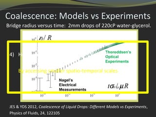
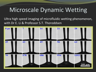
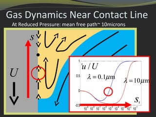
1) Computational techniques are essential for accurately simulating high-speed coating flows that conventional asymptotic models cannot capture. Accessing smaller spatio-temporal scales through computation and experiment is needed to identify the true physics. 2) Gas dynamics, particularly the mean free path of gas molecules, play a key role in phenomena like air entrainment in coating flows. At reduced pressures, the longer mean free path can delay air entrainment. 3) There is still debate around wetting because different models can describe experiments reasonably well using different parameter values. Fully resolving interfaces and accessing microscales may be needed to definitively identify the governing physics.

1. J.E. Sprittles (University of Oxford, U.K.)
Y.D. Shikhmurzaev (University of Birmingham, U.K.)
European Coating Symposium, Mons
September 2013

2. Coating Phenomena
Impact of a
solid on a liquid
Duez et al 07
Dip coating experiments
Courtesy of Terry Blake
Impact of a liquid on a solid
Xu et al 05

3. Questions
?
1) Why is there still so much debate about wetting?
2) Are computational techniques essential?
3) Are the gas’ dynamics important?
4) How can we identify the ‘true’ physics?

4. Coating Experiments
Advantages:
Flow is steady making
experimental analysis more
tractable.
Parameter space is easier to
map:
Speeds over 6 orders
Viscosities over 3 orders
appθ
clU Liquid
GasSolid
The
‘apparent angle’

5. Coating Results
Apparent angle measured at resolution of 20microns for
water-glycerol solutions with μ=1, 10, 100 mPas.
Increasing μ
cl
cl
U
Ca
µ
σ
=

6. You only observe the ‘apparent angle’. The actual one is fixed.
Free surface bends below the experiment’s resolution (20μm)
Interpretation A: Static Contact Angle
eθ
r
U
( )app rθ
The ‘actual angle’

7. Dynamics of angle cause change in apparent angle
Dynamic contact angle is a function of speed
Interpretation B: Dynamic Contact Angle
rU
dθ ( )app rθ

9. Slip Models
A: Equilibrium contact angle
B: Slip - typically Navier-slip
eθ
U ( )app rθ
ls
B: No-slip => No solution

10. Often, we have
Asymptotics for the Apparent Angle
( ) ( )
( )
( ) ( ) ( )
( ) ( ) ( ){ }
2 2
22 2 2
0
2 2
ln
sin cos sin
,
2sin 2 sin sin
( ) sin
app d
s
g
l
Lg g Ca
l
k K d
g k
k K k
K
k
θ
µ
µ
µ µ
µ
αθ θ
θ θ θ θ θ θ θ
θ
θ θ θ θ θ θ θ
θ θ θ
µ
µ
 = +  ÷
 
  Π − + + Π − −   =
  + Π − + + Π − −   
= −
=
∫
, 1sl
Ca
L
=
3 3
9 lnapp d
s
LCa
l
αθ θ  = +  ÷
 
( ) ( ) lnapp d
s
Lg g Ca
l
αθ θ  = +  ÷
 
1dθ =
In Cox 86, it was shown that in this case:
And for Voinov (76) has shown:

11. JES & YDS 2013, Finite Element Simulation of Dynamic Wetting Flows as an
Interface Formation Process, Journal of Computational Physics, 233, 34-65

12. Computational Domain
U Gas
Liquid
x1x10x10
8
x10
2
x10
4
Resolution:

13. Arbitrary Lagrangian Eulerian Mesh
Based on the ‘spine method’ of Scriven and co-workers
Microdrop simulation
with impact, spreading and rebound

15. Free Surface Profiles
With: 67 , 1nme slθ = =o

16. Computations vs Asymptotics
Ca=0.5
Ca=0.05
Ca=0.005
Solid line: Computations
Dashed line: Asymptotic (Cox’s) result

17. Limitations of Cox’s Formula
Chen, Rame & Garoff 95:
“Aspects of the unique hydrodynamics acting in the inner
region, not included in the model, project out and
become visible in the imaged region.”
0.1Ca = 0.5Ca =
( )r mµ
appθ
( )r mµ
appθ
2) Are computational techniques essential?
Yes!
To accurately capture high-speed coating flows.

18. Slip Model vs Experiments
Gas’ viscosity leads to air entrainment at a finite speed.
Decreasing viscosity ratio

20. Hydrodynamic Assist
U, cm/s
dθ
Blake et al 99
-1
(ms )U
appθ
appθ
Vary Flow
Rate
30dθ∆ ≈ o
U
Effect is not due to
free surface bending
(Wilson et al 06)

21. Physics of Dynamic Wetting
Make a dry solid wet.
Create a new/fresh liquid-solid interface.
Class of flows with forming interfaces.
Forming
interface
Formed interface
Liquid-solidLiquid-solid
interfaceinterface
SolidSolid

22. Relevance of the Young Equation
U
1 3 2cose e e eσ θ σ σ= − 1 3 2cos dσ θ σ σ= −
R
σ1e
σ3e - σ2e
Dynamic contact angle results from dynamic surface tensions.
The angle is now determined by the flow field.
Slip created by surface tension gradients (Marangoni effect)
θe θd
Static situation Dynamic wetting
σ1
σ3 - σ2
R

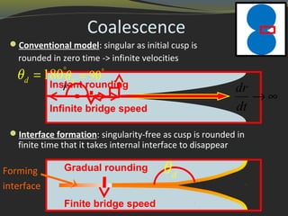
23. 2u 1
u 0, u u up
t
ν
ρ
∂
∇× = + ×∇ = − ∇ + ∇
∂
s s
1 1 1 2 2 2
1 3 2
v e v e 0
cos
s s
d
ρ ρ
σ θ σ σ
× + × =
= −
s
1
*
1
*
1
s 1 1
1
s 1 11
1 1
1 1|| ||
v 0
n [( u) ( u) ] n n
n [( u) ( u) ] (I nn) 0
(u v ) n
( v )
(1 4 ) 4 (v u )
s s
e
s ss
s e
s
f
f
t
p
t
µ σ
µ σ
ρ ρ
ρ
τ
ρ ρρ
ρ
τ
αβ σ β
∂
+ ×∇ =
∂
− + × ∇ + ∇ × = ∇×
× ∇ + ∇ × − + ∇ =
−
− × =
−∂
+ ∇ = −
∂
+ ∇ = −
In the bulk (Navier Stokes):
At contact lines:
On free surfaces:
Interface Formation Model
θd
e2
e1
n
n
f (r, t )=0
Interface Formation Modelling
( )*
2 || ||
s 2 2
2
s 2 22
2 2
2|| || || 2
2
1,2 1,2 1,2
1n [ u ( u) ] (I nn) u U
2
(u v ) n
( v )
1v (u U )
2
( )
s s
e
s ss
s e
s
s s
t
a b
µ σ β
ρ ρ
ρ
τ
ρ ρρ
ρ
τ
α σ
σ ρ ρ
×∇ + ∇ × − + ∇ = −
−
− × =
−∂
+ ∇ × = −
∂
= + = ∇
= −
Liquid-solid interface

24. Interface Formation vs Experiments
Apparent angle = Dynamic actual angle
1) Why is there still a debate about wetting?
Fundamentally different models describe experiments
(with reasonable parameter values).
+ Viscous bending

26. Influence of Gas Pressure
Splashing in Drop
Impact:
Xu, Zhang & Nagel 05
Air Entrainment Speed
in Dip Coating
Benkreira & Ikin 10

27. (Lack of) Influence of Inertia
 Bulk flow can’t be responsible for the effect.
Re = 0
Re = 100

28. Rarefied Gas Dynamics
Slip at solid-gas interface is due to finite mean free path.
Mean free path (hence Kn) depends on gas density.
λ 1Kn
L
λ
= =U
( )
u
Kn u U
y
∂
= −
∂

29. Gas Dynamics Near Contact Line
U
Atmospheric pressure: mean free path ~ 0.1 microns
/u U
s
s
0.1 mλ µ=

30. Gas Dynamics Near Contact Line
At Reduced Pressure: mean free path~ 10microns
/u U
s
U
s
0.1 mλ µ=
10 mλ µ=

31. Delayed Air Entrainment
Mean free paths (mfp) are:
Atmospheric pressure: mfp ~ 0.1 microns
Reduced pressure (10mbar): mfp ~ 10 microns
cCa
( )mfp mµ
3) Are the gas’ dynamics important?
Yes, its behaviour is key to air entrainment

33. Microdrop Impact
JES & YDS 2012, The Dynamics of Liquid Drops and their Interaction with
Solids of Varying Wettability, Physics of Fluids, 24, 082001.

34. Coalescence of Liquid Drops
Developed framework can be adapted for coalescence.
Thoroddsen’s Group:
Ultra high-speed imaging
Nagel’s Group:
Sub-optical electrical
measurements r
Thoroddsen et al 2005
dθ
Simulation
Experiment

35. Coalescence: Models vs Experiments
Bridge radius versus time: 2mm drops of 220cP water-glycerol.
Interface
formation
Conventional
Nagel’s
Electrical
Measurements
Thoroddsen’s
Optical
Experiments
/r R
/t Rσ µ
4) How can we identify the ‘true’ physics?
By accessing smaller spatio-temporal scales
JES & YDS 2012, Coalescence of Liquid Drops: Different Models vs Experiments,
Physics of Fluids, 24, 122105

36. Microscale Dynamic Wetting
Ultra high speed imaging of microfluidic wetting phenomenon,
with Dr E. Li & Professor S.T. Thoroddsen

37. Funding
Funding
This presentation is based on work supported by:

39. Computations vs Experiments
1.5, 10, 104 mPa sµ =Water-glycerol solutions of
& Asymptotics

40. Asymptotic Formula for Actual Angle in IFM
( ) ( )
( ) ( )
2 1 0
2
2
2 2 2 2 2
0
2 2 2 2
2 2
2
2 ( , )
cos cos
.
sin cos ( ) sin cos ( )
( , )
sin cos ( ) sin cos ( )
, ( ) sin
s s
e e d
e d s
e
d d d
d
d d d d
d
V u k
V V
V Sc Ca
K k K
u k
K k K
K
µ
µ
µ
µ
ρ ρ θ
θ θ
ρ
θ θ θ θ θ θ θ θ
θ
θ θ θ θ θ θ θ θ
θ θ θ θ θ
 + − =
+ +
=
− − −
=
− + −
= Π − = −
When there is no ‘hydrodynamic assist’, for small capillary
numbers the actual angle is dynamic:
Moffat 64

41. IFM vs Experiments
Shikhmurzaev 93
Shikhmurzaev 93 + Cox 86
& Asymptotics
Actual angle varies and free surface bends.

42. ‘Hydrodynamic Resist’
Smaller Capillaries
U
dθ
R
New effect: contact angle depends on capillary size
( m)R µ
Sobolev et al 01
dθ
1/3
U

43. Fibre Coating: Effect of Geometry
appθ
d
Simpkins & Kuck 03
appπ θ−
4mmd =
Uµ σ
2mmd =
U

44. Drop Spreading: Effect of Impact
Speed
1
0.18ms−
1
0.25ms−
)
U
appθ
-1
(ms )U
appθ
Bayer & Megaridis 06
30dθ∆ ≈ o

45. Coalescence
Conventional model: singular as initial cusp is
rounded in zero time -> infinite velocities
Interface formation: singularity-free as cusp is rounded in
finite time that it takes internal interface to disappear
Forming
interface
dθ
Instant rounding
Infinite bridge speed
90dθ °
=180dθ °
=
dr
dt
→ ∞
r
Gradual rounding
Finite bridge speed

46. Coalescence: Free surface profiles
Interface formation theory
Conventional theory
Water-
Glycerol
mixture of
230cP
Time: 0 < t < 0.1

47. 0.01 - 0.36
0.03 - 0.365
0.1 - 0.37
0.6 - 0.39
1 - 0.4
3 - 0.42
6 - 0.44
10 - 0.45
Wetting6 (1489) running 1166,2277 and 0.1microns –
saved previous t_info – running for current info

48. Microdrop Impact
25 micron water drop impacting at 5m/s on
left: wettable substrate right: nonwettable substrate