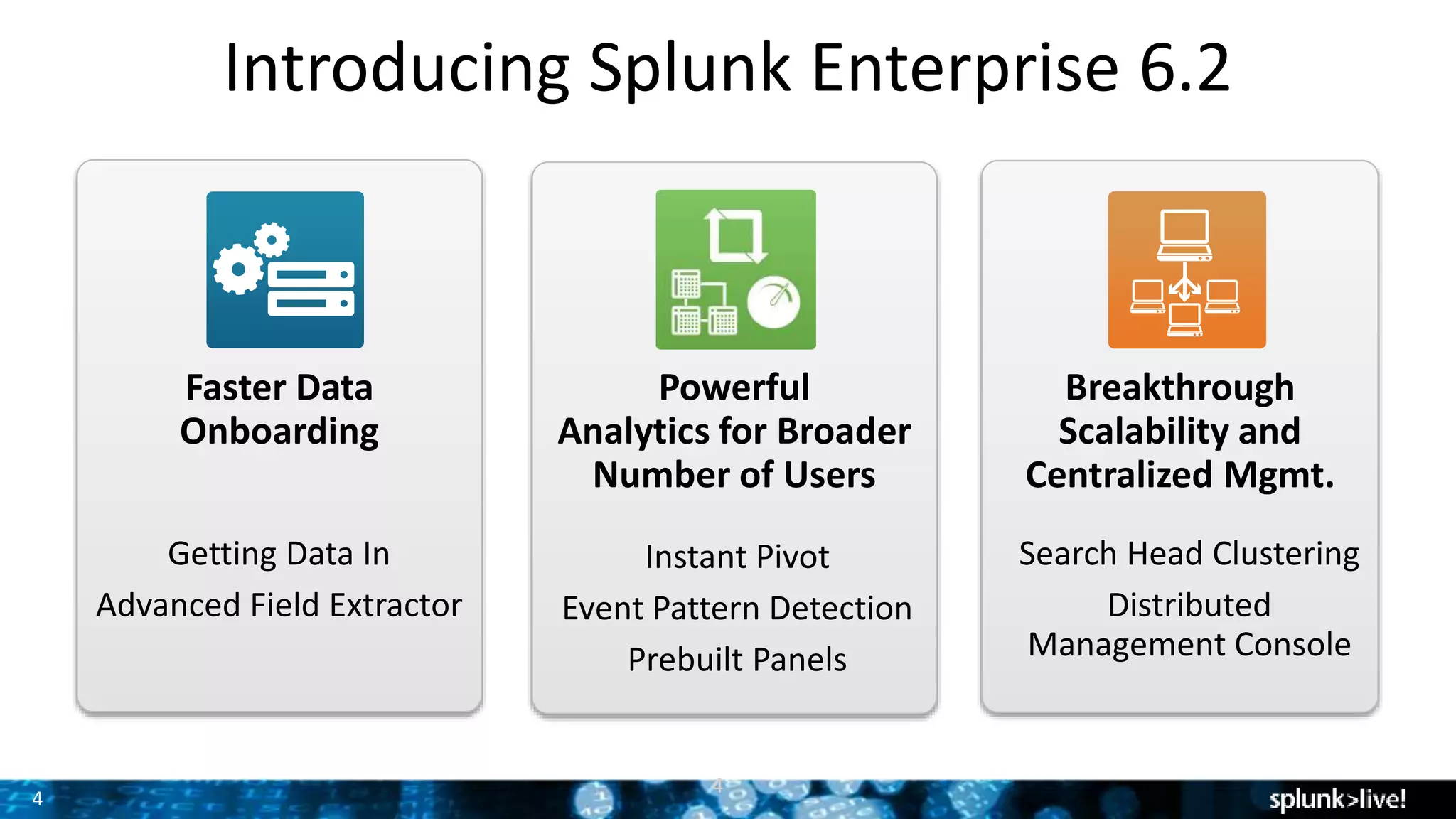
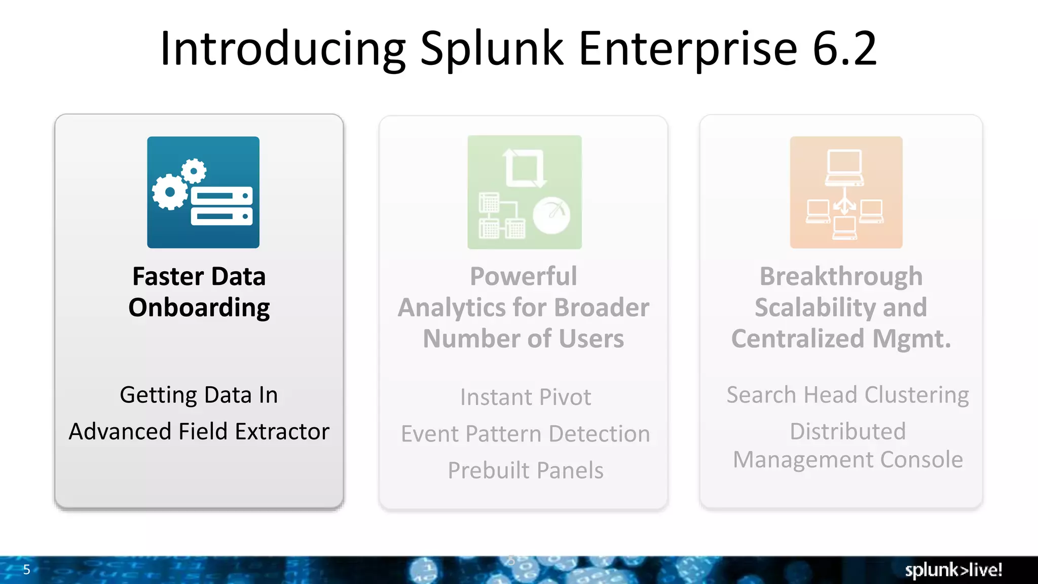
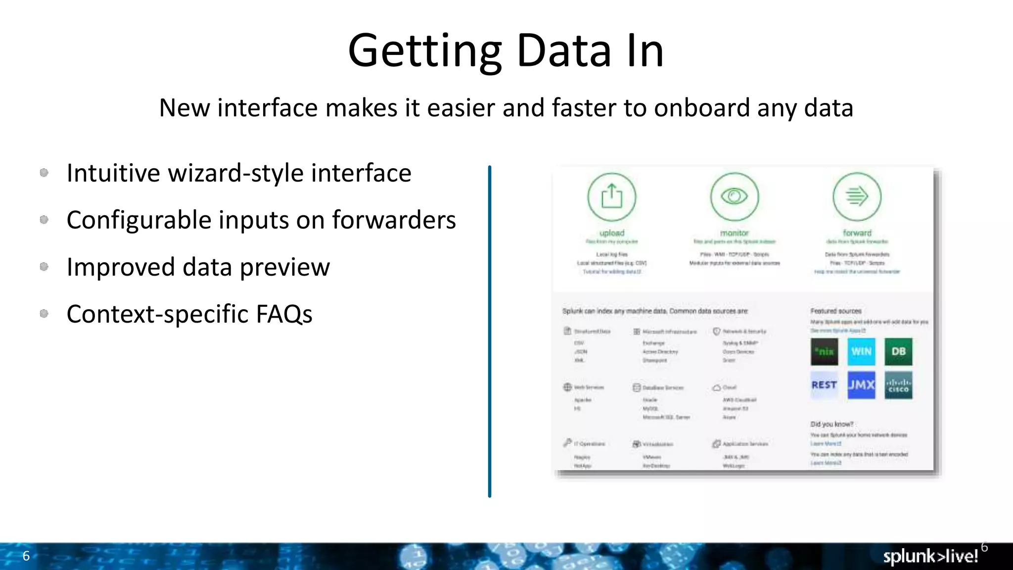
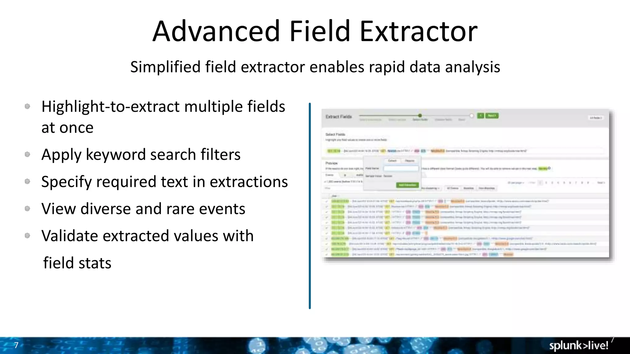
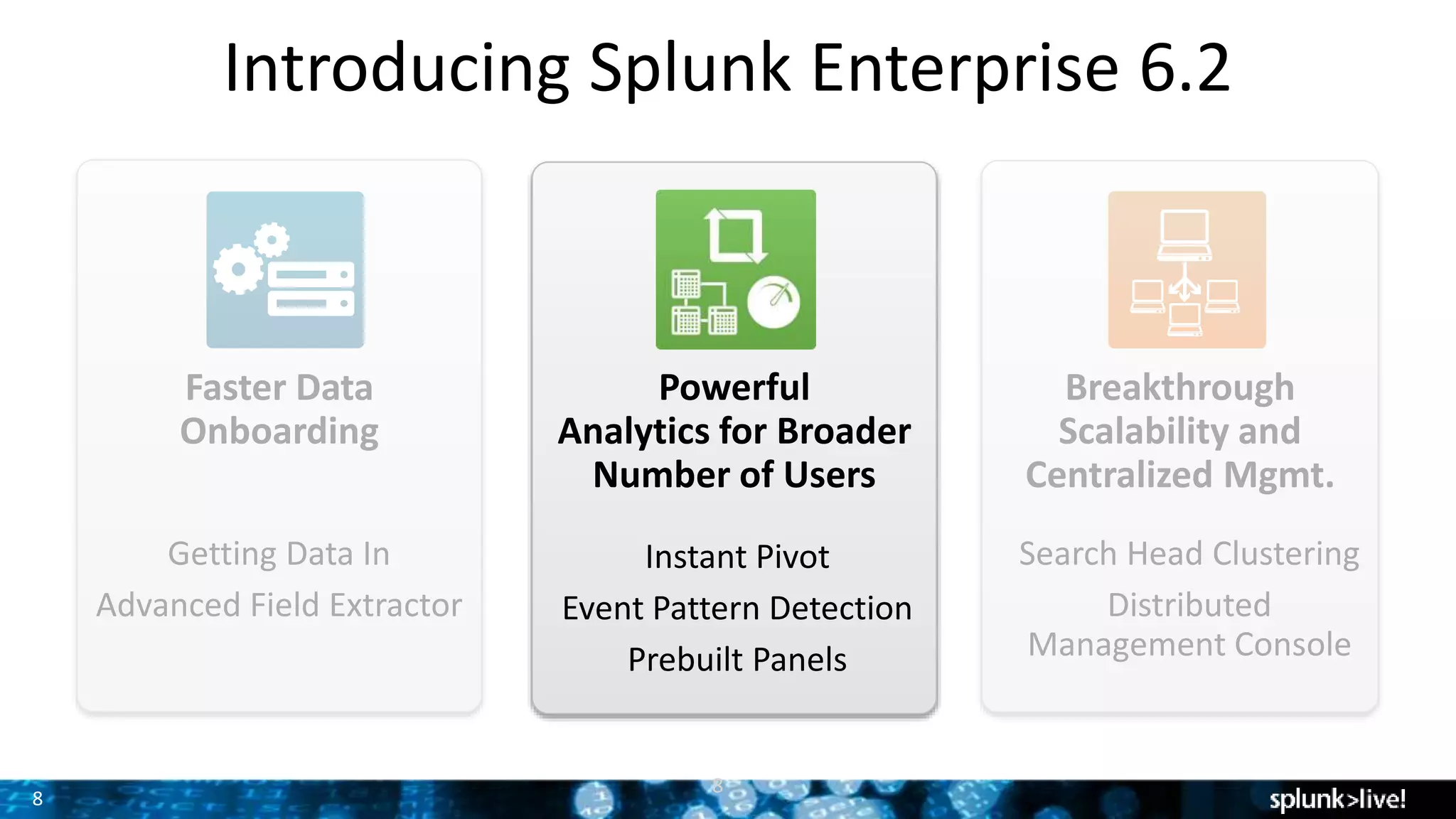
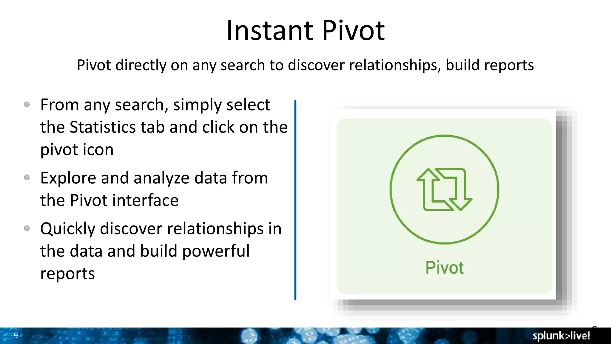
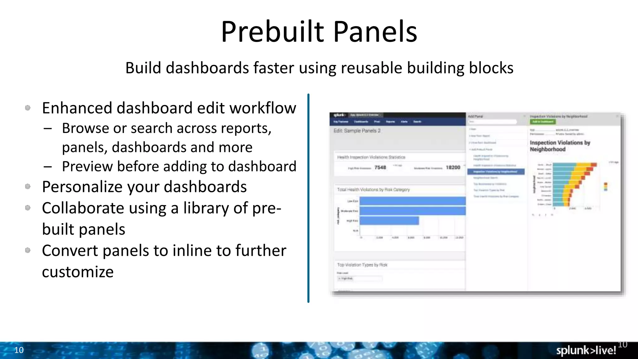
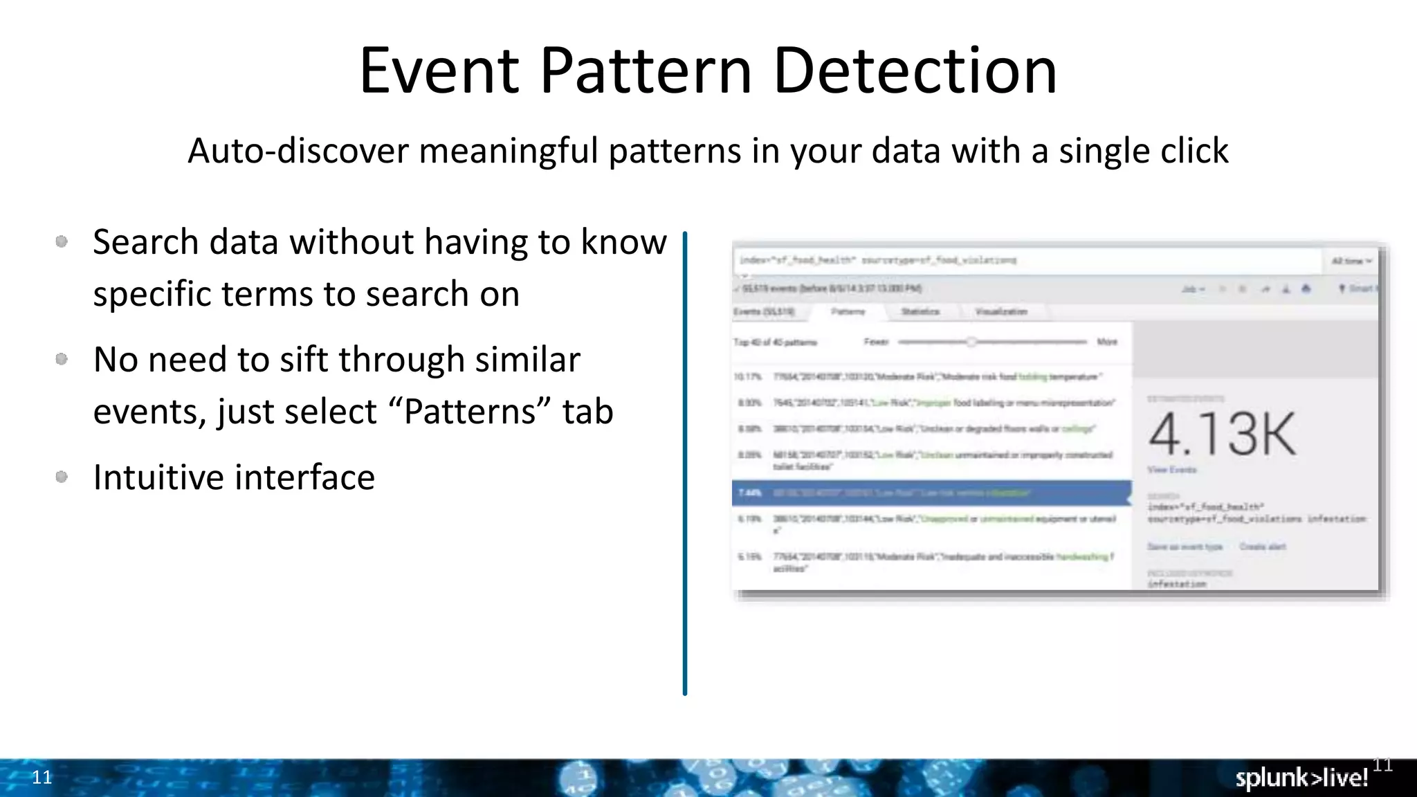
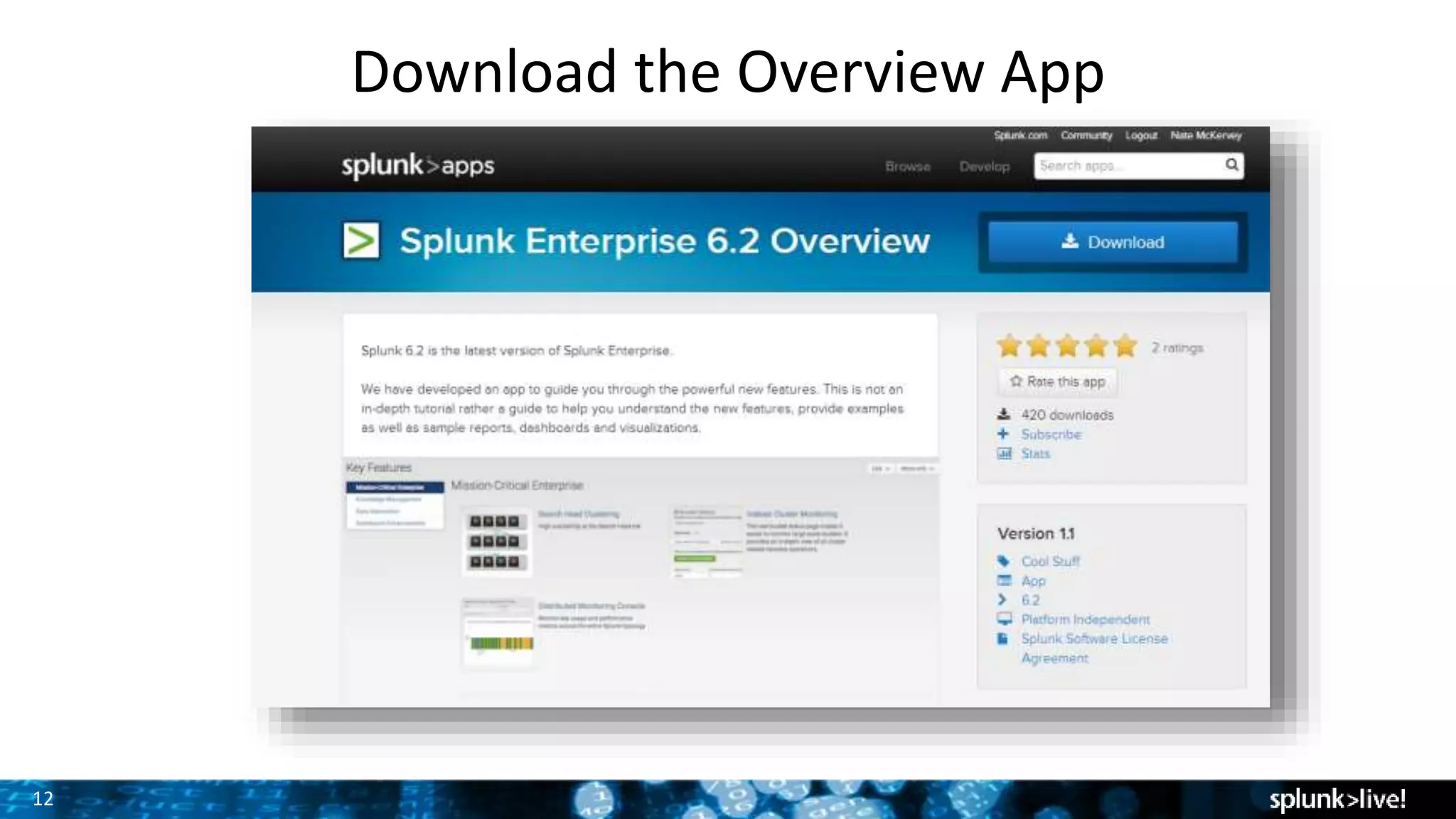
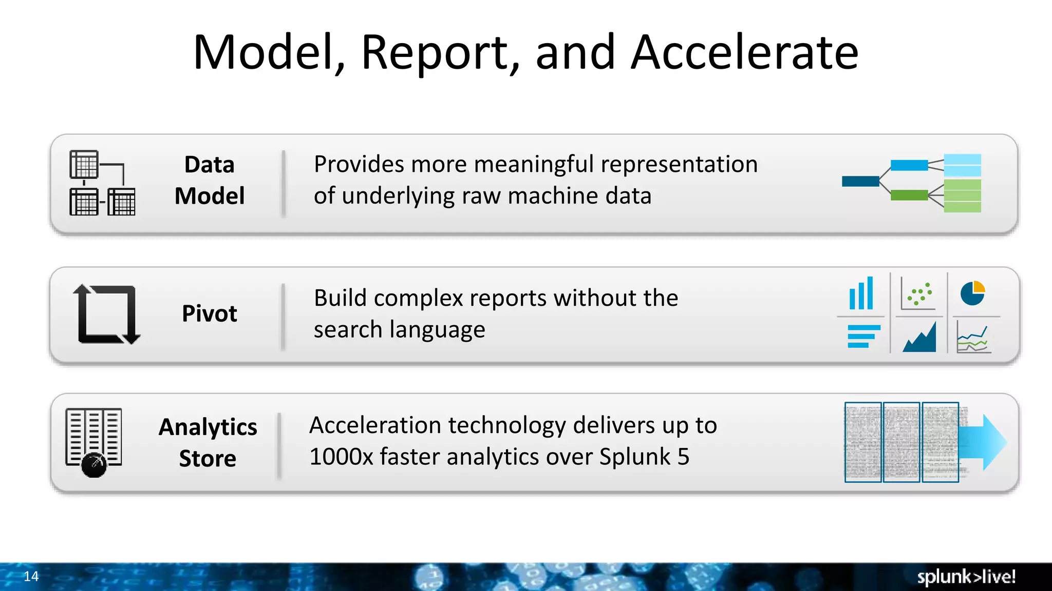
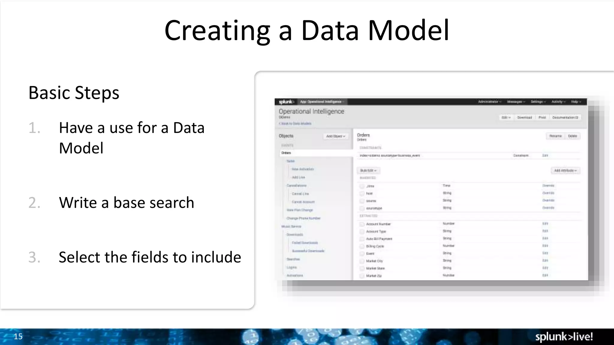
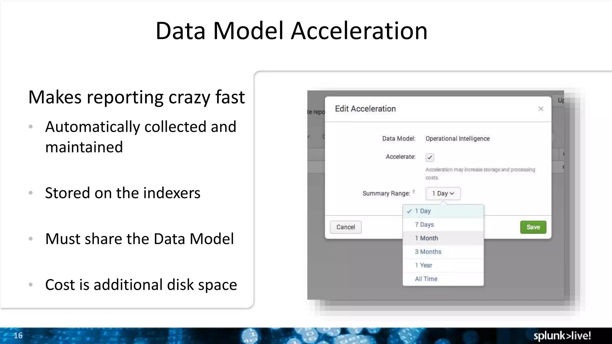
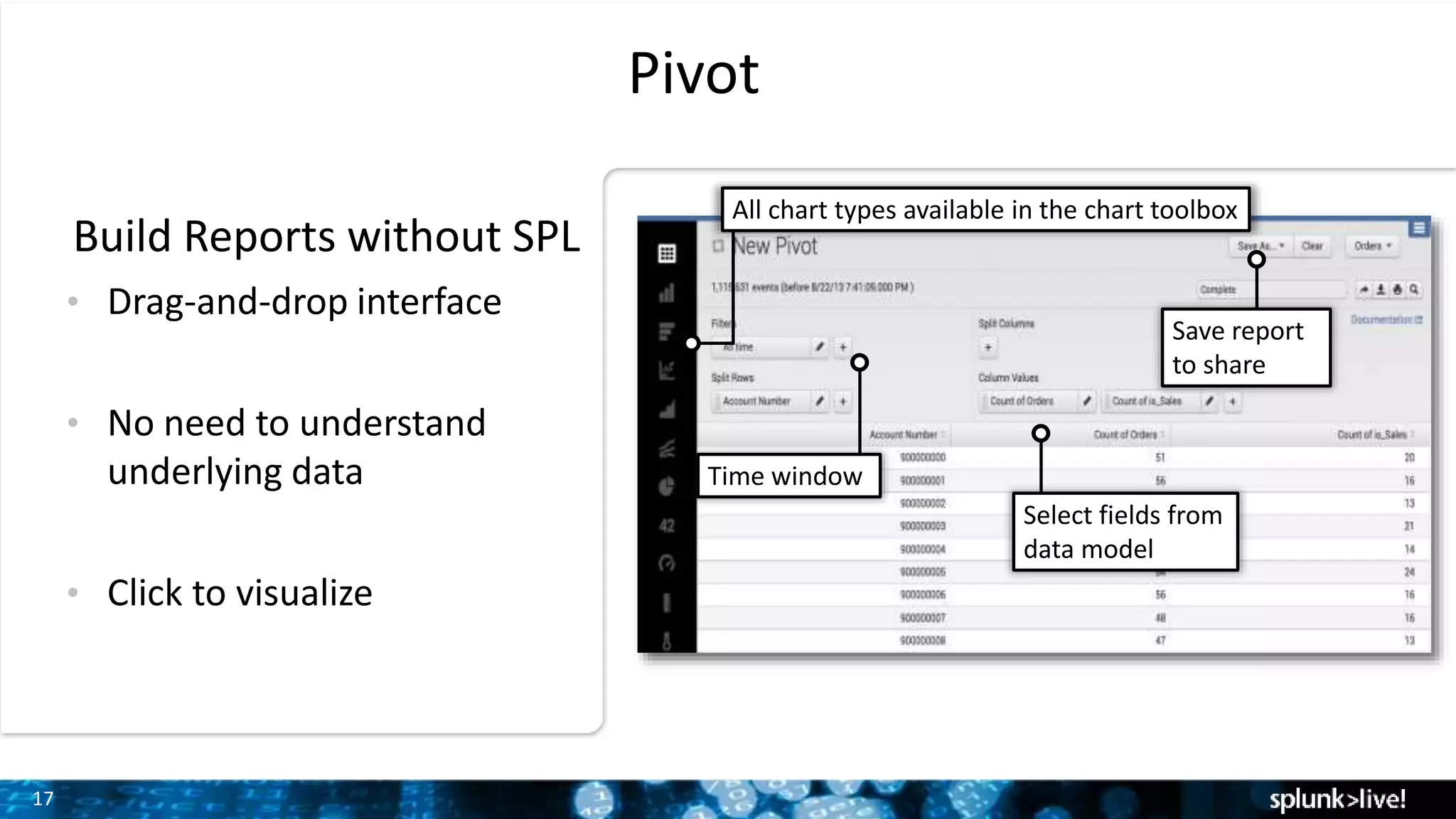
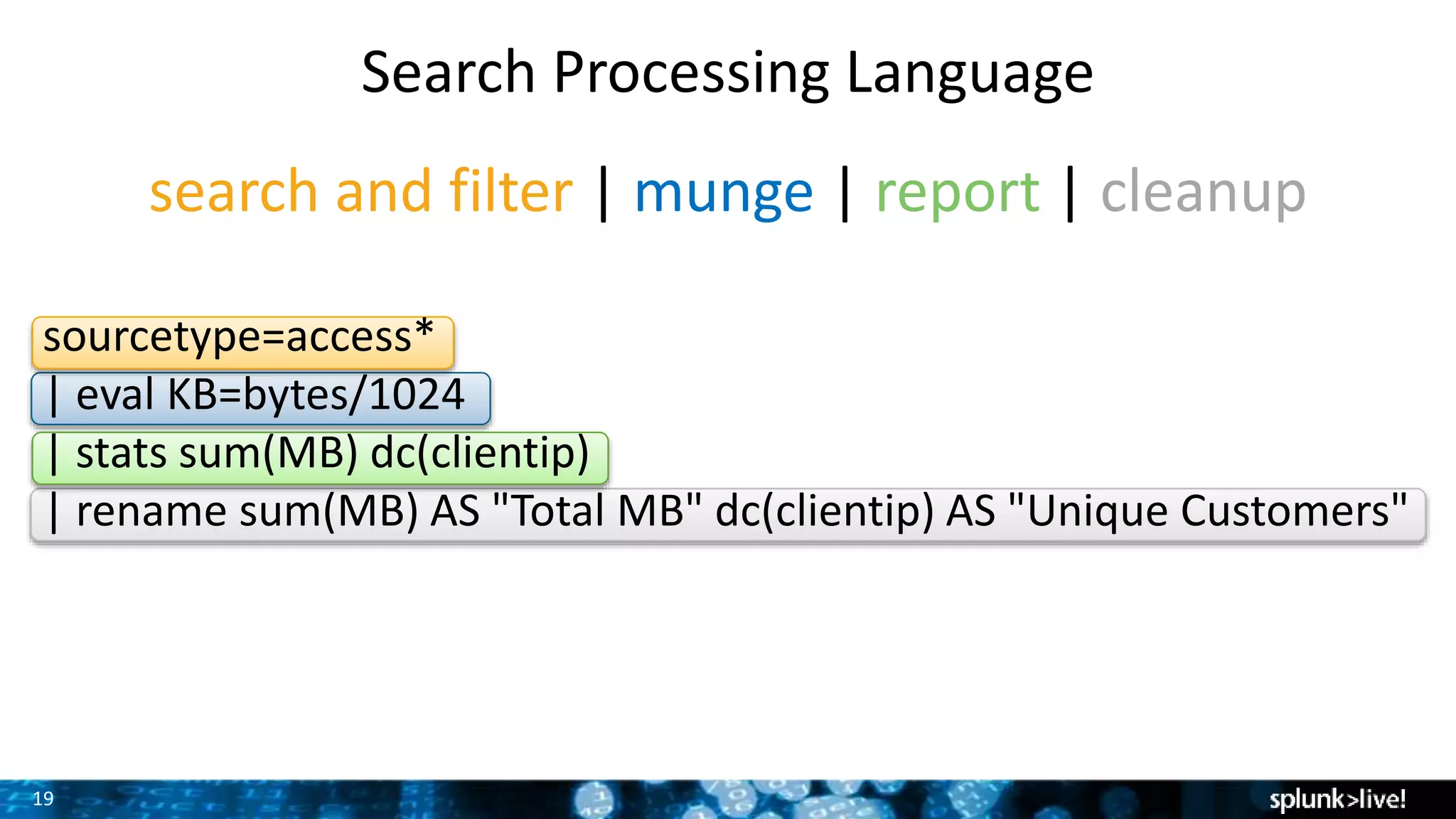
Besides seeing the newest features in Splunk Enterprise and learning the best practices for data models and pivot, we will show you how to use a handful of search commands that will solve most search needs. Learn these well and become a ninja.
2. 2
Safe Harbor Statement
During the course of this presentation, we may make forward looking statements regarding future events
or the expected performance of the company. We caution you that such statements reflect our current
expectations and estimates based on factors currently known to us and that actual events or results could
differ materially. For important factors that may cause actual results to differ from those contained in our
forward-looking statements, please review our filings with the SEC. The forward-looking statements
made in this presentation are being made as of the time and date of its live presentation. If reviewed
after its live presentation, this presentation may not contain current or accurate information. We do not
assume any obligation to update any forward looking statements we may make. In addition, any
information about our roadmap outlines our general product direction and is subject to change at any
time without notice. It is for informational purposes only and shall not be incorporated into any contract
or other commitment. Splunk undertakes no obligation either to develop the features or functionality
described orto includeany suchfeatureor functionalityina futurerelease.
3. 3
Agenda
What’s new in 6.2
– New features and capabilities
Data Models and Pivot
– Analyze data without using search commands
Harness the power of search
– The 5 search commands that can solve most problems
4. 4
Introducing Splunk Enterprise 6.2
4
Getting Data In
Advanced Field Extractor
Instant Pivot
Event Pattern Detection
Prebuilt Panels
Search Head Clustering
Distributed
Management Console
Powerful
Analytics for Broader
Number of Users
Faster Data
Onboarding
Breakthrough
Scalability and
Centralized Mgmt.
5. 5
Introducing Splunk Enterprise 6.2
5
Getting Data In
Advanced Field Extractor
Instant Pivot
Event Pattern Detection
Prebuilt Panels
Search Head Clustering
Distributed
Management Console
Powerful
Analytics for Broader
Number of Users
Faster Data
Onboarding
Breakthrough
Scalability and
Centralized Mgmt.
6. 6
Getting Data In
New interface makes it easier and faster to onboard any data
Intuitive wizard-style interface
Configurable inputs on forwarders
Improved data preview
Context-specific FAQs
6
7. 7
Advanced Field Extractor
Simplified field extractor enables rapid data analysis
Highlight-to-extract multiple fields
at once
Apply keyword search filters
Specify required text in extractions
View diverse and rare events
Validate extracted values with
field stats
7
8. 8
Introducing Splunk Enterprise 6.2
8
Getting Data In
Advanced Field Extractor
Instant Pivot
Event Pattern Detection
Prebuilt Panels
Search Head Clustering
Distributed
Management Console
Powerful
Analytics for Broader
Number of Users
Faster Data
Onboarding
Breakthrough
Scalability and
Centralized Mgmt.
9. 9
Instant Pivot
Pivot directly on any search to discover relationships, build reports
From any search, simply select
the Statistics tab and click on the
pivot icon
Explore and analyze data from
the Pivot interface
Quickly discover relationships in
the data and build powerful
reports
9
10. 10
Prebuilt Panels
Build dashboards faster using reusable building blocks
Enhanced dashboard edit workflow
– Browse or search across reports,
panels, dashboards and more
– Preview before adding to dashboard
Personalize your dashboards
Collaborate using a library of pre-
built panels
Convert panels to inline to further
customize
10
11. 11
Event Pattern Detection
Auto-discover meaningful patterns in your data with a single click
Search data without having to know
specific terms to search on
No need to sift through similar
events, just select “Patterns” tab
Intuitive interface
11
Screenshot or Image
suggestion
14. 14
Model, Report, and Accelerate
Build complex reports without the
search language
Provides more meaningful representation
of underlying raw machine data
Pivot
Data
Model
Acceleration technology delivers up to
1000x faster analytics over Splunk 5
Analytics
Store
15. 15
Creating a Data Model
Basic Steps
1. Have a use for a Data
Model
2. Write a base search
3. Select the fields to include
16. 16
Data Model Acceleration
• Automatically collected and
maintained
• Stored on the indexers
• Must share the Data Model
• Cost is additional disk space
Makes reporting crazy fast
17. 17
Pivot
• Drag-and-drop interface
• No need to understand
underlying data
• Click to visualize
Select fields from
data model
Time window
All chart types available in the chart toolbox
Save report
to share
Build Reports without SPL
19. 19
search and filter | munge | report | cleanup
Search Processing Language
sourcetype=access*
| eval KB=bytes/1024
| stats sum(MB) dc(clientip)
| rename sum(MB) AS "Total MB" dc(clientip) AS "Unique Customers"
20. 20
Five Commands that will Solve Most Data Questions
eval - Modify or Create New Fields and Values
stats - Calculate Statistics Based on Field Values
eventstats - Add Summary Statistics to Search Results
streamstats - Cumulative Statistics for Each Event
transaction - Group Related Events Spanning Time
24. 24
stats – Calculate Statistics Based on Field Values
Examples
• Calculate stats and rename
sourcetype=access*
| eval KB=bytes/1024
| stats sum(KB) AS “Total KB”
• Multiple statistics
sourcetype=access*
| eval KB=bytes/1024
| stats sum(KB) avg(KB)
• By another field
sourcetype=access*
| eval KB=bytes/1024
| stats sum(KB) avg(KB) by clientip
25. 25
stats – Calculate Statistics Based on Field Values
Examples
• Calculate stats and rename
sourcetype=access*
| eval KB=bytes/1024
| stats sum(KB) as “Total KB”
• Multiple statistics
sourcetype=access*
| eval KB=bytes/1024
| stats sum(KB) avg(KB)
• By another field
sourcetype=access*
| eval KB=bytes/1024
| stats sum(KB) avg(KB) by clientip
26. 26
stats – Calculate Statistics Based on Field Values
Examples
• Calculate statistics
sourcetype=access*
| eval KB=bytes/1024
| stats sum(KB) AS "Total KB”
• Multiple statistics
sourcetype=access*
| eval KB=bytes/1024
| stats avg(KB) sum(KB)
• By another field
sourcetype=access*
| eval KB=bytes/1024
| stats sum(KB) avg(KB) by clientip
27. 27
eventstats – Add Summary Statistics to Search Results
Examples
• Overlay Average
sourcetype=access*
| eventstats avg(bytes) AS avg_bytes
| timechart latest(avg_bytes) avg(bytes)
• Moving Average
sourcetype=access*
| eventstats avg(bytes) AS avg_bytes by date_hour
| timechart latest(avg_bytes) avg(bytes)
• By created field
sourcetype=access*
| eval http_response = if(status == 200, "OK", "Error”)
| eventstats avg(bytes) AS avg_bytes by http_response
| timechart latest(avg_bytes) avg(bytes) by http_response
28. 28
Examples
• Overlay Average
sourcetype=access*
| eventstats avg(bytes) AS avg_bytes
| timechart latest(avg_bytes) avg(bytes)
• Moving Average
sourcetype=access*
| eventstats avg(bytes) AS avg_bytes by date_hour
| timechart latest(avg_bytes) avg(bytes)
• By created field
sourcetype=access*
| eval http_response = if(status == 200, "OK", "Error”)
| eventstats avg(bytes) AS avg_bytes by http_response
| timechart latest(avg_bytes) avg(bytes) by http_response
eventstats – Add Summary Statistics to Search
Results
29. 29
eventstats – Add Summary Statistics to Search
Results
Examples
• Overlay Average
sourcetype=access*
| eventstats avg(bytes) AS avg_bytes
| timechart latest(avg_bytes) avg(bytes)
• Moving Average
sourcetype=access*
| eventstats avg(bytes) AS avg_bytes by date_hour
| timechart latest(avg_bytes) avg(bytes)
• By created field
sourcetype=access*
| eval http_response = if(status == 200, "OK", "Error”)
| eventstats avg(bytes) AS avg_bytes by http_response
| timechart latest(avg_bytes) avg(bytes) by http_response
30. 30
streamstats – Cumulative Statistics for Each Event
Examples
• Cumulative Sum
sourcetype=access*
| reverse
| streamstats sum(bytes) as bytes_total
| timechart max(bytes_total)
• Cumulative Sum by Field
sourcetype=access*
| reverse
| streamstats sum(bytes) as bytes_total by status
| timechart max(bytes_total) by status
• Moving Average
sourcetype=access*
| timechart avg(bytes) as avg_bytes
| streamstats avg(avg_bytes) AS moving_avg_bytes window=10
| timechart latest(moving_avg_bytes) latest(avg_bytes)
31. 31
streamstats – Cumulative Statistics for Each
Event
Examples
• Cumulative Sum
sourcetype=access*
| timechart sum(bytes) as bytes
| streamstats sum(bytes) as cumulative_bytes
| timechart max(cumulative_bytes)
• Cumulative Sum by Field
sourcetype=access*
| reverse
| streamstats sum(bytes) as bytes_total by status
| timechart max(bytes_total) by status
• Moving Average
sourcetype=access*
| timechart avg(bytes) as avg_bytes
| streamstats avg(avg_bytes) AS moving_avg_bytes window=10
| timechart latest(moving_avg_bytes) latest(avg_bytes)
32. 32
streamstats – Cumulative Statistics for Each
Event
Examples
• Cumulative Sum
sourcetype=access*
| timechart sum(bytes) as bytes
| streamstats sum(bytes) as cumulative_bytes
| timechart max(cumulative_bytes)
• Cumulative Sum by Field
sourcetype=access*
| reverse
| streamstats sum(bytes) as bytes_total by status
| timechart max(bytes_total) by status
• Moving Average
sourcetype=access*
| timechart avg(bytes) as avg_bytes
| streamstats avg(avg_bytes) AS moving_avg_bytes
window=10
| timechart latest(moving_avg_bytes) latest(avg_bytes)
33. 33
transaction – Group Related Events Spanning Time
Examples
• Group by Session ID
sourcetype=access*
| transaction JSESSIONID
• Calculate Session Durations
sourcetype=access*
| transaction JSESSIONID
| stats min(duration) max(duration) avg(duration)
• Stats is Better
sourcetype=access*
| stats min(_time) AS earliest max(_time) AS latest by JSESSIONID
| eval duration=latest-earliest
| stats min(duration) max(duration) avg(duration)
34. 34
transaction – Group Related Events Spanning
Time
Examples
• Group by Session ID
sourcetype=access*
| transaction JSESSIONID
• Calculate Session Durations
sourcetype=access*
| transaction JSESSIONID
| stats min(duration) max(duration) avg(duration)
• Stats is Better
sourcetype=access*
| stats min(_time) AS earliest max(_time) AS latest by JSESSIONID
| eval duration=latest-earliest
| stats min(duration) max(duration) avg(duration)
35. 35
transaction – Group Related Events Spanning
Time
Examples
• Group by Session ID
sourcetype=access*
| transaction JSESSIONID
• Calculate Session Durations
sourcetype=access*
| transaction JSESSIONID
| stats min(duration) max(duration) avg(duration)
• Stats is Better
sourcetype=access*
| stats min(_time) AS earliest max(_time) AS latest by JSESSIONID
| eval duration=latest-earliest
| stats min(duration) max(duration) avg(duration)
36. 36
Learn Them Well and Become a Ninja
eval - Modify or Create New Fields and Values
stats - Calculate Statistics Based on Field Values
eventstats - Add Summary Statistics to Search Results
streamstats - Cumulative Statistics for Each Event
transaction - Group Related Events Spanning Time
See many more examples and neat tricks at docs.splunk.com and answers.splunk.com
Here is what you need for this presentation:
Link to videos on box: <coming soon>
You should have the following installed:
6.2 Overview
OI Demo– Get it from the Technical Enablement Portal under SE tools –> Demos https://splunk--c.na2.visual.force.com/apex/LMS_TechnicalEnablementPortal
NOTE: Configure your role to search the oidemo index by default, otherwise you will have to type “index=oidemo” for the examples later on.
There is a lot to cover in this presentation! Try to go quickly and at a pretty high level. When you get through the presentation judge the audience’s interest and go deeper in whichever section. For example, if they want to know more about Pivot and Data Models then unhide those slides and walk through them, or if they want to go deeper on the search commands talk through the extra examples.
If running locally on 8000, these are the links to have ready in the background:
http://127.0.0.1:8000/en-US/app/oidemo/content_dashboard?form.track_name=Headlines&earliest=0&latest=
http://127.0.0.1:8000/en-US/app/oidemo/data_model_editor?model=%2FservicesNS%2Fnobody%2Foidemo%2Fdatamodel%2Fmodel%2FOIDemo
http://127.0.0.1:8000/en-US/app/oidemo/search
Splunk safe harbor statement.
Splunk Enterprise is the industry-leading platform for Operational Intelligence. Version 6.2 enables organizations to onboard, enrich and analyze machine data faster than ever before, scale to higher numbers of concurrent users and searches, and spend less time managing their large, distributed deployments.
Easier data onboarding and preparation
Getting Data In radically simplifies onboarding of any data source
Advanced Field Extractor enables better preparation of machine data for further analysis
More powerful analytics for everyone
Instant Pivot makes analytics easier by enabling anyone to Pivot directly on data, bypassing the Data Model step
Event Pattern Detection speeds analysis by identifying meaningful patterns in machine data
Prebuilt Panels enables faster dashboard creation by providing the ability to create and package re-usable dashboard building blocks
Simplified management at scale
Search Head Clustering enables horizontal scaling of the search head doubling the number of concurrent users and searches on the same hardware
Distributed Management Console delivers new management interface to centrally monitor distributed Splunk Enterprise deployments
In Splunk 6.2, we’ve completely remodeled the pages and workflows for adding data, and added new features like Forwarder Inputs a new Data Preview.
Consolidated Workflow:
We’ve made it much easier to find your way to the appropriate input configuration. Instead of selecting from a confusing list of sources, start with a simple choice of “upload, monitor, or forward” and you’ll find yourself in a simple wizard-style workflow of defining the appropriate parameters for the data you want to add.
Data Preview
The new Data Preview will make it easier for you to create the right sourcetype for your data. In the advanced section, you’ll be able to choose a charset from a list, and see how changes you make to your sourcetype are reflected in props.conf.
Forwarder Inputs
With Forwarder Inputs, you are able to push input configurations to Splunk instances configured as deployment clients. Simply select one or more forwarders and provide a group name, and you’ll be able to create data inputs on them in the same way you create inputs through the UI on your indexers.
With this enhancement, we’ve made it easier to extract fields from your data with the Advanced Field Extractor (AFX). A replacement of the existing field extraction utility, AFX enables you to easily capture multiple fields in a single extraction and specify required text to filter events for extraction (improving accuracy and efficiency). AFX also provides a number of methods for detecting false positives in order to help you validate your field extractions and improve the accuracy of your field
Splunk Enterprise is the industry-leading platform for Operational Intelligence. Version 6.2 enables organizations to onboard, enrich and analyze machine data faster than ever before, scale to higher numbers of concurrent users and searches, and spend less time managing their large, distributed deployments.
Easier data onboarding and preparation
Getting Data In radically simplifies onboarding of any data source
Advanced Field Extractor enables better preparation of machine data for further analysis
More powerful analytics for everyone
Instant Pivot makes analytics easier by enabling anyone to Pivot directly on data, bypassing the Data Model step
Event Pattern Detection speeds analysis by identifying meaningful patterns in machine data
Prebuilt Panels enables faster dashboard creation by providing the ability to create and package re-usable dashboard building blocks
Simplified management at scale
Search Head Clustering enables horizontal scaling of the search head doubling the number of concurrent users and searches on the same hardware
Distributed Management Console delivers new management interface to centrally monitor distributed Splunk Enterprise deployments
Instant Pivot enables you to open any query in the Pivot interface, without requiring the creation of a data model. This means that you have the flexibility to choose what interface to explore your data. This also creates another method to construct data models, starting with search.
When a user clicks on the Pivot icon, an ephemeral data model is created that collects user specified fields within Pivot as a single, flat object. The user can save their Pivot (additionally prompts user to save data model).
Users can choose to instantly Pivot on their data, modify fields, columns, etc in Pivot and then convert it back to a search if they need to use advanced search commands.
Instant Pivot allows users to interact with their data faster.
Panels allow users to build custom dashboards faster, leveraging pre-built dashboard panels packaged within apps. A user can select from pre-built reports and dashboards or create their own from the new Add Panel interface.
Event Pattern Detection reduces massive sets of data to its essence rather than sifting through all events. This can be used to identify common and rare events quickly or search your data without having to know specific terms to search on.
If you already understand the “cluster” command in Splunk then you know what this is capable of. A slide-bar allows you to set the threshold of similarity of the events so you can tune if you want the pattern to be more or less specific which will increase or reduce the number of patterns.
For more information, or to try out the features yourself. Check out the overview app which explains each of the features and includes code samples and examples where applicable.
This section should take ~10 minutes
Data Model – A data model is just like a map of the underlying data. It defines meaningful relationships in the data
Pivot – is an interface to analyze data without using the splunk search language
Analytics Store – is an option that can be applied to Data Models to make Pivot searches extremely fast. Think of it like our 3rd generation acceleration technology.
Let’s dig into each of these features
A data model is created by someone who has the domain knowledge of the underlying data. But first, why even create a data model?
Image is clickable
One great reason is so that others can leverage the domain knowledge without having to understand it. Think about it like this; if you are the expert on a particular data set, say web logs, you could build a data model that others can use and they won’t have to bother you if they want to analyze the data. For example, they won’t to ask you what a “purchase” looks like in the underlying data, they will be able to simply click on a “Purchase” object. Another bonus to data models is anyone will be able to analyze the data faster with Pivot. More on Pivot in a bit.
At a high level there are 3 steps to creating a Data Model.
Have a use– If you want to make it easier for users to analyze data themselves or you want to take advantage of the transparent acceleration technology of High Performance Analytics store (HPAS) then you have a good case to make a Data Model. Data Models are very cheap, they are simply a small JSON file and thus consume an insignificant amount of resources by themselves. Don’t be afraid to make multiple data models, even if they are very similar. For example, you might want a data model that is accelerated and another that is not of the same data since you cannot modify an accelerated data model without re-accelerating it.
Write a base search by adding an additional constraint via the “Add Object” dropdown.
Select the fields you want to include using “Add Attribute” dropdown.
Let’s take a look at a data model…
http://127.0.0.1:8000/en-US/app/oidemo/data_model_editor?model=%2FservicesNS%2Fnobody%2Foidemo%2Fdatamodel%2Fmodel%2FOIDemo
Show the OI Data Model
Data Models don’t have to be complex, even having just one root object is fine. Use “Root Event” whenever possible instead of “Root Search”. These searches can be optimized better.
Root search is for generating or streaming commands such as searches that begin with a |
Create a simple one one if you have time:
Root event: sourcetype=*
Child “Good responses” -> status<400
Child “Bad responses” -> status>=400
If you use instant pivot you can save the underlying data model that is automatically created.
<Briefly mention. It’s easy, its fast>
Automatically collected
Handles timing issues, backfill…
Automatically maintained
Uses acceleration window
Stored on the indexers
Peer to the buckets
Must share the Data Model
Acceleration can only be enabled if the Data Model is shared
Cost is additional disk space
Roughly 25% additional
New in 6.2, datamodels with multiple root events will be fully accelerated. In 6.1 only the first root event and children would be accelerated.
Why use Pivot?
The Pivot interface enables non-technical and technical users alike to quickly generate charts, visualizations and dashboards using simple drag and drop and without learning the Search Processing Language (SPL) and without having to have domain knowledge of the underlying data.
Queries using the Pivot interface are powered by underlying “data models” which we just spoke about that define the relationships in Machine Data.
<demo building a report using pivot, an example is provided in the hidden slides>
<This section should take ~15 minutes>Search is the most powerful part of Splunk.
The Splunk search language is very expressive and can perform a wide variety of tasks ranging from filtering to data, to munging, and reporting. The results can be used to answer questions, visualize results, or even send to a third party application in whatever format they require.
Although there are 135 documented search commands; however, most questions can be answered by using just a handful.
These are the five commands you should get very familiar with. If you know how to use these well, you will be able to solve most data questions that come your way. Let’s take a quick look at each of these.
sourcetype=access*
| eval KB=bytes/1024
| stats sum(KB) AS "Sum of KB"
sourcetype=access*
| stats values(useragent) avg(bytes) max(bytes) by clientip
sourcetype=access*
| stats values(useragent) avg(bytes) max(bytes) by clientip
Eventstats let’s you add statistics about the entire search results and makes the statistics available as fields on each event.
Let’s use eventstats to create a timechart of the average bytes on top of the overall average.
index=* sourcetype=access*
| eventstats avg(bytes) AS avg_bytes
| timechart latest(avg_bytes) avg(bytes)
We can turn this into a moving average simply by adding “by date_hour” to calculate the average per hour instead of the overall average.
index=* sourcetype=access*
| eventstats avg(bytes) AS avg_bytes by date_hour
| timechart latest(avg_bytes) avg(bytes)
To create a cumulative sum:
sourcetype=access*
| timechart sum(bytes) as bytes
| streamstats sum(bytes) as cumulative_bytes
| timechart max(cumulative_bytes)
sourcetype=access*
| reverse
| streamstats sum(bytes) as bytes_total by status
| timechart max(bytes_total) by status
sourcetype=access*
| timechart avg(bytes) as avg_bytes
| streamstats avg(avg_bytes) AS moving_avg_bytes window=10
| timechart latest(moving_avg_bytes) latest(avg_bytes)
Bonus: This could also be completed using the trendline command with the simple moving average (sma) parameter:
sourcetype=access*
| timechart avg(bytes) as avg_bytes
| trendline sma10(avg_bytes) as moving_average_bytes
| timechart latest(avg_bytes) latest(moving_average_bytes)
Double Bonus: Cumulative sum by period
sourcetype=access*
| timechart span=15m sum(bytes) as cumulative_bytes by status
| streamstats global=f sum(cumulative_bytes) as bytes_total
NOTE: Many transactions can be re-created using stats. Transaction is easy but stats is way more efficient and it’s a mapable command (more work will be distributed to the indexers).
sourcetype=access*
| stats min(_time) AS earliest max(_time) AS latest by JSESSIONID
| eval duration=latest-earliest
| stats min(duration) max(duration) avg(duration)
There is much more each of these commands can be used for. Check out answers.splunk.com and docs.splunk.com for many more examples.
<If you have time, feel free to show one of your favorite commands or a neat use case of a command. The cluster command is provided here as an example >
“There are over 135 splunk commands, the five you have just seen are incredibly powerful. Here is another to add to your arsenal.”
You can use the cluster command to learn more about your data and to find common and/or rare events in your data. For example, if you are investigating an IT problem and you don't know specifically what to look for, use the cluster command to find anomalies. In this case, anomalous events are those that aren't grouped into big clusters or clusters that contain few events. Or, if you are searching for errors, use the cluster command to see approximately how many different types of errors there are and what types of errors are common in your data.
Decrease the threshold of similarity and see the change in results
sourcetype=access* | cluster field=bc_uri showcount=t t=0.1| table cluster_count bc_uri _raw | sort -cluster_count